Weighted survival functional entropy and its properties

Ghadah Alomani; Mohamed Kayid

doi:10.1515/phys-2022-0234

Article Open Access

Weighted survival functional entropy and its properties

Ghadah Alomani and Mohamed Kayid

Published/Copyright: March 4, 2023

Published by

Become an author with De Gruyter Brill

Submit Manuscript Author Information Explore this Subject

From the journal Open Physics Volume 21 Issue 1

Abstract

The weighted generalized cumulative residual entropy is a recently defined dispersion measure. This article introduces a new uncertainty measure as a generalization of the weighted generalized cumulative residual entropy, called it the weighted fractional generalized cumulative residual entropy of a nonnegative absolutely continuous random variable, which equates to the weighted fractional Shannon entropy. Several stochastic analyses and connections of this new measure to some famous stochastic orders are presented. As an application, we demonstrate this measure in random minima. The new measure can be used to study the coherent and mixed systems, risk measure, and image processing.

Keywords: weighted fractional generalized cumulative residual entropy; generalized cumulative residual entropy; weighted mean residual lifetime; stochastic orders

1 Introduction and preliminaries

Shannon entropy is crucial in several areas of statistical mechanics and information theory. It is a well-known theory for uncertainty measures in the probabilistic framework that has attracted much attention in real applications, as seen in refs [1–4] among others. Boltzmann and Gibbs offered a widely used format of entropy in statistical mechanics, and Shannon provided it in information theory. If X is a discrete random variable with probability mass function P = ( p 1 , … , p n ) , then the fractional entropy is given by (see ref. [5])

(1) H α ( X ) = ∑ i = 1 n p i ( − log p i ) α , 0 ≤ α ≤ 1 .

It is obvious that (1) is a nonnegative criterion. Moreover, it has the properties of concavity and nonadditivity. In the particular case for α = 1 , it reduces to Shannon entropy [6]. From (1), it is clear that the fractional entropy is a function of p i , and the values of the random variables do not matter. For this reason, and to obtain a better uncertainty analysis, the probabilities and qualitative aspects of the possibilities in many domains must be considered under different circumstances (see, e.g., [7]). For this purpose, the notion of weighted fractional entropy is determined by

(2) H α w ( X ) = ∑ i = 1 n w i p i ( − log p i ) α , 0 ≤ α ≤ 1 .

It is clear that (2) reduces to (1) for w i = 1 , i = 1 , … , n , and equals to the weighted entropy when α = 1 .

The cumulative residual entropy (CRE) was introduced by ref. [8], and the fractional CRE was presented by ref. [9]. Recently, the fractional generalized cumulative residual entropy (FGCRE) of X as an extension of CRE was developed in ref. [10] as follows:

(3) E α ( X ) = q ( α ) ∫ 0 ∞ S ( x ) [ Θ ( x ) ] α d x ,

where q ( α ) = 1 Γ ( α + 1 ) , α ≥ 0 , such that

(4) Θ ( x ) = − log S ( x ) = ∫ 0 x λ ( u ) d u , x > 0 ,

and λ ( u ) = f ( u ) / S ( u ) , u > 0 , denotes the hazard rate function. Other properties of the quoted measure are found in refs [9,11,12] and the references therein. As suggested by ref. [10], if α = n ∈ N , then E n ( X ) reduces to the generalized cumulative residual entropy introduced in ref. [13]. Several properties and applications of some uncertainty measures have been considered in the literature. For example, some other properties of the CRE were studied in ref. [14] and were applied to coherent and mixed systems. In addition, in ref. [15], the generalized CRE was considered as a risk measure and was compared to the standard deviation and the right-tail risk measure. Recently, in ref. [16], the cumulative residual Tsallis entropy was used as an alternative measure of uncertainty in blind assessment of the image quality. In this article, we aim to present a new measure of uncertainty determined by the weighted FGCRE. It is worth noting that the new measure is particularly important in the context of the proportional hazard rate model. Based on the mentioned references, the new measure can be used to study coherent and mixed systems, risk measurement, and image processing.

The remainder of this article is thus structured as follows. Section 2 introduces a new measure of uncertainty through the weighted FGCRE. We then provide some expressions for the weighted fractional generalized cumulative residual entropy (WFGCRE), one of which is associated with the weighted mean residual life (WMRL) function. In Section 3, we study the stochastic ordering properties of the WFGCRE and then provide some bounds for it. In Section 4, we conclude the article with some remarks and directions for the future work.

Before discussing our main results, we should recall some stochastic orders and classes of life distributions that we will use in the sequel. For more details, we refer the reader to ref. [17]. For this purpose, throughout this article, we denote the collection of absolutely continuous nonnegative random variables containing the support ( 0 , ∞ ) by R + = { X ; X ≥ 0 } . Moreover, we assume that α ∈ D + , where D + = [ 0 , ∞ ) .

Definition 1.1

Let X 1 ∈ R + have cumulative distribution function (CDF) F 1 ( x ) , probability density function (pdf) f 1 ( x ) , survival function S 1 ( x ) = 1 − F 1 ( x ) , hazard rate function λ 1 ( x ) , and mean residual life (MRL) function m 1 ( x ) = 1 S 1 ( t ) ∫ t ∞ S 1 ( x ) d x . Similarly, let X 2 ∈ R + have CDF F 2 ( x ) , PDF f 2 ( x ) , survival function S 2 ( x ) = 1 − F 2 ( x ) , hazard rate function λ 2 ( x ) , and MRL function m 2 ( x ) = 1 S 2 ( t ) ∫ t ∞ S 2 ( x ) d x . Then:

X 1 has the (increasing) decreasing MRL (IMRL (DMRL)) property if m 1 ( x ) is increasing (decreasing) in x > 0 ;
X 1 has the (increasing) decreasing failure rate (IFR(DFR)) property if λ 1 ( x ) is increasing (decreasing) in x > 0 ;
X 1 is smaller than X 2 in the usual stochastic order (denoted by X 1 ≤ s t X 2 ) if S 1 ( x ) ≤ S 2 ( x ) , ∀ x > 0 .
X 1 is smaller than X 2 in the hazard rate order (denoted by X 1 ≤ h r X 2 ) if S 1 ( x ) S 2 ( y ) ≥ S 2 ( x ) S 1 ( y ) for all x ≤ y .
X 1 is smaller than X 2 in the likelihood ratio order (denoted by X 1 ≤ l r X 2 ) if f 1 ( x ) f 2 ( y ) ≥ f 1 ( y ) f 2 ( x ) for all x ≤ y , with x , y > 0 .
X 1 is smaller than X 2 in the MRL order (denoted by X 1 ≤ m r l X 2 ) if m 1 ( x ) ≤ m 2 ( x ) for all x ≥ 0 .
X 1 is smaller than X 2 in the increasing convex order (denoted by X 1 ≤ i c x X 2 ) if E [ Φ ( X 1 ) ] ≤ E [ Φ ( X 2 ) ] for all increasing convex functions Φ ( ⋅ ) such that the expectations exist.

2 New uncertainty measure

In this section, we propose WFGCRE and investigate its manifold properties. For this purpose, let X ∈ R + with CDF F and PDF f . Moreover, we consider an increasing nonnegative differentiable function Ψ ( x ) such that Ψ ′ ( x ) = ϕ ( x ) ≥ 0 . Then the WFGCRE of X is represented by

(5) E α Ψ ( X ) = q ( α ) ∫ 0 ∞ ϕ ( x ) S ( x ) [ Θ ( x ) ] α d x ,

for all α ∈ D + , provided the right-hand side integral is finite. It is worth noting that our results are the generality of the weighted generalized cumulative residual entropy (WGCRE) from [18]. It is obvious that (5) is nonnegative and equal to zero when X has a degenerate distribution function. In the particular case α = 1 , we have the weighted CRE as follows:

(6) E w ( X ) = ∫ 0 ∞ ϕ ( x ) S ( x ) Θ ( x ) d x ,

Here, we obtain an expression for the WFGCRE that is a generalization (24) in ref. [18] for the WGCRE. For this purpose, we define the random variable X α + 1 with the PDF as follows:

(7) f α + 1 ( x ) = 1 Γ ( α + 1 ) [ Θ ( x ) ] α f ( x ) , x ≥ 0 ,

for all α ∈ D + . The definition of Θ ( x ) is defined in (4). If we denote the survival function of X α + 1 by S α + 1 ( x ) , it holds that S α + 1 ( x ) = K α + 1 ( S ( x ) ) , x ≥ 0 , where

K α + 1 ( t ) = q ( α ) ∫ 0 t ( − log u ) α d u , 0 < t < 1

is an increasing function of t for all α ∈ D + .

Proposition 2.1

Let X ∈ R + . Then,

(8) E α Ψ ( X ) = E [ Ψ ( X α + 1 ) ] − E [ Ψ ( X α ) ] ,

for all α ∈ D + .

Proof

From (5), we have

E α Ψ ( X ) = q ( α ) { Ψ ( α ) − α Ψ ( α − 1 ) } = ∫ 0 ∞ Ψ ( x ) f α + 1 ( x ) d x − α Γ ( α ) Γ ( α + 1 ) ∫ 0 ∞ Ψ ( x ) f α ( x ) d x = E [ Ψ ( X α + 1 ) ] − E [ Ψ ( X α ) ] ,

where ϒ ( α ) = ∫ 0 ∞ Ψ ( x ) [ Θ ( x ) ] α f ( x ) d x , and the first equality is acquired using integrating by parts, while the last equality is received by remembering (7) and utilizing the identity Γ ( α + 1 ) = α Γ ( α ) (Table 1).

Table 1

WFGCRE for some specific parametric distributions

Distribution	S ( x )	Ψ ( x ) = x	Ψ ( x ) = x 2
Uniform ( 0 , b )	1 − x b , 0 ≤ x ≤ b , b > 0	b 2 α + 1	2 b 1 2 α + 1 − 1 3 α + 1
Weibull ( 1 , k )	e − x k , x > 0 , k > 0	Γ α + 1 k k Γ ( α + 1 )	2 Γ ( α + 2 k ) k Γ ( α + 1 )
Beta ( 1 , b )	( 1 − x ) b , 0 ≤ x ≤ 1 , b > 1	b α ( b − 1 ) α + 1	2 b α 1 ( b + 1 ) α + 1 − 1 ( b + 2 ) α + 1

From Proposition 2.1, we note that E α Ψ ( X ) is the location between the functions

S Ψ , α + 1 ( x ) = P ( Ψ ( X α + 1 ) > x ) = K α + 1 ( S ( Ψ − 1 ( x ) ) ) ,

and

S Ψ , α ( x ) = P ( Ψ ( X α ) > x ) = K α ( S ( Ψ − 1 ( x ) ) ) ,

for all α ∈ D + . In certain, E 0 Ψ ( X ) = E ( Ψ ( X ) ) is the location under S Ψ , 1 ( x ) = P ( Ψ ( X 1 ) > x ) . Figure 1 displays these locations for a standard exponential distribution and different values of α for Ψ ( x ) = x 2 (top panel) and Ψ ( x ) = x (bottom panel). Also notice from (5) that the WFGCRE can be written as follows:

(9) E α Ψ ( X ) = E ϕ ( X α + 1 ) λ ( X α + 1 ) ,

for all α ∈ D + . The following theorem gives a sufficient condition for the WFGCRE to be finite.

$Figure 1 S x 2 , α ( x ) = P ( X α 2 > x ) {S}_{{x}^{2},\alpha }\left(x)=P\left({X}_{\alpha }^{2}\gt x) (top panel) and S x , α ( x ) = P ( X α > x ) {S}_{\sqrt{x},\alpha }\left(x)=P\left({\sqrt{X}}_{\alpha }\gt x) (bottom panel) for an exponential distribution for α = 1 , 1.5 , 2 , 2.5 , 3 , 3.5 \alpha =1,1.5,2,2.5,3,3.5 .$

Figure 1

S x 2 , α ( x ) = P ( X α 2 > x ) (top panel) and S x , α ( x ) = P ( X α > x ) (bottom panel) for an exponential distribution for α = 1 , 1.5 , 2 , 2.5 , 3 , 3.5 .

Theorem 2.1

Let X ∈ R + . If 0 ≤ ϕ ( x ) ≤ 1 , then

if E ( Ψ ( X p ) ) < ∞ for some p > 1 / α , then E α Ψ ( X ) < ∞ , ∀ 0 < α ≤ 1 .
if E ( Ψ ( X p ) ) < ∞ for some p > α , then E α Ψ ( X ) < ∞ , ∀ α ∈ [ 1 , ∞ ) .

Proof

(i) From relation (13) of ref. [12] for all α , β ∈ [ 0 , 1 ] , one can obtain

(10) x ( − log x ) α ≤ α e − 1 1 − β α x β , 0 ≤ x ≤ 1 ,

and hence, by taking β = α for α ∈ [ 0 , 1 ] , we obtain

x ( − log x ) α ≤ α e − 1 1 − α α x α , 0 ≤ x ≤ 1 .

From this and noting that 0 ≤ ϕ ( x ) ≤ 1 , we obtain

(11) E α Ψ ( X ) ≤ c ( α ) ∫ 0 ∞ ϕ ( x ) S α ( x ) d x = c ( α ) ∫ 0 1 ϕ α ( x ) d x + ∫ 1 ∞ ϕ α ( x ) d x ≤ c ( α ) 1 + ∫ 1 ∞ S α ( x ) d x ≤ c ( α ) 1 + ∫ 1 ∞ E ( X p ) x p α d x = c ( α ) 1 + [ E ( X p ) ] α ∫ 1 ∞ 1 x α p d x ,

where h α ( x ) = ϕ ( x ) S α ( x ) and c ( α ) = q ( α ) α e − 1 1 − α α . The third inequality in (11) is conveyed using Markov’s inequality, while the final integral is finite if p ∈ 1 α , ∞ , and this ends the proof. In the case where α ∈ [ 1 , ∞ ) , we set β = 1 / α .□

An alternative indication for the WFGCRE of X is supplied in the forthcoming theorem. It is represented regarding the cumulative hazard function of X provided by (4).

Theorem 2.2

Let X ∈ R + with finite WFGCRE function E α Ψ ( X ) < + ∞ for all α ∈ D + . We have,

(12) E α Ψ ( X ) = E [ Ω Ψ , α ( 2 ) ( X ) ] ,

such that

(13) Ω Ψ , α ( 2 ) ( x ) = q ( α ) ∫ 0 x ϕ ( t ) Θ α ( t ) d t , x ≥ 0 .

Proof

From (5) and Fubini’s theorem, we obtain

E α Ψ ( X ) = q ( α ) ∫ 0 ∞ ϕ ( t ) ∫ t ∞ f ( x ) d x Θ α ( t ) d t = q ( α ) ∫ 0 ∞ f ( x ) ∫ 0 x ϕ ( t ) Θ α ( t ) d t d x ,

which immediately follows (12) by using (13).□

This immediately allows us to obtain the following theorem.

Theorem 2.3

Let X ∈ R + with mean μ = E ( X ) < ∞ . If Ψ ( x ) is an increasing convex function, then

E α Ψ ( X ) ≥ Ω Ψ , α ( 2 ) ( μ ) ,

for all α ∈ D + .

Proof

Based on the assumption, Ω Ψ , α ( 2 ) ( x ) in (13) is an increasing convex function of x . This implies the result.□

Another useful application of Theorem 2.2 is given in the next theorem.

Theorem 2.4

Let X , Y ∈ R + . If Ψ ( x ) is an increasing convex function and X ≤ i c x Y , then

Ω Ψ , α ( 2 ) ( X ) ≤ i c x Ω Ψ , α ( 2 ) ( Y ) , α ∈ D +

where the function Ω Ψ , α ( 2 ) ( ⋅ ) is defined in (13). Specifically, X ≤ i c x Y yields

E α Ψ ( X ) ≤ E α Ψ ( Y ) .

Proof

Since the function Ω Ψ , α ( 2 ) ( ⋅ ) is an increasing convex function for all α ∈ D + , it follows (see Theorem 4.A.8 of ref. [17]) that Ω Ψ , α ( 2 ) ( X ) ≤ i c x Ω Ψ , α ( 2 ) ( Y ) , α ∈ D + . Now, using relation 4.A.2 of ref. [17], we derive E α Ψ ( X ) ≤ E α Ψ ( Y ) .□

As another example of the use of Theorem 2.2, when Ψ ( x ) is an increasing convex function, it can be seen that the function Ω Ψ , α ( 2 ) ( ⋅ ) is an increasing convex function such that Ω Ψ , α ( 2 ) ( 0 ) = 0 . So if X ≤ h r Y , we have

(14) E α Ψ ( X ) E ( X ) ≤ E α Ψ ( Y ) E ( Y ) ,

for all α ∈ D + . This connection is directly acquired from Theorem 2.2 and appealing to [17] (see page 24). We note that Eq. (14) guides us to specify the normalized WFGCRE by

(15) Nℰ α Ψ ( X ) = E α Ψ ( X ) E ( X ) .

Under the condition X ≤ h r Y , the outcome of Eq. (14) can be declared as Nℰ α Ψ ( X ) ≤ Nℰ α Ψ ( Y ) for α ∈ D + . We now recall the WMRL function defined by m ψ ( t ) = E [ ψ ( X ) − ψ ( t ) ∣ X > t ] , obtained by the next formula:

(16) m ψ ( t ) = 1 F ¯ ( t ) ∫ t ∞ ϕ ( x ) F ¯ ( x ) d x

for all t ≥ 0 such that F ¯ ( t ) > 0 ; see [18]. It is evident that m ψ ( 0 ) = E [ ψ ( X ) ] . In the next theorem, we supply another term for the WFGCRE regarding the expectation of the WMRL function, described in (16), evaluated at X α .

Theorem 2.5

For X ∈ R + , one has

(17) E α Ψ ( X ) = E ( m ψ ( X α ) ) .

Proof

For all α ∈ D + , we have

∫ 0 t Θ α − 1 ( x ) Γ ( α ) λ ( x ) d x = Θ α ( t ) Γ ( α + 1 ) , t ≥ 0 ,

where the last equality is obtained by noting that Γ ( α + 1 ) = α Γ ( α ) . From this, Eq. (5) and using Fubini’s theorem, we have

(18) E α Ψ ( X ) = ∫ 0 ∞ ϕ ( t ) Θ α ( t ) Γ ( α + 1 ) S ( t ) d t = ∫ 0 ∞ ∫ 0 t Θ α − 1 ( x ) Γ ( α ) λ ( x ) ϕ ( t ) S ( t ) d x d t , = ∫ 0 ∞ Θ α − 1 ( x ) Γ ( α ) λ ( x ) ∫ x ∞ ϕ ( t ) S ( t ) d t d x = ∫ 0 ∞ m ψ ( x ) Θ α − 1 ( x ) Γ ( α ) f ( x ) d x .

The last equality in (18) is concluded from (16). So, Eq. (17) now is obtained from (7).□

The subsequent example applies relation (17) for the minimum of a random sample, which may be considered as the lifetime of a series system.

Example 2.1

Let X 1 : m = min { X 1 , … , X m } , where X 1 , … , X m are absolutely continuous nonnegative random variables having CDF F ( x ) . If we assume the survival function of X 1 : m by F ¯ 1 : m ( x ) = P ( X 1 : m > x ) = [ F ¯ ( x ) ] m for x ≥ 0 , by setting ψ ( t ) = F ( t ) , and thus ϕ ( t ) = f ( t ) , due to Example 5 in ref. [18], we have

m ψ ( X 1 : m ) ( t ) = F ¯ ( t ) m + 1 , t ≥ 0 .

Recalling Theorem 2.5, the WFGCRE of the probability integral transformation F ( X 1 : m ) can be obtained as follows:

E α F ( X 1 : m ) = q ( α ) ∫ 0 ∞ [ Θ ( x ) ] α − 1 f ( x ) F ¯ ( x ) m + 1 d x = 1 ( m + 1 ) 2 α ,

for all α ∈ D + .

We recall that if X is NBUE (NWUE) (we say that X is said to have a new better (worse) than used in expectation (NBUE) (NWUE) distribution if m ( t ) ≤ ( ≥ ) m ( 0 ) = μ for all t > 0 ).

Theorem 2.6

If X is NBUE and Ψ ( x ) is concave, then E α Ψ ( X ) ≤ E ( ϕ ( X α ) ) E ( X ) .
If X is NWUE and Ψ ( x ) is convex, then E α Ψ ( X ) ≥ E ( ϕ ( X α ) ) E ( X ) .

Proof

We only prove case (i). The case (ii) can be similarly proved. Let X be NBUE and Ψ ( x ) is concave. Since ϕ ( x ) is decreasing, by (16), we obtain

m ψ ( t ) = ∫ t ∞ ϕ ( x ) F ¯ ( x ) F ¯ ( t ) d x ≤ ∫ t ∞ ϕ ( t ) F ¯ ( x ) F ¯ ( t ) d x = ϕ ( t ) m ( t ) ≤ ϕ ( t ) E ( X ) , t > 0 ,

where the last inequality is obtained by the fact that X is NBUE. Now, Theorem 2.5 ends the proof.□

As a special case, if we choose Ψ ( x ) = x , then Ψ ( x ) is both convex and concave. In this case, if X is increasing failure rate in average, so E α Ψ ( X ) ≤ E ( X ) . On the other hand, if X is decreasing failure rate in average, then E α Ψ ( X ) ≤ E ( X ) . Our result is a special case of those obtained in ref. [19].

3 Bounds and stochastic ordering

Hereafter, we seek to obtain some consequences on bounds for the WFGCRE and supply outcomes based on stochastic comparisons.

3.1 Some bounds

It is prominent that the CRE of the sum of two nonnegative independent random variables is bigger than the maximum of their respective CREs (see [8]). Similarly, we deliver that the identical outcome also contains the weighted FGCRE. The proof pursues from Theorem 2 in ref. [8]; therefore, it is skipped.

Theorem 3.1

If X 1 and X 1 are two absolutely continuous nonnegative independent random variables, then we have

E α Ψ ( X 1 + X 2 ) ≥ max { E α Ψ ( X 1 ) , E α Ψ ( X 2 ) } ,

for all α ∈ D + .

The next theorem shows a bound for the weighted FGCRE regarding the weighted CRE (6).

Theorem 3.2

Let X ∈ R + with survival function S ( x ) , mean μ < ∞ , and finite weighted CRE E w ( X ) . Then

(19) E α Ψ ( X ) ≤ [ E w ( X ) ] α μ Ψ α − 1 Γ ( α + 1 ) , i f α ∈ [ 0 , 1 ] ≥ [ E w ( X ) ] α μ Ψ α − 1 Γ ( α + 1 ) , i f α ∈ [ 1 , ∞ ) .

Proof

Let X ˜ Ψ be a random variable with the PDF

f ˜ Ψ ( x ) = ϕ ( x ) S ( x ) μ Ψ , x > 0 ,

where μ Ψ = E ( Ψ ( X ) ) . It is easy to see that the WFGCRE can be rewritten as follows:

E α Ψ ( X ) = μ Ψ E [ ψ α ( Θ ( X ˜ Ψ ) ) ] ,

where ψ α ( t ) = t α Γ ( α + 1 ) , t > 0 , is a concave (convex) function for α ∈ [ 0 , 1 ] ( α ∈ [ 1 , ∞ ) ) . So, from Jensen’s inequality, we have

E α Ψ ( X ) = μ Ψ E [ ψ α ( Θ ( X ˜ Ψ ) ) ] ≤ μ Ψ ψ α ( E [ Θ ( X ˜ Ψ ) ] ) = μ Ψ Γ ( α + 1 ) 1 μ Ψ ∫ 0 ∞ ϕ ( x ) S ( x ) Θ ( x ) d x α ,

and this gives the proof due to (6). The case α ≥ 1 can be obtained in a similar way.□

Two lower bounds for the WFGCRE of any distributions are obtained in the subsequent theorem.

Theorem 3.3

If X ∈ R + with finite WFGCRE E α Ψ ( X ) , then, for all α ∈ D + , we have

E α Ψ ( X ) ≥ C α e H ( Ψ ( X ) ) such that C ( α ) = q ( α ) e ∫ 0 1 log ( x ( − log ( x ) ) α ) d x , where
H [ ψ ( X ) ] = H ( X ) + E [ log ϕ ( X ) ] .
E α Ψ ( X ) ≥ q ( α ) ∫ 0 ∞ F α ( x ) S ( x ) d x .

Proof

(i) The differential entropy of Ψ ( X ) when Ψ is a nonnegative increasing function, can be represented as (see, e.g., Eq. (7) of Ebrahimi et al.):

(20) H [ ψ ( X ) ] = H ( X ) + E log d d X ψ ( X ) = H ( X ) + E [ log ϕ ( X ) ] .

Accordingly, Part (i) is readily obtained by using log-sum inequality (see, e.g., [8]). Moreover, by using the identity log x ≤ x − 1 for 0 < x ≤ 1 , Part (ii) can be released.□

We finish this subsection by delivering two upper bounds for the WFGCRE of X . The first one is concerning the standard deviation of the transformed random variable Ψ ( X ) . The second one is founded by the subsequent transformed risk-adjusted (TRA) premium offered by

(21) Π ϕ , q ( X ) = ∫ 0 ∞ ϕ ( x ) S q ( x ) d x ,

for all 0 < q ≤ 1 . It is worth telling that when ϕ ( x ) = x , we have the risk-adjusted premium presented by ref. [20]. For an insurer, the risk-adjusted premium automatically and always alters the risk loading relative to the expected loss for different risks.

Theorem 3.4

Let X ∈ R + with CDF F ( t ) , transformed standard deviation (TSD) be σ ( Ψ ( X ) ) , and, WFGCRE function, E α Ψ ( X ) . Then

E α Ψ ( X ) ≤ Γ ( 2 α − 1 ) Γ ( α ) σ ( Ψ ( X ) ) , for all α ≥ 0.5 .
E α Ψ ( X ) ≤ α e − 1 1 − β α Π ϕ , β ( X ) Γ ( α + 1 ) , such that
(22) β = α , α ∈ [ 0 , 1 ] 1 α , α ∈ [ 1 , ∞ ) .

Proof

(i) By applying the Cauchy–Schwarz inequality, from (17), we have

∫ 0 ∞ m ψ ( t ) Θ α − 1 ( x ) f ( x ) d x 2 = ∫ 0 ∞ m ψ ( t ) f ( x ) f ( x ) Θ α − 1 ( x ) d x 2 ≤ ∫ 0 ∞ m ψ 2 ( x ) f ( x ) d x ∫ 0 ∞ Θ 2 α − 2 ( x ) f ( x ) d x ,

for all α ∈ D + . Recalling Theorem 21 in ref. [18], it implies that E [ m ψ 2 ( X ) ] = σ 2 ( Ψ ( X ) ) . On the other hand, we have

∫ 0 ∞ Θ 2 α − 2 ( x ) f ( x ) d x = Γ ( 2 α − 1 ) ,

and it is nonnegative for any α > 1 / 2 . Consequently, the proof is concluded. The claim (ii) is readily received from (10) by using the relation (22), and this completes the proof.□

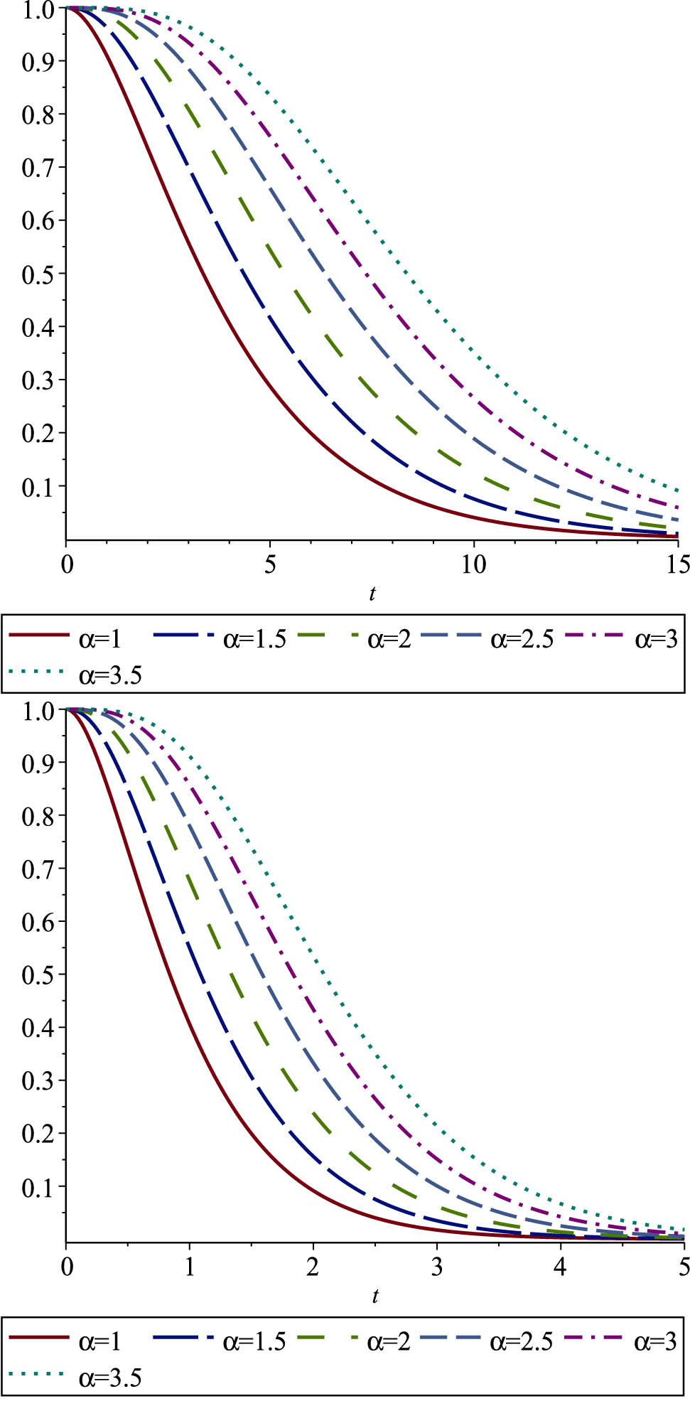
The TSD bound in Theorem 3.4 is decreasing (increasing) in α for 1 / 2 < α ≤ 1 ( α ≥ 1 ) ; however, it can be applied for α > 1 / 2 . While the TRA bound can be applied for all α ∈ D + . So, this bound is a suitable alternative for the case of α < 1 / 2 . The next example delivers these notes.

Example 3.1

Let X ∈ R + have a standard exponential distribution with the survival function S ( x ) = e − x , x > 0 . By considering Ψ ( x ) = x k , k ≥ 1 , we obtain

Π ϕ , β ( X ) = ∫ 0 ∞ ϕ ( x ) S β ( x ) d x = k ∫ 0 ∞ x k − 1 e − β x d x = k Γ ( k ) β k ,

for all β > 0 . To provide an expression for the transformed variance and the WFGCRE of exponential distribution, first note that

m Ψ ( t ) = k e t ∫ t ∞ x k − 1 e − x d x = k e t Γ ( t , k ) ,

where Γ ( t , k ) denotes the upper incomplete gamma function. Now, due to Theorem 3 in ref. [18], we have

σ 2 ( X k ) = ∫ 0 ∞ m Ψ ( t ) e − t d t = Γ ( 1 + 2 k ) − [ Γ ( 1 + k ) ] 2 .

Moreover, Theorem 2.5 implies that

E α Ψ ( X ) = k Γ ( α + k ) Γ ( α + 1 ) .

Now, Theorem 3.4 gives

E α Ψ ( X ) ≤ 1 Γ ( α ) Γ ( 2 α − 1 ) [ Γ ( 1 + 2 k ) − [ Γ ( 1 + k ) ] 2 ] ,

in which α > 1 / 2 . Taking into account

β = α , α ∈ [ 0 , 1 ] 1 α , α ∈ [ 1 , ∞ ) ,

Part (ii) of Theorem 3.4 gives

E α Ψ ( X ) ≤ k α α − k e − α Γ ( k ) ( 1 − α ) α Γ ( α + 1 ) , α ∈ [ 0 , 1 ]

and

E α Ψ ( X ) ≤ k α 2 α + k e − α Γ ( k ) ( α − 1 ) α Γ ( α + 1 ) , α ∈ [ 1 , ∞ ) .

In Figures 2, 3, 4, we depicted the TSD and the TRA bounds as shown in Theorem 3.4 as well as the plot of E α Ψ ( X ) for α ∈ [ 0 , 1 ] in the left panel and for α ∈ [ 1 , ∞ ) in the right panel for k = 1 , 2 , 3 , respectively. For this model, the transformed SD bound is not computed for all k = 1 , 2 , 3 when α ∈ [ 0 , 0.5 ] In this case, when α ∈ [ 0.5 , 1 ] , the TSD bound has better result.

$Figure 2 The TSD (dashed line) and the TRA (dotted line) bounds as well as the exact value of WFGCRE (solid line) for the exponential model for various values of k = 1 k=1 when α ∈ [ 0 , 1 ] \alpha \in \left[0,1] (left) and α ∈ [ 1 , ∞ ) \alpha \in \left[1,\infty ) (right).$

Figure 2

The TSD (dashed line) and the TRA (dotted line) bounds as well as the exact value of WFGCRE (solid line) for the exponential model for various values of k = 1 when α ∈ [ 0 , 1 ] (left) and α ∈ [ 1 , ∞ ) (right).

$Figure 3 The TSD (dashed line) and the TRA (dotted line) bounds as well as the exact value of WFGCRE (solid line) for the exponential model for various values of k = 2 k=2 when α ∈ [ 0 , 1 ] \alpha \in \left[0,1] (left) and α ∈ [ 1 , ∞ ) \alpha \in \left[1,\infty ) (right).$

Figure 3

The TSD (dashed line) and the TRA (dotted line) bounds as well as the exact value of WFGCRE (solid line) for the exponential model for various values of k = 2 when α ∈ [ 0 , 1 ] (left) and α ∈ [ 1 , ∞ ) (right).

$Figure 4 The TSD (dashed line) and the TRA (dotted line) bounds as well as the exact value of WFGCRE (solid line) for the exponential model for various values of k = 3 k=3 when α ∈ [ 0 , 1 ] \alpha \in \left[0,1] (left) and α ∈ [ 1 , ∞ ) \alpha \in \left[1,\infty ) (right).$

Figure 4

The TSD (dashed line) and the TRA (dotted line) bounds as well as the exact value of WFGCRE (solid line) for the exponential model for various values of k = 3 when α ∈ [ 0 , 1 ] (left) and α ∈ [ 1 , ∞ ) (right).

3.2 Stochastic comparisons

Hereafter, we present some ordering properties of the weighted FGCRE. We recall, in general, that the usual stochastic ordering does not imply the ordering of weighted FGCREs. The counterexample 3 in ref. [12] validates this claim. Before beginning the subsequent theorem, we require the next definition due to ref. [18].

Definition 3.1

Let m Ψ ( X 1 ) ( t ) and m Ψ ( X 2 ) ( t ) , be the WMRL functions of X 1 ∈ R + and X 2 ∈ R + , respectively. Further, assume ϕ ( ⋅ ) be a nonnegative weight function. Then, we say that X 1 is smaller than X 2 in the WMRL with respect to the weight function ϕ ( t ) , denoted by X 1 ≤ w m r l ϕ X 2 , if m Ψ ( X 1 ) ( t ) ≤ m Ψ ( X 2 ) ( t ) , for all t ≥ 0 .

Now, we state the next theorem.

Theorem 3.5

Let X 1 , X 2 ∈ R + with CDFs F 1 ( x ) and F 2 ( x ) , and WMRL functions m ψ ( X 1 ) ( t ) and m ψ ( X 2 ) ( t ) , respectively, and such that X 1 ≤ s t X 2 . Then, for all α ∈ D + ,

if X 1 ≤ w m r l ϕ X 2 and either X 1 or X 2 is IWMRL, then E α Ψ ( X 1 ) ≤ E α Ψ ( X 2 ) .
if X 1 ≥ w m r l ϕ X 2 and either X 1 or X 2 is DWMRL, then E α Ψ ( X 1 ) ≥ E α Ψ ( X 2 ) .

Proof

We assume that the survival function of X i , α , i = 1 , 2 , is given by S i , α ( x ) = K α ( S i ( x ) ) , x > 0 . Let X 2 be IWMRL. From (17), we obtain

(23) E 1 , α Ψ ( X 1 ) = E [ m ψ ( X 1 ) ( X 1 , α ) ] ≤ E [ m ψ ( X 2 ) ( X 1 , α ) ] ≤ E [ m ψ ( X 2 ) ( X 2 , α ) ] = E 2 , α Ψ ( X 2 ) .

The first inequality in (23) is given using the assumption X 1 ≤ w m r l ϕ X 2 ; however, the last inequality derives from Lemma 1 in [12] by noting that X 1 ≤ s t X 2 . Now, let X 1 be IWMRL. Then, we similarly have

E 1 , α Ψ ( X 1 ) = E [ m ψ ( X 1 ) ( X 1 , α ) ] ≤ E [ m ψ ( X 1 ) ( X 2 , α ) ] ≤ E [ m ψ ( X 2 ) ( X 2 , α ) ] = E 2 , α Ψ ( X 2 ) .

Hence, the stated results in (i) follow. In a similar manner, Part (ii) can be obtained.□

The following theorem shows identical results under a few distinct hypotheses. The proof is parallel, and hence, it is skipped.

Theorem 3.6

Under the conditions of Theorem 3.5, if X 1 ≤ h r X 2 , and X 1 or X 2 is IWMRL, then E α Ψ ( X 1 ) ≤ E α Ψ ( X 2 ) for all α ∈ D + .

Proof

Let X 1 be IWMRL. From (17), we obtain

E 1 , α Ψ ( X 1 ) = E [ m ψ ( X 1 ) ( X 1 , α ) ] ≤ E [ m ψ ( X 1 ) ( X 2 , α ) ] ≤ E [ m ψ ( X 2 ) ( X 2 , α ) ] = E 2 , α Ψ ( X 2 ) .

It is well known that X 1 ≤ h r X 2 implies X 1 ≤ s t X 2 , and this yields X 1 , α ≤ s t X 2 , α for all for all α ∈ D + due to Lemma 1 in ref. [12], and hence, the first inequality is concluded since m ψ ( X 1 ) ( x ) is increasing. The second inequality is obtained by recalling the relation (42) of ref. [18]. When X 2 is IWMRL, the proof is similar.□

The subsequent outcome is applied with the MRL order. It readily follows from relation (37) in ref. [18].

Corollary 3.1

Under the conditions of Theorem 3.5, it holds that

If X 1 ≤ m r l X 2 and either X 1 or X 2 is IWMRL, then E 1 , α Ψ ( X 1 ) ≤ E 2 , α Ψ ( X 2 ) , for all α ∈ D + .
If X 1 ≥ m r l X 2 and either X 1 or X 2 is DWMRL, then E 1 , α Ψ ( X 1 ) ≥ E 2 , α Ψ ( X 2 ) , for all α ∈ D + .

Hereafter, we provide an application of the aforementioned result. The first one is based on the random minima. To this aim, we assume a discrete nonnegative random variable N , which is independent of random variables X 1 , X 2 , … . Hence, the minimum extreme order statistics is given as X 1 : N = min { X 1 , X 2 , … , X N } . Now, let us see the subsequent theorem.

Theorem 3.7

If ϕ ( x ) is nondecreasing in x, then E α Ψ ( X 1 : N 1 ) ≥ E α Ψ ( X 1 : N 2 ) for all α ∈ D + provided that N 1 ≤ l r N 2 and X is DFR.

Proof

First, we note that X 1 : N 1 ≥ l r X 1 : N 2 yields X 1 : N 1 ≥ h r X 1 : N 2 due to Theorem 2.4 in ref. [21]. Moreover, based on the assumption, X is DFR which implies that either X 1 : N 1 or X 1 : N 2 is DFR (see ref. [22], and this implies the IMRL property. Since ϕ ( x ) is increasing in x , Theorem 2 of ref. [18] yields X 1 : N 1 or X 1 : N 2 is IWMRL. Consequently, Theorem 3.6 finishes the proof.□

4 Conclusion

We have introduced a new measure of entropy, the weighted FGCRE associated with a random lifetime. The new measure has some connections with the weighted fractional Shannon entropy. Stochastic comparisons of distributions over several known stochastic orders were performed using the new measure. The new measure was used to derive the weighted fractional generalized CRE for random minima. Shannon entropy is crucial in several areas of statistical mechanics and information theory. In this case, the notion of entropy as a measure of uncertainty plays a crucial role in statistics, thermodynamics, information theory, and machine learning. In this work, we have defined a new measure of uncertainty given by the weighted fractional generalized residual cumulative entropy of a nonnegative absolutely continuous random variable. We have derived several other properties for this measure, including its various representations, upper and lower bounds for it, and some other useful results.

In the future of this study, the weighted fractional generalized CRE will be used to analyze coherent systems. The study of such systems in the context of information theory and in terms of the new measure proposed in this article will be a useful investigation, since the concept of uncertainty plays a crucial role in the analysis and evaluation of coherent systems in industry and engineering.

Acknowledgments

The authors are very grateful to anonymous reviewers for their careful reading of an earlier version of this article and their useful constructive comments that led to this improved version.

Funding information: Princess Nourah bint Abdulrahman University Researchers Supporting Project number (PNURSP2023R226), Princess Nourah bint Abdulrahman University, Riyadh, Saudi Arabia.
Author contributions: All authors have accepted responsibility for the entire content of this article and approved its submission.
Conflict of interest: The authors state no conflict of interest.

References

[1] Nascimento JPG, Ferreira FAP, Aguiar V, Guedes I, CostaFilho RN. Information measures of a deformed harmonic oscillator in a static electric field. Phys A Stat Mech Appl. 2018 Jun;499:250–7. 10.1016/j.physa.2018.02.036Search in Google Scholar

[2] Srivastava A, Kaur L. Uncertainty and negation—Information theoretic applications. Int J Intell Syst. 2019 Feb;34(6):1248–60. 10.1002/int.22094Search in Google Scholar

[3] Ostovare M, Shahraki MR. Evaluation of hotel websites using the multicriteria analysis of PROMETHEE and GAIA: evidence from the five-star hotels of Mashhad. Tour Manag Perspect. 2019 Apr;30:107–16. 10.1016/j.tmp.2019.02.013Search in Google Scholar

[4] Tang Y, Chen Y, Zhou D. Measuring uncertainty in the negation evidence for multi-source information fusion. Entropy. 2022 Nov 2;24(11):1596. 10.3390/e24111596Search in Google Scholar PubMed PubMed Central

[5] Ubriaco MR. Entropies based on fractional calculus. Phys Lett A. 2009 Jul;373(30):2516–9. 10.1016/j.physleta.2009.05.026Search in Google Scholar

[6] Shannon CE, Weaver W. The mathematical theory of communication. Math Gaz. 1949 Dec;34(310):312. Search in Google Scholar

[7] Guiaşu S. Weighted entropy. Rep Math Phys. 1971 Sep;2(3):165–79. 10.1016/0034-4877(71)90002-4Search in Google Scholar

[8] Rao M, Chen Y, Vemuri BC, Wang F. Cumulative residual entropy: a new measure of information. IEEE Trans Inf Theory. 2004 Jun;50(6):1220–8. 10.1109/TIT.2004.828057Search in Google Scholar

[9] Xiong H, Shang P, Zhang Y. Fractional cumulative residual entropy. Commun Nonlinear Sci. 2019 Nov;78:104879. 10.1016/j.cnsns.2019.104879Search in Google Scholar

[10] DiCrescenzo A, Kayal S, Meoli A. Fractional generalized cumulative entropy and its dynamic version. Commun Nonlinear Sci. 2021 Nov;102:105899. 10.1016/j.cnsns.2021.105899Search in Google Scholar

[11] Alomani G, Kayid M. Fractional survival functional entropy of engineering systems. Entropy. 2022 Sep 10;24(9):1275. 10.3390/e24091275Search in Google Scholar PubMed PubMed Central

[12] Alomani G, Kayid M. Stochastic properties of fractional generalized cumulative residual entropy and its extensions. Entropy. 2022 Jul 28;24(8):1041. 10.3390/e24081041Search in Google Scholar PubMed PubMed Central

[13] Psarrakos G, Economou P. On the generalized cumulative residual entropy weighted distributions. Commun Stat Theory Meth. 2016 Nov 2;46(22):10914–25. 10.1080/03610926.2016.1252402Search in Google Scholar

[14] Toomaj A, Sunoj SM, Navarro J. Some properties of the cumulative residual entropy of coherent and mixed systems. J Appl Probab. 2017 Jun;54(2):379–93. 10.1017/jpr.2017.6Search in Google Scholar

[15] Psarrakos G, Toomaj A. On the generalized cumulative residual entropy with applications in actuarial science. J Comput Appl Math. 2017 Jan;309:186–99. 10.1016/j.cam.2016.06.037Search in Google Scholar

[16] Toomaj A, Atabay HA. Some new findings on the cumulative residual Tsallis entropy. J Comput Appl Math. 2022 Jan;400:113669. 10.1016/j.cam.2021.113669Search in Google Scholar

[17] Shaked M, George Shanthikumar J. Stochastic orders. New York, London: Springer; 2011. Search in Google Scholar

[18] Toomaj A, Di Crescenzo A. Connections between weighted generalized cumulative residual entropy and variance. Mathematics. 2020 July 2;8(7):1072. 10.3390/math8071072Search in Google Scholar

[19] Asadi M, Ebrahimi N. Residual entropy and its characterizations in terms of hazard function and mean residual life function. Stat Probab Lett. 2000 Sep;49(3):263–9. 10.1016/S0167-7152(00)00056-0Search in Google Scholar

[20] Wang S. Insurance pricing and increased limits rate making by proportional hazards transforms. Insur Math Econ. 1995 Aug;17(1):43–54. 10.1016/0167-6687(95)00010-PSearch in Google Scholar

[21] Shaked M, Wong T. Stochastic orders based on ratios of Laplace transforms. J Appl Probab. 1997 Jun;34(2):404–19. 10.2307/3215380Search in Google Scholar

[22] Shaked M. On the distribution of the minimum and of the maximum of a random number of iid random variables. In: A modern course on statistical distributions in scientific work. Springer; 1975. p. 363–80. 10.1007/978-94-010-1842-5_29Search in Google Scholar

Received: 2022-10-26

Revised: 2023-02-07

Accepted: 2023-02-15

Published Online: 2023-03-04

This work is licensed under the Creative Commons Attribution 4.0 International License.

Articles in the same Issue

https://doi.org/10.1515/phys-2022-0234

Keywords for this article

weighted fractional generalized cumulative residual entropy; generalized cumulative residual entropy; weighted mean residual lifetime; stochastic orders

Creative Commons

BY 4.0