Optimal interatomic potentials using modified method of least squares: Optimal form of interatomic potentials

1 Introduction

Phenomenological potential functions [1] are well known to describe the interactions (or forces) between neighbour and/or adjacent atoms [2]. It is therefore necessary to select a potential function that is most appropriate towards the intended aim of the particular experiment(s) or computational software. Although, in quantum mechanics, the Lennard–Jones potential seems to be the most preferred potential. We will be confirming this hypothesis by classifying selected potentials, and after performing a one-dimensional search, the most appropriate potential will be proposed. Interatomic potentials theory is a field of study teeming with possibilities due to its modern applications in quantum mechanics [3], nanotechnology, and nanoengineering [1]. In this modern times, a lot of scientific effort has been channelled towards proposing and modifying interatomic potentials for greater computational efficiency. Between interatomic potentials, we often meet with phenomenological potentials having the generalized mathematical representation

where U ˜ ( ρ ) = U ˜ is the interatomic potential depending on ρ = ρ ( r ) -function of the interatomic distance, r . A , − B > 0 are scalars as well as α > β > 0 , which are scalar exponents. The interatomic distance, ρ = ρ ( r ) , largely determines which potential will result from the generalized representation in Eq. (1). For example, at ρ ( r ) = r , the classical Morse potential

will be obtained. In potential (2), A = ε e 2 β r m , B = − 2 ε e β r m , ε is the depth of the energy minimum, r m is the corresponding minimum value of equilibrium distance between two atoms, and β is the steepness of the negative exponent term. At the same ρ ( r ) = r , the generalized Morse potential, which is also mentioned in the study by Teik-Cheng [4] as the Biswas-Hamann potential [5,6],

will be obtained. Finally, the classical Rydberg potential [5,6]

is also obtainable. The original form of this potential was proposed in the study by Rydberg [7]. Potentials presented in Eqs. (2)–(4) are referred to as the second-order potentials because they can be treated as solutions of the second-order homogeneous ordinary differential equation (ODE)

where ρ = ρ ( r ) , e.g., ρ = r , ρ = ln r , ρ = r 2 . Values of a and b are dependent on Eqs. (2), (3), or (4).

Eigenvalues of ODE (5) are obtained from the characteristic equation, λ 2 + a λ + b = 0 and are

where a = α + β > 0 , b = α ⋅ β > 0 . If a 2 − 4 b > 0 , and then we obtain the generalized Morse potential (3), with

In a particular case where α = 2 β , we will obtain the classical Morse potential, (2). This situation is realized at 2 a 2 = 9 b in ODE (5). Another particular situation in ODE (5), arises when a 2 = 4 b . In this case, the interatomic potential has the classical Rydberg form (4).

In the previously analyzed cases, we considered only instances where a 2 − 4 b ≥ 0 . It is worthwhile to consider a situation with a 2 − 4 b < 0 . In this case, the interatomic potential is described in a real form as follows:

where δ = − a 2 and ω = − 4 b − a 2 2 . Potential (7) was referred to as the modified generalized Morse potential in [8]. Other different forms of the function, ρ = ρ ( r ) , will also give some other classical interatomic potentials. For example, at ρ ( r ) = ln r , we will obtain

which is the generalized Lennard–Jones potential [4,9], originally proposed by Jones [9]. In particular case, at α = 12 and β = 6 , we have the well-known classical 12 − 6 Lennard–Jones potential. Considering another example, at ρ ( r ) = r 2 , we have the two-body portion of the Kaxiras–Pandey potential function [10,11]

Elaborate discussions on the theory of interatomic potentials are extensively detailed in previous studies [1,12–15]. In tandem with formula (8), let us propose analogues of the Lennard–Jones-Rydberg potential

and along with formula (7), let us also propose the analogue of the modified Morse–Lennard–Jones potential

Analogously, we propose further generalizations of the Kaxiras–Pandey potential (9) in the following forms as the Kaxiras–Pandey–Rydberg potential

and the modified Morse–Kaxiras–Pandey potential

All these potentials were previously considered as functions with real values of parameters [8,16– 25,27]. The first generalization of the previously mentioned potentials is being presented in this article, where potentials (3), (8), and (9) were considered for both real and complex conjugate pairs α , β , A , and B . This point of view is a substantial breakthrough because it increases the domain in which the values of parameters are being searched. This generalization directly follows from the proposed approach in the frames of which the functional forms of the potentials are considered as possible solutions of the second-order ODE (5) with constant (real) values a , b . The research question we seek to answer in this article is: What is the most appropriate form of ρ = ρ ( r ) − function of the interatomic distance, r ? Such that this optimal potential will enable nano-scientists to adequately observe interactions at the atomic level, and make sound judgments or conclusions from their studies. To answer this question, we will formulate a generalized form for each of the three forms of ρ = ρ ( r ) previously discussed and use the method of least squares to estimate the unknown parameter, γ , of the generalized potentials.

2 Formulation of the optimization problem

Synthesizing the previous mathematical representations, let us now formulate the problem of optimization of the phenomenological interatomic potential representation in either Lennard–Jones forms (8), (10), or (11). We can rather consider the forms

where we considered ρ = ρ ( r ) as ρ = r γ and γ is the parameter subjected to optimization. Alternatively, we can also consider the synthesized form

or

Let us remark that (14)–(16) can be treated as solutions of the ODE

or after change of variables ρ = r γ by ODE (5). In this case, we use form (14) if α and β are real and different; form (15) if α ≈ β > 0 , and form (16) if eigenvalues in ODE (5) are complex conjugates, λ 1 , 2 = δ ± i ω ( i 2 = − 1 ) , where δ = Re ( λ 1 , 2 ) and ω = ∣ Im ( λ 1 , 2 ) ∣ .

We formulate the problem of optimization of the parameter representation of the interatomic potential as follows:

where U i exp = U exp ( r i ) are the experimental values of the potential at interatomic distance, r = r i . To solve this problem, we select interval of values of parameter γ ∈ [ γ min , γ max ] , divide it by M subintervals, calculate, and then we minimize the function G at every value

for m = 0 , 1 , … , M . Further, we recalculate r i ⟶ ρ i = r i γ m and integrate ODE (5) from ρ min to ρ

where U ˜ min = U ˜ ( ρ = ρ min ) and U ˜ ′ ( ρ ) = d U ˜ ( ρ ) d ρ . Integrated ODE (19) can also be expressed as follows:

where I ˜ 1 ( ρ ) = ∫ ρ min ρ U ˜ ( σ ) d σ , and c = − ( U ˜ ′ min + a U ˜ min ) are the new unknown parameters. After the second integration, we obtain

where Δ U ˜ ( ρ ) = U ˜ ( ρ ) − U ˜ min , I ˜ 2 ( ρ ) = ∫ ρ min ρ I ˜ 1 ( σ ) d σ , Δ ρ ˜ = ρ − ρ min . Model (21) is linear with respect to unknown parameters a , b , and c , which are calculated using the least squares method through the goal function minimization:

where I 1 , i = I ˜ 1 ( ρ i ) , I 2 , i = I ˜ 2 ( ρ i ) , Δ ρ i = ρ i − ρ min , Δ U i = Δ U ˜ ( ρ i ) . The solution of this problem is

where M 1 = [ I 1 I 2 Δ ρ ] is ( N × 3 ) matrix, I 1 = ( I 1 , i ) , I 2 = ( I 2 , i ) , Δ ρ = ( Δ ρ i ) and Δ U = ( Δ U i ) are ( N × 1 ) − columns. System (23) was obtained by partially differentiating goal function (22) with respect to a , b , c , setting the derivatives to 0 and writing the resulting equations in the matrix form.

By calculating eigenvalues λ 1 , 2 using formula (6), we make a choice between the representations (14)–(16). Namely, if λ 1 and λ 2 are real and well separated, we use (14); if they are complex conjugates, we use (16). If λ 1 and λ 2 are close to each other, it is reasonable to use representation (15). To find the proper value of α in (15), it is worthwhile to repeat the procedure of the algorithm explained by Kikawa et al. [22], for the classical Rydberg potential identification.

Next step involves definition of parameters A and B in (14)–(16). In this case, we use basic functions f ˜ 1 ( r ) and f ˜ 2 ( r ) , which are equal to

In this case, the general representation of formulas (14)–(16) reduces to:

and the second goal function, which is subjected to minimization is:

The solution of this conventional problem is

where M 2 = [ f 1 f 2 ] is ( N × 2 ) matrix, and f 1 = ( f 1 , i ) , f 2 = ( f 2 , i ) , and U = ( U i ) are ( N × 1 ) -vector-columns.

Repeating this algorithm M times for the selected γ m ( m = 1 , 2 , … , M ) , we find γ ˜ min = min ( m ) ( γ m ) . This value can be used as guess value for further search of the optimal value of γ . It is also possible to round γ ˜ min to the closest integer for faster calculations of values of the interpolated interatomic potential.

As we have explained earlier, γ can be 1 (like in the case of generalized Morse, classical Morse, and classical Rydberg potentials); can be 2 (like in the case of Kaxiras–Pandey potential and it’s analogues); or can also be 3 for some modified potentials. The treatment of all potentials as solutions of the corresponding ODE (5) immediately defines the form of the potential and domain (real or complex) for its parameters. Moreover, ODE (5) is linear with respect to parameters a and b , which guarantees unique solution to the problem of determination of exponential parameters α and β . This is the novelty of the presented research instead of the conventional “brute force” fitting of the original transcendent potentials. It is necessary to mention that this fitting is performed on the last stage of fitting when the guess values of the parameters are determined by means of the subtle method of minimization of two quadratic goal functions, which was previously formulated in [26] and has been extensively used by the authors in previous studies [8,16– 25,27].

3 Numerical simulations

In what follows, we will be performing numerical simulations of goal functions (18), (22), and (26). We will start by first assuming numerical values for the parameter, γ , to be γ = 0.5 or 3; then we obtain estimates for α and β , and use these estimates to calculate the estimates for A and B . Finally, we carry out the one-dimensional search in order to determine the most appropriate value of γ . The process will be carried out for experimental data sets of metals such as gold [28], copper [29], aluminium [30], titanium [30], and copper–silver alloy [29]. The experimental data sets of the metals were downloaded from the online repository, Interatomic Potentials Repository website^[1]. The form of the interatomic potentials considered has already been presented in Eqs. (14)–(16). It should be noted that the closer the values of the goal function to 0, the more accurate the parameter estimates are. The closer the goal function values are to 1, the more inaccurate the parameter estimates are. For gold atoms [28], and γ = 0.5 , the following values were obtained

hence, α = 12.36613 and β = 5.79498 . The form (14) is preferred since both values are real, and distinct. Numerical simulations then yield A = 2.00117 × 1 0 8 , and B = − 4.94973 × 1 0 3 . The one-dimensional search for parameter, γ (steepest point of the presented curve), yielded γ = 0.38847 (estimated from Figure 1)

Figure 1

One-dimensional search for parameter, γ , using gold atoms.

When we considered the form, ρ ( r ) = ln r , for the Lennard–Jones potential and its analogues, the following values were obtained

The estimated value for parameter γ was then used to construct and reconstruct potential energy curves (PECs) using downloaded experimental data sets of gold atoms and parameter values fitted to potential (14).

The error curves between the two PECs in Figure 2 shows a dimension of magnitude 4 × 1 0 − 3 . In Figure 2 (and other subsequent figures), U n represents the fitted experimental data, U U U n represents the fitted estimated parameters, while ρ n represents the interatomic distance. For copper atoms [29], and γ = 3 , the following values were obtained

therefore, α = 0.35283 and β = 0.04893 . The form (14) is preferred since α and β are real, and distinct. Hence, A = 18.66203 and B = − 0.50888 . The one-dimensional search for parameter, γ (steepest point of the presented curve), yielded γ = 0.01659

Figure 2

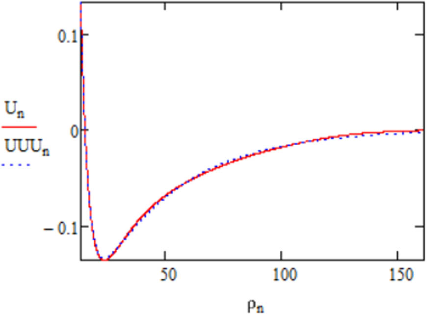
Comparison of PECs for original data sets and estimated parameters.

From Figure 3, we can infer that the minimum of the optimized goal function has two values, 0 or 3 . This means we can use ρ ( r ) = r γ , where γ = 3 , or we could also use ρ ( r ) = ln r for the optimal potential. In principle, it will be more efficient to use ρ ( r ) = ln r . When we considered the form, ρ ( r ) = ln r , for the Lennard–Jones potential and its analogues, the following values were obtained

The estimated values using ρ ( r ) = ln r was then used to construct and reconstruct, PECs using experimental data sets of copper atoms and parameter values.

Figure 3

One-dimensional search for parameter, γ , using copper atoms.

The error curves between the two PECs in Figure 4 shows a dimension of magnitude 1 × 1 0 − 3 . For aluminium atoms [30], and γ = 3 , the following values were obtained

therefore, α = 0.19517 , β = 0.04052 . The form (14) is preferred since α and β are real, and distinct. Hence, A = 6.06236 and B = 0.92577 . The one-dimensional search for parameter, γ , yielded γ = 1.43507 .

Figure 4

Comparison of PECs for original data sets and estimated parameters.

In the case of Figure 5, the minimum lies between 1 and 2. Hence, γ = 1 or 2 can be used. This means for aluminium atoms, the optimal potential is either the generalized Morse or the Kaxiras–Pandey potential. When we considered the form, ρ ( r ) = ln r , for the Lennard–Jones potential and its analogues, the following values were obtained

The estimated value for parameter γ was then used to construct and reconstruct PECs using experimental data sets of aluminium atoms and parameter values.

Figure 5

One-dimensional search for parameter, γ , using aluminium atoms.

The error curves between the two PECs in Figure 6 shows a dimension of magnitude 2 × 1 0 − 2 . For titanium atoms [30], and γ = 3 , the following values were obtained

therefore, α = 0.25529 and β = 0.03544 . The form (14) is preferred since α and β are real, and distinct. Hence, A = 22.14025 and B = − 2.47284 . The one-dimensional search for parameter, γ , yielded γ = 0.16645 .

Figure 6

Comparison of PECs for original data sets and estimated parameters.

Figure 7 shows the optimized goal function having a minimum of γ ≈ 0 , which means the optimal potential is obtained when ρ ( r ) = ln r . When we considered the form, ρ ( r ) = ln r , for the Lennard–Jones potential and its analogues, the following values were obtained

The estimated value for parameter γ was then used to construct and reconstruct PECs using experimental data sets of titanium atoms and parameter values fitted to potential.

Figure 7

One-dimensional search for parameter, γ , using titanium atoms.

The error curves between the two PECs in Figure 8 shows a dimension of magnitude 2 × 1 0 − 2 . Finally, when we analyze the silver–copper alloy [29], with γ = 3 , the following values were obtained

therefore, α = 0.31588 , and β = 0.02722 . The form (14) is preferred since α and β are real, and distinct. Hence, A = 24.46179 and B = − 0.28071 . The one-dimensional search for parameter, γ , yielded γ = 2.98832 (estimated from Figure 9).

Figure 8

Comparison of PECs for original data sets and estimated parameters.

Figure 9

One-dimensional search for parameter, γ , using silver–copper alloy.

Without a doubt, the optimal potential for silver–copper alloy is realized when γ = 3 . This potential will be an analogues or a modification of the generalized Morse potential. When we considered the form, ρ ( r ) = ln r , for the Lennard–Jones potential and its analogues, the following values were obtained

The estimated value for parameter γ was then used to construct and reconstruct PECs using experimental data sets and parameter values.

The error curves between the two PECs in Figure 10 shows a dimension of magnitude 2 × 1 0 − 3 . As was graphically illustrated in Figures 2, 4, 6, 8, and 10, the obtained parameter estimates for α , β , A , and B used to plot PECs, all showed reasonable agreement with the experimental data sets. The obtained PECs were graphically indistinguishable through a large range of the interatomic distance, r . Table 1 illustrates the values of the goal function for both forms of ρ ( r ) considered and for each metal atoms used for experimental values. It should be recalled that the closer the numerical values are to 0, the more accurate the parameter estimates calculated.

Figure 10

Comparison of PECs for original data sets and estimated parameters.

The goal function values were obtained by minimizing the goal functions (26) and (18) through built in functions in Mathcad^®.

Table 2 concisely summarizes the results obtained from numerical simulations. The preferred choice of potential used for numerical simulation was based on the agreement of the reconstructed PECs with experimental data sets.

4 Discussion and conclusion

In this article, interatomic potentials that can be treated as solutions of some second-order ODE were classified and identified. A generalization of three forms of potentials were presented, and the most appropriate form of a generalized potential will be based on the estimated value of parameter, γ . The goal function values were also stated in Table 1. Reconstructed PECs showed good agreement for a relatively large vicinity of the potential minimum, between the estimates and experimental data sets. It should be noted that there are two ways of optimization: the first one relates to the selection of the “ γ ” exponent. (In the available literature, the authors used γ = 1 for the generalized Morse potential [4] and γ = 2 for the Kaxiras–Pandey potential [10,11]. The question is why not γ = 3 2 , for example, or some other value?.) The second optimization relates to either real or complex conjugate exponents and the corresponding factors (in the direct brute force optimisation, it is impossible to change the field of real valued parameters to the field of complex conjugate ones, it is possible only in the frames of the authors approach using the multiple (double) goal functions method).

In general, we can infer that the form with Lennard–Jones potential has the lower goal function values and hence is the optimal interatomic potential (most preferable potential), for many cases. The one-dimensional search for the most appropriate value of the parameter, γ , fails when copper, titanium, and aluminium were analyzed. However, this defect does not affect the reconstructed PECs. Having performed numerical simulations using different values of γ , we can also infer that when γ = 3 , the optimal potential is obtained and is more preferable as compared to other cases when γ = 1 or 2.

References

[1] Rieth M. Nano-engineering in science and technology: an introduction to the world of nano-design. United Kingdom: World Scientific; 2003. 10.1142/5026Search in Google Scholar
[2] Torrens IM. Interatomic potentials. New York, United States: Academic Press Inc.; 1972. 10.1016/B978-0-12-695850-8.50010-5Search in Google Scholar
[3] Mitin VV, Sementsov DI, Vagidov NZ. Quantum mechanics for nanostructures. United Kingdom: Cambridge University Press; 2010. 10.1017/CBO9780511845161Search in Google Scholar
[4] Teik-Cheng L. Relationship and discrepancies among typical interatomic potential functions. Chinese Phys Lett. 2004;21(11):2167. 10.1088/0256-307X/21/11/025Search in Google Scholar
[5] Biswas R, Hamann D. New classical models for silicon structural energies. Phys Rev B. 1987;36(12):6434. 10.1103/PhysRevB.36.6434Search in Google Scholar PubMed
[6] Murrell JN, Sorbie KS. New analytic form for the potential energy curves of stable diatomic states. J Chem Soc Faraday Trans 2. 1974;70:1552–6. 10.1039/f29747001552Search in Google Scholar
[7] Rydberg R. Graphische darstellung einiger bandenspektroskopischer ergebnisse. Z Phys A Hadrons Nucl. 1932;73(5):376–85. 10.1007/BF01341146Search in Google Scholar
[8] Surulere SA, Mkolesia AC, Shatalov MY, Fedotov IA. A modern approach for the identification of the classical and modified generalized morse potential. Nanosci Nanotech Asia. 2020;10(2):142–51. 10.2174/2210681208666181010141842Search in Google Scholar
[9] Jones JE. On the determination of molecular fields. II. from the equation of state of a gas. In: Proceedings of the Royal Society of London A: Mathematical, Physical and Engineering Sciences. Vol. 106. 1924. p. 463–77. 10.1098/rspa.1924.0082Search in Google Scholar
[10] Kaxiras E, Pandey K. New classical potential for accurate simulation of atomic processes in Si. Phys Rev B. 1988;38(17):12736. 10.1103/PhysRevB.38.12736Search in Google Scholar PubMed
[11] Lim TC. Connection between the 2-body energy of the Kaxiras–Pandey and the Biswas-Hamann potentials. Czechoslovak J Phys. 2004;54(9):947–63. 10.1023/B:CJOP.0000042647.51651.2aSearch in Google Scholar
[12] Bartók-Pártay A. The Gaussian approximation potential: an interatomic potential derived from first principles quantum mechanics. Heidelberg, Germany: Springer Science & Business Media; 2010. 10.1007/978-3-642-14067-9_4Search in Google Scholar
[13] Brenner D. The art and science of an analytic potential. Physica Status Solidi (b). 2000;217(1):23–40. 10.1002/(SICI)1521-3951(200001)217:1<23::AID-PSSB23>3.0.CO;2-NSearch in Google Scholar
[14] Kaplan IG. Intermolecular interactions: physical picture, computational methods and model potentials. New Jersey, United States: John Wiley & Sons; 2006. 10.1002/047086334XSearch in Google Scholar
[15] Rafii-Tabar H, Mansoori G. Interatomic potential models for nanostructures. Encyclopedia Nanosci Nanotech. 2004;6:231–47. Search in Google Scholar
[16] Surulere SA. The investigation of vibrations in a linear and nonlinear continuum of atoms. PhD thesis, Tshwane University of Technology, South Africa; 2021. Search in Google Scholar
[17] Surulere SA, Shatalov MY, Mkolesia AC, Malange T, Adeniji AA. The integral-differential and integral approach for the exact solution of the hybrid functional forms for Morse potential. IAENG Int J Appl Math. 2020;50(2):242–50. Search in Google Scholar
[18] Surulere SA, Shatalov MY, Mkolesia AC, Ehigie JO. The integral-differential and integral approach for the estimation of the classical Lennard–Jones and Biswas-Hamann potentials. Int J Math Model Numer Optim. 2020;10(3):239–54. 10.1504/IJMMNO.2020.108612Search in Google Scholar
[19] Surulere SA, Malange T, Shatalov MY, Mkolesia AC. Parameter estimation of potentials that are solutions of some second-order ordinary differential equation. Discontinuity Nonlinearity Complexity. 2021;12(1):207–29. 10.5890/DNC.2023.03.015Search in Google Scholar
[20] Malange T, Surulere SA, Shatalov MY, Mkolesia AC. Method of characteristic points for composite Rydberg interatomic potential. Int J Comput Sci Math. 2023;18(1):32–43. 10.1504/IJCSM.2023.10059127Search in Google Scholar
[21] Surulere SA. Investigation of the vibrations of linearly growing nanostructures. Master’s thesis. South Africa: Tshwane University of Technology; 2018. Search in Google Scholar
[22] Kikawa CR, Malange T, Shatalov MY, Joubert SV. Identification of the Rydberg interatomic potential for problems of nanotechnology. J Comput Theoret Nanosci. 2016;13(7):4649–55. 10.1166/jctn.2016.5331Search in Google Scholar
[23] Kikawa CR, Shatalov MY, Kloppers PH. Exact solutions for the generalized Morse interatomic potential via the least-squares method. Transylvanian Rev. 2016;24(6):630–5. Search in Google Scholar
[24] Kikawa CR, Shatalov MY, Kloppers PH. A method for computing initial approximations for a 3-parameter exponential function. Phys Sci Int J. 2015;6:203–8. 10.9734/PSIJ/2015/16503Search in Google Scholar
[25] Surulere SA, Shatalov MY, Mkolesia AC, Ehigie JO. A novel identification of the extended-Rydberg potential energy function. Comput Math Math Phys. 2019;59(8):1351–60. 10.1134/S0965542519080153Search in Google Scholar
[26] Kikawa CR. Methods to solve transcendental least-squares problems and their statistical inferences. Unpublished Ph.D. thesis. South Africa: Tshwane University of Technology; 2013. Search in Google Scholar
[27] Malange T. Alternative parameter estimation methods of the classical Rydberg interatomic potential. Master’s thesis. Tshwane: Tshwane University of Technology; 2016. Search in Google Scholar
[28] Olsson PAT. Transverse resonant properties of strained gold nanowires. J Appl Phys. 2010;108(3):034318. 10.1063/1.3460127Search in Google Scholar
[29] Williams P, Mishin Y, Hamilton J. An embedded-atom potential for the Cu-Ag system. Model Simulat Materials Sci Eng. 2006;14(5):817. 10.1088/0965-0393/14/5/002Search in Google Scholar
[30] Zope RR, Mishin Y. Interatomic potentials for atomistic simulations of the Ti-Al system. Phys Rev B. 2003;68(2):024102. 10.1103/PhysRevB.68.024102Search in Google Scholar
© 2023 the author(s), published by De Gruyter
This work is licensed under the Creative Commons Attribution 4.0 International License.
Articles in the same Issue
- Regular Articles
- Dynamic properties of the attachment oscillator arising in the nanophysics
- Parametric simulation of stagnation point flow of motile microorganism hybrid nanofluid across a circular cylinder with sinusoidal radius
- Fractal-fractional advection–diffusion–reaction equations by Ritz approximation approach
- Behaviour and onset of low-dimensional chaos with a periodically varying loss in single-mode homogeneously broadened laser
- Ammonia gas-sensing behavior of uniform nanostructured PPy film prepared by simple-straightforward in situ chemical vapor oxidation
- Analysis of the working mechanism and detection sensitivity of a flash detector
- Flat and bent branes with inner structure in two-field mimetic gravity
- Heat transfer analysis of the MHD stagnation-point flow of third-grade fluid over a porous sheet with thermal radiation effect: An algorithmic approach
- Weighted survival functional entropy and its properties
- Bioconvection effect in the Carreau nanofluid with Cattaneo–Christov heat flux using stagnation point flow in the entropy generation: Micromachines level study
- Study on the impulse mechanism of optical films formed by laser plasma shock waves
- Analysis of sweeping jet and film composite cooling using the decoupled model
- Research on the influence of trapezoidal magnetization of bonded magnetic ring on cogging torque
- Tripartite entanglement and entanglement transfer in a hybrid cavity magnomechanical system
- Compounded Bell-G class of statistical models with applications to COVID-19 and actuarial data
- Degradation of Vibrio cholerae from drinking water by the underwater capillary discharge
- Multiple Lie symmetry solutions for effects of viscous on magnetohydrodynamic flow and heat transfer in non-Newtonian thin film
- Thermal characterization of heat source (sink) on hybridized (Cu–Ag/EG) nanofluid flow via solid stretchable sheet
- Optimizing condition monitoring of ball bearings: An integrated approach using decision tree and extreme learning machine for effective decision-making
- Study on the inter-porosity transfer rate and producing degree of matrix in fractured-porous gas reservoirs
- Interstellar radiation as a Maxwell field: Improved numerical scheme and application to the spectral energy density
- Numerical study of hybridized Williamson nanofluid flow with TC4 and Nichrome over an extending surface
- Controlling the physical field using the shape function technique
- Significance of heat and mass transport in peristaltic flow of Jeffrey material subject to chemical reaction and radiation phenomenon through a tapered channel
- Complex dynamics of a sub-quadratic Lorenz-like system
- Stability control in a helicoidal spin–orbit-coupled open Bose–Bose mixture
- Research on WPD and DBSCAN-L-ISOMAP for circuit fault feature extraction
- Simulation for formation process of atomic orbitals by the finite difference time domain method based on the eight-element Dirac equation
- A modified power-law model: Properties, estimation, and applications
- Bayesian and non-Bayesian estimation of dynamic cumulative residual Tsallis entropy for moment exponential distribution under progressive censored type II
- Computational analysis and biomechanical study of Oldroyd-B fluid with homogeneous and heterogeneous reactions through a vertical non-uniform channel
- Predictability of machine learning framework in cross-section data
- Chaotic characteristics and mixing performance of pseudoplastic fluids in a stirred tank
- Isomorphic shut form valuation for quantum field theory and biological population models
- Vibration sensitivity minimization of an ultra-stable optical reference cavity based on orthogonal experimental design
- Effect of dysprosium on the radiation-shielding features of SiO2–PbO–B2O3 glasses
- Asymptotic formulations of anti-plane problems in pre-stressed compressible elastic laminates
- A study on soliton, lump solutions to a generalized (3+1)-dimensional Hirota--Satsuma--Ito equation
- Tangential electrostatic field at metal surfaces
- Bioconvective gyrotactic microorganisms in third-grade nanofluid flow over a Riga surface with stratification: An approach to entropy minimization
- Infrared spectroscopy for ageing assessment of insulating oils via dielectric loss factor and interfacial tension
- Influence of cationic surfactants on the growth of gypsum crystals
- Study on instability mechanism of KCl/PHPA drilling waste fluid
- Analytical solutions of the extended Kadomtsev–Petviashvili equation in nonlinear media
- A novel compact highly sensitive non-invasive microwave antenna sensor for blood glucose monitoring
- Inspection of Couette and pressure-driven Poiseuille entropy-optimized dissipated flow in a suction/injection horizontal channel: Analytical solutions
- Conserved vectors and solutions of the two-dimensional potential KP equation
- The reciprocal linear effect, a new optical effect of the Sagnac type