Simulation for formation process of atomic orbitals by the finite difference time domain method based on the eight-element Dirac equation
-
Hideki Mutoh


Abstract
Using the finite difference time domain (FDTD) method based on the eight-element Dirac equation, we found that a stable Dirac field wave packet with low velocity can be created without explicit consideration of Zitterbewegung (the rapid oscillatory motion of elementary particles), which is difficult in one-dimensional simulations. Furthermore, we successfully simulated the formation process of atomic orbitals for the first time without any physical approximations by calculating the eight-element Dirac field propagation in the central electric force potential. Initially, a small unstable orbital appears, which rapidly grows and results in a large stable orbital with a radius equal to the Bohr radius divided by the atomic number, as given by the solution of the Schrödinger equation. The FDTD calculation based on the conventional four-element Dirac equation cannot produce such reasonable orbitals owing to the spatial asymmetry of the
1 Introduction
Transient analyses of spatial distributions of atomic and molecular orbitals are crucial for understanding chemical reactions. Experimental investigations of molecular orbitals and their time-dependent spatial distributions have been conducted using Penning ionization electron spectroscopy [1–10], photoelectron spectroscopy with angular distribution [11–15], and electron momentum spectroscopy [16–21]. By contrast, theoretical studies of molecular orbitals have primarily focused on the Schrödinger equation [22–30]. Considering that the orbital spatial distributions change rapidly occurring on a timescale comparable to the orbital length divided by the speed of light, it is essential to solve the Dirac equation instead of the Schrödinger equation for more accurate analyses of the time-dependent spatial distributions of atomic and molecular orbitals. The finite difference time domain (FDTD) method [31,32], which can be used for transient analysis of electromagnetic fields, could also be used for analyzing the Dirac field [33,34] as the Dirac equation is almost equivalent to Maxwell’s equations, except for electron charge and mass [35,36]. In this study, we demonstrate that the FDTD method based on the eight-element Dirac equation successfully calculates the time-dependent Dirac field. Moreover, it reveals the first-ever simulation of the formation process of atomic orbitals, starting from the initial state of a free electron and an atomic nucleus without any physical approximations. This is achieved by calculating the eight-element Dirac field propagation in the central electric force potential.
2 Eight-element Dirac equation
The Dirac equation is given by:
where
For example, gamma matrices are given by:
These matrices have spatial asymmetry, which means that only one or two of
where
where
where
Now, we define matrices
where
Eq. (4) is rewritten as:
Then, we obtain
When
Here, we define four current
Now, we define
Then, we obtain
Therefore,
Next, we consider spin. When we introduce
Eq. (11) is rewritten as:
Under vector potential
Considering the nonrelativistic condition,
where
Therefore, the second term of the right side of the aforementioned equation shows the magnetic moment
we obtain
Therefore,
3 Dirac field propagation analysis by FDTD method
The FDTD method is one of the simplest methods for transient analysis of field propagation, because it can give field spatial distribution dependence on time by only substituting a pair of field vectors each other to discretized equations starting from a given initial state. Since the Dirac equation is quite similar to Maxwell’s equations, the Dirac field propagation could be calculated by the FDTD method, which is popularly used for propagation analysis of electromagnetic field. We compared the calculation results of the FDTD method based on the 1D-like two-element, the conventional four-element, and the extended eight-element Dirac equations. Figure 1 shows the analyzed structure consisting of a cube with a side length
where
k and

Analyzed structure.
3.1 Discretization for the two- and four-element Dirac equation
The four-element Dirac equation of Eq. (1) is rewritten as:
Here,
where
where
Therefore,
where

Definition position of the Dirac field elements in the cell of the FDTD method. (a) The four-element Dirac field and (b) the eight-element Dirac field, where the white, red, blue, and green circles denote
When we consider the one-dimensional analysis of the Dirac field propagation along
Since we can define the real and imaginary parts at the same position in this case, we obtain the discretized one-dimensional Dirac field as follows:
The one-dimensional Dirac field propagation along
3.2 Discretization for the eight-element Dirac equation
As same as the four-element case, we can obtain discretized equations for the eight-element Dirac field
where
Therefore,
3.3 Comparison among the two-, four-, and eight-element Dirac field propagation
Figure 3 shows the wave packet shape dependence on the propagation time for the two-, four-, and eight-element fields in the cube of

Time dependence of the Dirac field intensity distribution. (a), (b), (c), and (d) are the two-element field at

Comparison among the two-, four-, and eight-element Dirac field propagation with
4 Simulation for formation process of atomic orbitals
In the electric central force potential
and
In the discretized equations of Eqs. (36) and (38),
Assuming that the time-dependent wave function is proportional to
Therefore, if

Time dependence of the eight-element Dirac field intensity in the potential of
Figure 6 shows the log-scale Dirac field intensity as a function of the propagation time on
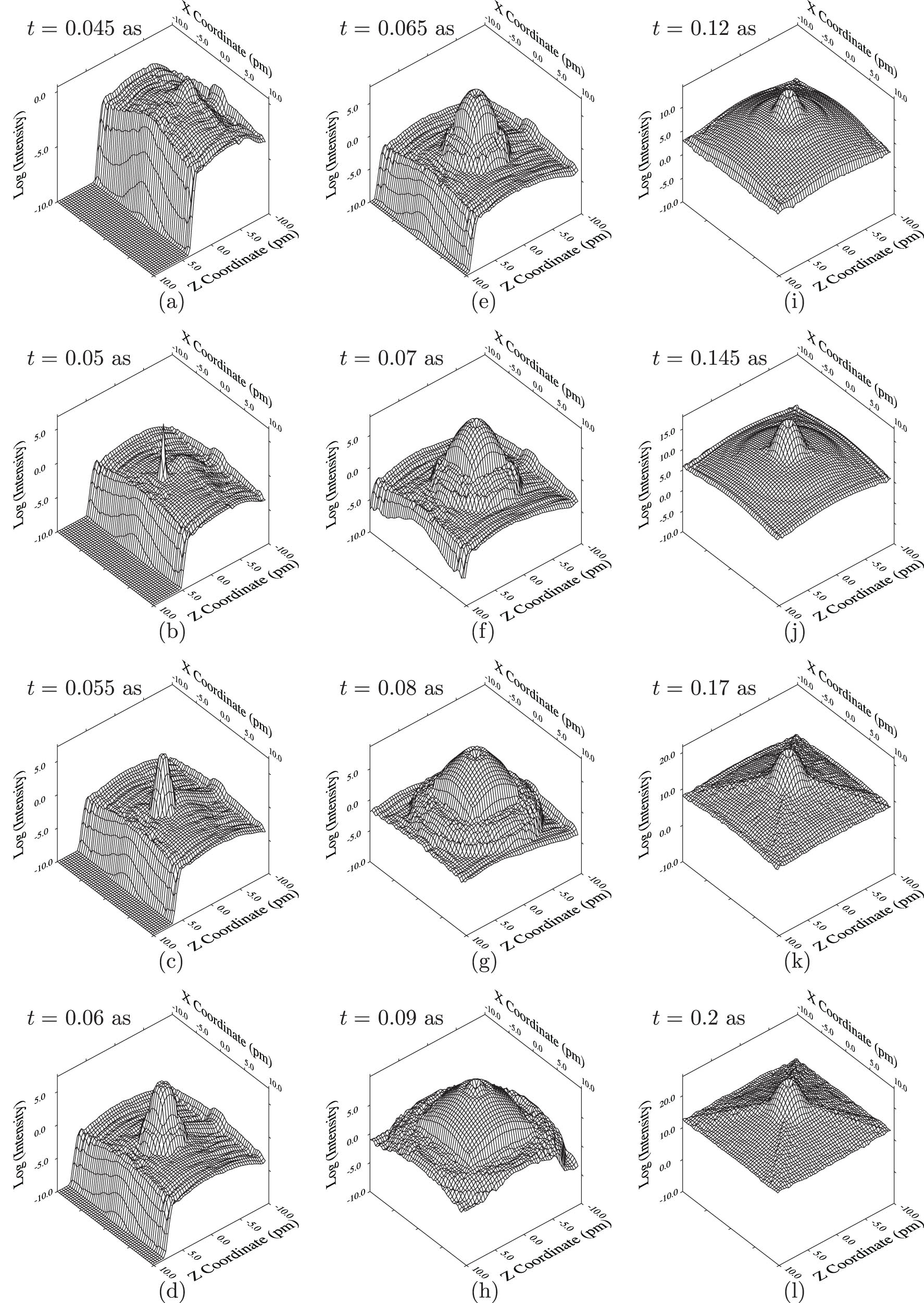
Time dependence of the eight-element Dirac field intensity in the potential of

Final orbital radius dependence on
5 Conclusion
The transient analysis of the Dirac fields has been successfully implemented using the FDTD method based on the eight-element Dirac equation, which includes dual four-element wave functions and five spatially symmetric 8
-
Funding information: The author states no funding involved.
-
Author contributions: The author has accepted responsibility for the entire content of this manuscript and approved its submission.
-
Conflict of interest: The author states no conflict of interest.
References
[1] Ohno K, Mutoh H, Harada Y. Application of Penning ionization electron spectroscopy to the study of chemical reactions on the solid surface; Photooxidation of naphthacene and rubrene. Surface Sci. 1982;115(3):L128–32. 10.1016/0039-6028(82)90373-9Search in Google Scholar
[2] Ohno K, Fujisawa S, Mutoh H, Harada Y. Application of Penning ionization electron spectroscopy to stereochemistry. Steric shielding effect of methyl groups on Penning ionization in substituted anilines. J Phys Chem. 1982;86(4):440–1. 10.1021/j100393a004Search in Google Scholar
[3] Ohno K, Mutoh H, Harada Y. Study of electron distributions of molecular orbitals by Penning ionization electron spectroscopy. J Am Chem Soc. 1983;105(14):4555–61. 10.1021/ja00352a009Search in Google Scholar
[4] Harada Y, Ohno K, Mutoh H. Penning ionization electron spectroscopy of CO and Fe (CO) 5. Study of electronic structure of Fe (CO) 5 from electron distribution of individual molecular orbitals. J Chem Phys. 1983;79:3251. 10.1063/1.446218Search in Google Scholar
[5] Veszprémi T, Harada Y, Ohno K, Mutoh H. Photoelectron and Penning ionization electron spectroscopic investigation of trimethylsilyl- and t-butyl-thiophenes. J Organometallic Chem. 1983;252(2):121–5. 10.1016/0022-328X(83)80074-6Search in Google Scholar
[6] Veszprémi T, Harada Y, Ohno K, Mutoh H. Photoelectron and Penning ionization electron spectroscopic investigation of trimethylphenylsilane. J Organometallic Chem. 1983;244(2):115–8. 10.1016/S0022-328X(00)98590-5Search in Google Scholar
[7] Veszprémi T, Harada Y, Ohno K, Mutoh H. Photoelectron and Penning electron spectroscopic investigation of phenylhalosilanes. J Organometallic Chem. 1984;266(1):9–16. 10.1016/0022-328X(84)80104-7Search in Google Scholar
[8] Veszprémi T, Harada Y, Ohno K, Mutoh H. Photoelectron and Penning ionization electron spectroscopic investigation of some silazanes. J Organometallic Chem. 1985;280(1):39–43. 10.1016/0022-328X(85)87060-1Search in Google Scholar
[9] Mutoh H, Masuda S. Spatial distribution of valence electrons in metallocenes studied by Penning ionization electron spectroscopy. J Chem Soc. Dalton Trans. 2002;9:1875–81. 10.1039/b111486gSearch in Google Scholar
[10] Yamazaki M, Horio T, Kishimoto N, Ohno K. Determination of outer molecular orbitals by collisional ionization experiments and comparison with Hartree-Fock, Kohn-Sham, and Dyson orbitals. Phys Rev A. 2007;75:032721. 10.1103/PhysRevA.75.032721Search in Google Scholar
[11] Eland JHD. Photoelectron spectroscopy. 2nd ed. London: Butterworth; 1984. 10.1016/B978-0-408-71057-2.50005-3Search in Google Scholar
[12] Paul PM, Toma ES, Breger P, Mullot G, Agostini P. Observation of a train of attosecond pulses from high harmonic generation. Science. 2001;292:1689. 10.1126/science.1059413Search in Google Scholar PubMed
[13] Itatani J, Levesque J, Zeidler D, Niikura H, Pepin H, Kieffer JC, et al. Tomographic imaging of molecular orbitals. Nature. 2004;432:867–71. 10.1038/nature03183Search in Google Scholar PubMed
[14] Yagishita A, Hosaka K, Adachi J. Photoelectron angular distributions from fixed-in-space molecules. J Electron Spectrosc Relat Phenom. 2005;142:295–312. 10.1016/j.elspec.2004.09.005Search in Google Scholar
[15] Niikura H, Wörner HJ, Villeneuve DM, Corkum PB. Probing the spatial structure of a molecular attosecond electron wave packet using shaped recollision trajectories. Phys Rev Lett. 2011;107:093004. 10.1103/PhysRevLett.107.093004Search in Google Scholar PubMed
[16] Weigold E, Hood ST, Teubner PJO. Energy and angular correlations of the scattered and ejected electrons in the electron-impact ionization of argon. Phys Rev Lett. 1973;30:475–8. 10.1103/PhysRevLett.30.475Search in Google Scholar
[17] McCarthy IE, Weigold E. (e, 2e) spectroscopy. Phys Rep. 1976;27:275–371. 10.1016/0370-1573(76)90005-3Search in Google Scholar
[18] Brion CE. Looking at orbitals in the laboratory: the experimental investigation of molecular wavefunctions and binding energies by electron momentum spectroscopy. Int J Quant Chem. 1986;29:1397–428. 10.1002/qua.560290534Search in Google Scholar
[19] McCarthy IE, Weigold E. Electron momentum spectroscopy of atoms and molecules. Rep Prog Phys. 1991;54:789–879. 10.1088/0034-4885/54/6/001Search in Google Scholar
[20] Coplan MA, Moore JH, Doering JP. (e, 2e) spectroscopy. Rev Mod Phys. 1994;66:985–1014. 10.1103/RevModPhys.66.985Search in Google Scholar
[21] Yamazaki M, Oishi K, Nakazawa H, Zhu C, Takahashi M. Molecular orbital imaging of the acetone S 2 excited state using time-resolved (e, 2e) electron momentum spectroscopy. Phys Rev Lett. 2015;114:103005. 10.1364/UP.2016.UTh4A.4Search in Google Scholar
[22] Mulliken RS. The assignment of quantum numbers for electrons in molecules II. Phys Rev. 1928;32:761. 10.1103/PhysRev.32.761Search in Google Scholar
[23] Hückel E. Quantum theory of double linkings. Z Phys. 1930;60:423. 10.1007/BF01341254Search in Google Scholar
[24] Hartree DR. The wave mechanics of an atom with a non-Coulomb central field. Part I. Theory and methods. Proc Camb Phil Soc. 1928;24:89. 10.1017/S0305004100011919Search in Google Scholar
[25] Fock V. Näherungsmethode zur Lösung des quantenmechanischen Mehrkörperproblems. Z Phys. 1930;61:126. 10.1007/BF01340294Search in Google Scholar
[26] Slater JC. Atomic shielding constants. Phys Rev. 1930;36:57. 10.1103/PhysRev.36.57Search in Google Scholar
[27] Hoffman R. An extended Hückel theory. I. Hydrocarbons. J Chem Phys. 1963;39:1397. 10.1063/1.1734456Search in Google Scholar
[28] Pople JA, Segal GA. Approximate self-consistent molecular orbital theory. III. CNDO results for AB2 and AB3 systems. J Chem Phys. 1966;44:3289. 10.1063/1.1727227Search in Google Scholar
[29] Roothaan CCJ. Self-consistent field theory for open shells of electronic systems. Rev Mod Phys. 1960;32:179. 10.1103/RevModPhys.32.179Search in Google Scholar
[30] Hay PJ. Gaussian basis sets for molecular calculations. The representation of 3d orbitals in transition‐metal atoms. J Chem Phys. 1977;66:4377. 10.1063/1.433731Search in Google Scholar
[31] Yee KS. Numerical solution of initial boundary value problems involving Maxwell’s equations in isotropic media. IEEE Trans Antennas Propagat. 1966;14:302. 10.1109/TAP.1966.1138693Search in Google Scholar
[32] Taflove A, Hagness SC. Computational electrodynamics: the finite-difference time-domain method. third edition. Norwood, MA: Artech House; 1995. Search in Google Scholar
[33] Simicevic N. Three-dimensional finite difference-time domain solution of Dirac equation. 2008. arXiv:physics.comp-ph:0812.1807v1. Search in Google Scholar
[34] Simicevic N. Finite difference-time domain solution of Dirac equation and the Klein paradox. 2009. arXiv:quant-ph:0901.3765v1. Search in Google Scholar
[35] Mutoh H. Extension of Maxwell’s equations for charge creation-annihilation and its applications. In: Proceedings on 2018 Progress in Electromagnetics Research Symposium. 2018. p. 2537–45. 10.23919/PIERS.2018.8597609Search in Google Scholar
[36] Mutoh H. Extended Maxwell’s Diamond equations to unify electromagnetism, weak gravitation, and classical and quantum mechanics and their applications for semiconductor devices. In: Proceedings on 2019 Progress in Electromagnetics Research Symposium. 2019. p. 1749–56. 10.1109/PIERS-Spring46901.2019.9017460Search in Google Scholar
[37] Dirac PAM. The principles of quantum mechanics, 4th edition. Oxford: Oxford University Press; 1958. Search in Google Scholar
[38] Peskin ME, Schroeder DV. An introduction to quantum field theory. Boulder, Colorad: Westview; 1995. Search in Google Scholar
[39] Mandl F, Shaw G. Quantum field theory. 2nd edition. Chichester, West Sussex, UK: Wiley; 2010. Search in Google Scholar
[40] Sakurai JJ. Modern quantum mechanics. 2nd edition. San Francisco, CA: Addison-Wesley; 2011. Search in Google Scholar
[41] Schrödinger E. Zur Quantendynamik des Elektrons. Sitzungsberichte der Preußischen Akademie der Wissenschaften. Physikalisch-mathematische Klasse. In: Proceedings of the Prussian Academy of Sciences, Physical-mathematical class. Berlin: Deutsche Akademie der Wissenschaften (German Academy of Sciences); 1931. p. 63–72. Search in Google Scholar
[42] Sakurai JJ. Advanced quantum mechanics. San Francisco, CA: Addison-Wesley; 1967. Search in Google Scholar
[43] Schiff LI. Quantum mechanics. 3rd edition. New York: McGraw-Hill; 1970. Search in Google Scholar
© 2023 the author(s), published by De Gruyter
This work is licensed under the Creative Commons Attribution 4.0 International License.
Articles in the same Issue
- Regular Articles
- Dynamic properties of the attachment oscillator arising in the nanophysics
- Parametric simulation of stagnation point flow of motile microorganism hybrid nanofluid across a circular cylinder with sinusoidal radius
- Fractal-fractional advection–diffusion–reaction equations by Ritz approximation approach
- Behaviour and onset of low-dimensional chaos with a periodically varying loss in single-mode homogeneously broadened laser
- Ammonia gas-sensing behavior of uniform nanostructured PPy film prepared by simple-straightforward in situ chemical vapor oxidation
- Analysis of the working mechanism and detection sensitivity of a flash detector
- Flat and bent branes with inner structure in two-field mimetic gravity
- Heat transfer analysis of the MHD stagnation-point flow of third-grade fluid over a porous sheet with thermal radiation effect: An algorithmic approach
- Weighted survival functional entropy and its properties
- Bioconvection effect in the Carreau nanofluid with Cattaneo–Christov heat flux using stagnation point flow in the entropy generation: Micromachines level study
- Study on the impulse mechanism of optical films formed by laser plasma shock waves
- Analysis of sweeping jet and film composite cooling using the decoupled model
- Research on the influence of trapezoidal magnetization of bonded magnetic ring on cogging torque
- Tripartite entanglement and entanglement transfer in a hybrid cavity magnomechanical system
- Compounded Bell-G class of statistical models with applications to COVID-19 and actuarial data
- Degradation of Vibrio cholerae from drinking water by the underwater capillary discharge
- Multiple Lie symmetry solutions for effects of viscous on magnetohydrodynamic flow and heat transfer in non-Newtonian thin film
- Thermal characterization of heat source (sink) on hybridized (Cu–Ag/EG) nanofluid flow via solid stretchable sheet
- Optimizing condition monitoring of ball bearings: An integrated approach using decision tree and extreme learning machine for effective decision-making
- Study on the inter-porosity transfer rate and producing degree of matrix in fractured-porous gas reservoirs
- Interstellar radiation as a Maxwell field: Improved numerical scheme and application to the spectral energy density
- Numerical study of hybridized Williamson nanofluid flow with TC4 and Nichrome over an extending surface
- Controlling the physical field using the shape function technique
- Significance of heat and mass transport in peristaltic flow of Jeffrey material subject to chemical reaction and radiation phenomenon through a tapered channel
- Complex dynamics of a sub-quadratic Lorenz-like system
- Stability control in a helicoidal spin–orbit-coupled open Bose–Bose mixture
- Research on WPD and DBSCAN-L-ISOMAP for circuit fault feature extraction
- Simulation for formation process of atomic orbitals by the finite difference time domain method based on the eight-element Dirac equation
- A modified power-law model: Properties, estimation, and applications
- Bayesian and non-Bayesian estimation of dynamic cumulative residual Tsallis entropy for moment exponential distribution under progressive censored type II
- Computational analysis and biomechanical study of Oldroyd-B fluid with homogeneous and heterogeneous reactions through a vertical non-uniform channel
- Predictability of machine learning framework in cross-section data
- Chaotic characteristics and mixing performance of pseudoplastic fluids in a stirred tank
- Isomorphic shut form valuation for quantum field theory and biological population models
- Vibration sensitivity minimization of an ultra-stable optical reference cavity based on orthogonal experimental design
- Effect of dysprosium on the radiation-shielding features of SiO2–PbO–B2O3 glasses
- Asymptotic formulations of anti-plane problems in pre-stressed compressible elastic laminates
- A study on soliton, lump solutions to a generalized (3+1)-dimensional Hirota--Satsuma--Ito equation
- Tangential electrostatic field at metal surfaces
- Bioconvective gyrotactic microorganisms in third-grade nanofluid flow over a Riga surface with stratification: An approach to entropy minimization
- Infrared spectroscopy for ageing assessment of insulating oils via dielectric loss factor and interfacial tension
- Influence of cationic surfactants on the growth of gypsum crystals
- Study on instability mechanism of KCl/PHPA drilling waste fluid
- Analytical solutions of the extended Kadomtsev–Petviashvili equation in nonlinear media
- A novel compact highly sensitive non-invasive microwave antenna sensor for blood glucose monitoring
- Inspection of Couette and pressure-driven Poiseuille entropy-optimized dissipated flow in a suction/injection horizontal channel: Analytical solutions
- Conserved vectors and solutions of the two-dimensional potential KP equation
- The reciprocal linear effect, a new optical effect of the Sagnac type
- Optimal interatomic potentials using modified method of least squares: Optimal form of interatomic potentials
- The soliton solutions for stochastic Calogero–Bogoyavlenskii Schiff equation in plasma physics/fluid mechanics
- Research on absolute ranging technology of resampling phase comparison method based on FMCW
- Analysis of Cu and Zn contents in aluminum alloys by femtosecond laser-ablation spark-induced breakdown spectroscopy
- Nonsequential double ionization channels control of CO2 molecules with counter-rotating two-color circularly polarized laser field by laser wavelength
- Fractional-order modeling: Analysis of foam drainage and Fisher's equations
- Thermo-solutal Marangoni convective Darcy-Forchheimer bio-hybrid nanofluid flow over a permeable disk with activation energy: Analysis of interfacial nanolayer thickness
- Investigation on topology-optimized compressor piston by metal additive manufacturing technique: Analytical and numeric computational modeling using finite element analysis in ANSYS
- Breast cancer segmentation using a hybrid AttendSeg architecture combined with a gravitational clustering optimization algorithm using mathematical modelling
- On the localized and periodic solutions to the time-fractional Klein-Gordan equations: Optimal additive function method and new iterative method
- 3D thin-film nanofluid flow with heat transfer on an inclined disc by using HWCM
- Numerical study of static pressure on the sonochemistry characteristics of the gas bubble under acoustic excitation
- Optimal auxiliary function method for analyzing nonlinear system of coupled Schrödinger–KdV equation with Caputo operator
- Analysis of magnetized micropolar fluid subjected to generalized heat-mass transfer theories
- Does the Mott problem extend to Geiger counters?
- Stability analysis, phase plane analysis, and isolated soliton solution to the LGH equation in mathematical physics
- Effects of Joule heating and reaction mechanisms on couple stress fluid flow with peristalsis in the presence of a porous material through an inclined channel
- Bayesian and E-Bayesian estimation based on constant-stress partially accelerated life testing for inverted Topp–Leone distribution
- Dynamical and physical characteristics of soliton solutions to the (2+1)-dimensional Konopelchenko–Dubrovsky system
- Study of fractional variable order COVID-19 environmental transformation model
- Sisko nanofluid flow through exponential stretching sheet with swimming of motile gyrotactic microorganisms: An application to nanoengineering
- Influence of the regularization scheme in the QCD phase diagram in the PNJL model
- Fixed-point theory and numerical analysis of an epidemic model with fractional calculus: Exploring dynamical behavior
- Computational analysis of reconstructing current and sag of three-phase overhead line based on the TMR sensor array
- Investigation of tripled sine-Gordon equation: Localized modes in multi-stacked long Josephson junctions
- High-sensitivity on-chip temperature sensor based on cascaded microring resonators
- Pathological study on uncertain numbers and proposed solutions for discrete fuzzy fractional order calculus
- Bifurcation, chaotic behavior, and traveling wave solution of stochastic coupled Konno–Oono equation with multiplicative noise in the Stratonovich sense
- Thermal radiation and heat generation on three-dimensional Casson fluid motion via porous stretching surface with variable thermal conductivity
- Numerical simulation and analysis of Airy's-type equation
- A homotopy perturbation method with Elzaki transformation for solving the fractional Biswas–Milovic model
- Heat transfer performance of magnetohydrodynamic multiphase nanofluid flow of Cu–Al2O3/H2O over a stretching cylinder
- ΛCDM and the principle of equivalence
- Axisymmetric stagnation-point flow of non-Newtonian nanomaterial and heat transport over a lubricated surface: Hybrid homotopy analysis method simulations
- HAM simulation for bioconvective magnetohydrodynamic flow of Walters-B fluid containing nanoparticles and microorganisms past a stretching sheet with velocity slip and convective conditions
- Coupled heat and mass transfer mathematical study for lubricated non-Newtonian nanomaterial conveying oblique stagnation point flow: A comparison of viscous and viscoelastic nanofluid model
- Power Topp–Leone exponential negative family of distributions with numerical illustrations to engineering and biological data
- Extracting solitary solutions of the nonlinear Kaup–Kupershmidt (KK) equation by analytical method
- A case study on the environmental and economic impact of photovoltaic systems in wastewater treatment plants
- Application of IoT network for marine wildlife surveillance
- Non-similar modeling and numerical simulations of microploar hybrid nanofluid adjacent to isothermal sphere
- Joint optimization of two-dimensional warranty period and maintenance strategy considering availability and cost constraints
- Numerical investigation of the flow characteristics involving dissipation and slip effects in a convectively nanofluid within a porous medium
- Spectral uncertainty analysis of grassland and its camouflage materials based on land-based hyperspectral images
- Application of low-altitude wind shear recognition algorithm and laser wind radar in aviation meteorological services
- Investigation of different structures of screw extruders on the flow in direct ink writing SiC slurry based on LBM
- Harmonic current suppression method of virtual DC motor based on fuzzy sliding mode
- Micropolar flow and heat transfer within a permeable channel using the successive linearization method
- Different lump k-soliton solutions to (2+1)-dimensional KdV system using Hirota binary Bell polynomials
- Investigation of nanomaterials in flow of non-Newtonian liquid toward a stretchable surface
- Weak beat frequency extraction method for photon Doppler signal with low signal-to-noise ratio
- Electrokinetic energy conversion of nanofluids in porous microtubes with Green’s function
- Examining the role of activation energy and convective boundary conditions in nanofluid behavior of Couette-Poiseuille flow
- Review Article
- Effects of stretching on phase transformation of PVDF and its copolymers: A review
- Special Issue on Transport phenomena and thermal analysis in micro/nano-scale structure surfaces - Part IV
- Prediction and monitoring model for farmland environmental system using soil sensor and neural network algorithm
- Special Issue on Advanced Topics on the Modelling and Assessment of Complicated Physical Phenomena - Part III
- Some standard and nonstandard finite difference schemes for a reaction–diffusion–chemotaxis model
- Special Issue on Advanced Energy Materials - Part II
- Rapid productivity prediction method for frac hits affected wells based on gas reservoir numerical simulation and probability method
- Special Issue on Novel Numerical and Analytical Techniques for Fractional Nonlinear Schrodinger Type - Part III
- Adomian decomposition method for solution of fourteenth order boundary value problems
- New soliton solutions of modified (3+1)-D Wazwaz–Benjamin–Bona–Mahony and (2+1)-D cubic Klein–Gordon equations using first integral method
- On traveling wave solutions to Manakov model with variable coefficients
- Rational approximation for solving Fredholm integro-differential equations by new algorithm
- Special Issue on Predicting pattern alterations in nature - Part I
- Modeling the monkeypox infection using the Mittag–Leffler kernel
- Spectral analysis of variable-order multi-terms fractional differential equations
- Special Issue on Nanomaterial utilization and structural optimization - Part I
- Heat treatment and tensile test of 3D-printed parts manufactured at different build orientations