Flat and bent branes with inner structure in two-field mimetic gravity
-
Qian Xiang


Abstract
Inspired by the work Zhong et al. (2018), we study the linear tensor perturbation of both the flat and bent thick branes with inner structure in two-field mimetic gravity. The master equations for the linear tensor perturbations are derived by taking the transverse and traceless gauges. For the Minkowski and Anti-de-Sitter brane, the brane systems are stable against the tensor perturbation. The effective potentials of the tensor perturbations of both the flat and bent thick branes are volcano-like, and this structure may potentially lead to the zero-mode and the resonant modes of the tensor perturbation. We further illustrate the results of massive resonant modes.
1 Introduction
The braneworld theory has received much attention over the past years since it proposes a new route to possibly solve the gauge hierarchy problem and the cosmological constant problem [1–4]. The Randall–Sundrum (RS) models [3,4] are typical examples of them with a non-factorizable metric and a warped extra dimension. It is shown that RS models give rise to thin brane profiles because the warp factor has cusp singularities at the brane positions. Several proposals for generalizing thin branes into thick branes have been presented in the literature. The thick branes are obtained by introducing one or more bulk scalar fields coupled to gravity [5–15] or realized by pure geometric frameworks without background matter fields considered in refs [16–19]. Most of the models study Minkowski branes, and a few of them consider the curvature of the embedded brane, which includes de Sitter (
On the other hand, mimetic gravity is proposed by Chamseddine and Mukhanov [20] as one of the extensions of general relativity (GR). In the original setup, a physical metric
As we know, the scalar fields are usually introduced to generate the topological defects, such as kinks and domain walls, for realizing the thick branes, so it is natural to generate the domain walls by the mimetic scalar fields. However, suffering from the ghost and gradient instabilities, the original mimetic theory with a single field could not suffice [54]. For the single-field mimetic scenario, one can go to a ghost-free theory by adding higher derivative terms to the original theory [55]. For the two-field extension of the mimetic gravity put forward in ref. [56], the double scalar fields version not only avoids the above problem but also allows us to construct the thick branes with a complicated inner structure. It is common to find the background solution of the thick branes via the first-order formalism [11] or the extension method [57]. However, in the two-field mimetic theory, the gravity and two mimetic scalars are coupled. It is relatively harder to find the domain wall solutions if the four-dimensional geometry is either flat or curved. In this work, we apply the reconstruction technique [58] to seek the background solutions of three cases of thick branes. The approach gives the form of the warp factor and scalar fields, and provides a direct way to investigate the other variables. We consider that the thick domain walls possess four-dimensional
This article is organized as follows. In Section 2, we introduce the mimetic thick brane model and consider three cases of thick branes. In Section 3, we analyze the stability of the model under the linear tensor perturbation and study the localization of gravity zero-mode. Finally, a brief conclusion is presented in Section 5. Throughout this article, capital Latin letters
2 Brane setup and field equations
We consider the five-dimensional, two-field mimetic gravity where the action is the Einstein–Hilbert action constructed in terms of the physical metric
where the Lagrangian of the two interacting mimetic scalar fields is generalized as follows:
In the original mimetic model,
The variation of the action (1) concerning the metric
The line-element for a warped five-dimensional geometry is generally assumed as follows:
with
where
We know that Eqs. (3) and (4) determine the solution of the brane system. There are three independent equations and six variables in this system. To solve this system, we should preset three variables. Based on the reconstruction technique, we will give the form of
where

Plots of the warp factor
2.1 Flat brane
For Minkowski brane, we take
Eqs. (4) and (3) can be reduced to
where the prime denotes the derivative with respect to
2.2 Bent branes
We now turn attention to the case of
Eqs. (4) and (3) can be reduced to
Now the system can be solved as follows:
For AdS case (
So far, we have obtained the background solution of the three cases of thick branes. In more detail, the potential
we can obtain the dimensionless quantities. The profiles of the potential

The potential

Comparison of the dimensionless scalar potential
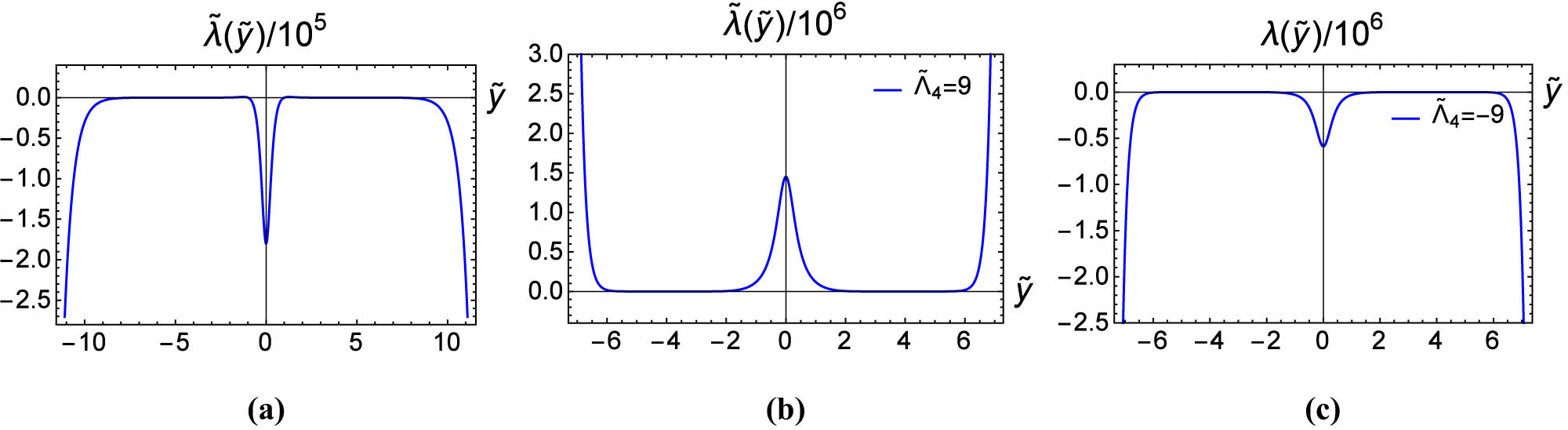
Comparison of Lagrange multiplier
3 Linear tensor perturbation
In the case of the tensor perturbation, we suppose that the space-time undergoes a small perturbation
where
with the first-order perturbed metric as
where
3.1 Flat brane
For the tensor perturbation of flat brane, the perturbed metric is given as follows:
where
where
Under the TT condition, the perturbation of the
where the four-dimensional d’Alembertian is defined as
By imposing a coordinate transformation,
Considering the Kaluza–Klein (KK) decomposition
where
This equation can be factorized as
and this structure ensures that the eigenvalues are non-negative, which means that the brane is stable against the tensor perturbation. Since the potential vanishes for large
To localize the gravity zero-mode,
which is finite when

The influence of
3.2 Bent branes
We now turn to the case of
where the four-dimensional metric is decomposed into a small perturbation
The interesting investigations of the tensor perturbation have already appeared in refs. [7,61] and in references therein. Then, under the TT gauge condition
where
Here,
for
At the boundaries of the brane, the potential
which ensures the stability of the tensor perturbation.
4 Massive resonant modes
For the volcano-like effective potentials, the tensor perturbation has zero-mode and may also have resonant modes. Resonant frequencies A further investigation of the metastable modes is necessary. Because the integral
To find the massive resonant states, we use the numerical method given in refs [62–65], where a relative probability was proposed as follows:
Here,
4.1 Flat brane
When the wave functions are either even-parity or odd-parity, the Schrödinger-like equation can be solved numerically. The dimensionless effective potential

The influence of parameter
From Figure 6, we see that, with the increasing of the parameter

The wave functions for the first even- and odd-parity modes for the flat brane (
The influence of the parameter
|
|
|
|
Parity |
|
|
|
|
|---|---|---|---|---|---|---|---|
| 3 | 0 | 1 | Even | 0.1988 | 0.372419 | 0.00810986 | 123.307 |
| 0 | 2 | Odd | 1.8477 | 0.144147 | 1.15022 | 0.8694 | |
| 8 | 0 | 1 | Odd | 0.0176 | 0.644363 | 0.00112908 | 885.681 |
| 0 | 2 | Even | 0.0177 | 0.336324 | 0.00112589 | 888.186 | |
| 0 | 3 | Odd | 0.0419 | 0.923572 | 0.000732362 | 1365.44 | |
| 0 | 4 | Even | 0.0424 | 0.850191 | 0.000727779 | 1374.04 | |
| 0 | 5 | Odd | 0.0763 | 0.933456 | 0.000905549 | 1104.30 | |
| 0 | 6 | Even | 0.0779 | 0.94479 |
|
1116.43 | |
| 0 | 7 | Odd | 0.1205 | 0.909459 | 0.00172875 | 578.454 | |
| 0 | 8 | Even | 0.1241 | 0.89555 | 0.00141991 | 587.129 | |
| 0 | 9 | Odd | 0.1745 | 0.792877 | 0.00215697 | 278.884 | |
| 0 | 10 | Even | 0.1808 | 0.755761 | 0.00358572 | 404.900 |
4.2 Bent branes
Because the tensor perturbation of
The effects of the parameters

The influence of the parameter
The influence of the parameter
|
|
|
|
||||||
|---|---|---|---|---|---|---|---|---|
|
|
|
|
|
|
|
|
|
|
| 0.1988 | 0.047 | 0.0176 | 18.1988 | 18.047 | 18.0176 | 27.1988 | 27.047 | 27.0176 |
| 1.8477 | 0.0481 | 0.0177 | 19.8477 | 18.0481 | 18.0177 | 28.8477 | 27.0481 | 27.0177 |
| — | 0.1104 | 0.0419 | — | 18.1104 | 18.0419 | — | 27.1104 | 27.0419 |
| — | 0.1156 | 0.0424 | — | 18.1156 | 18.0424 | — | 27.1156 | 27.0424 |
| — | 0.199 | 0.0763 | — | 18.199 | 18.0763 | — | 27.199 | 27.0763 |
| — | 0.2122 | 0.0779 | — | 18.2122 | 18.0779 | — | 27.2122 | 27.0779 |
| — | 0.3123 | 0.1205 | — | 18.3123 | 18.1205 | — | 27.3123 | 27.1205 |
| — | 0.3375 | 0.1241 | — | 18.3375 | 18.1241 | — | 27.3375 | 27.1241 |
| — | — | 0.1745 | — | — | 18.1745 | — | — | 27.1745 |
| — | — | 0.1808 | — | — | 18.1808 | — | — | 27.1808 |
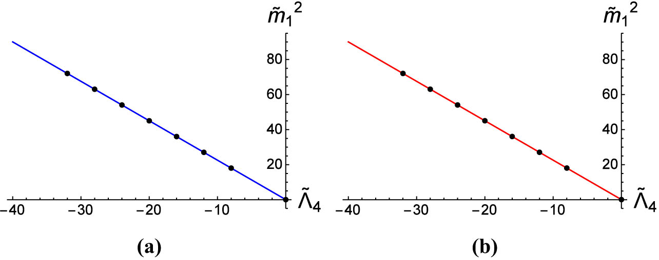
We plot the fit functions for masses of the first even-parity and odd-parity modes with different
The influence of

The wave functions for the first even-parity and first odd-parity modes with
For
The influence of the parameter
|
|
|
|
Parity |
|
|
|
|
|---|---|---|---|---|---|---|---|
| 3 |
|
1 | Even | 18.1988 | 0.372419 | 0.00810986 | 123.307 |
|
|
2 | Odd | 19.8477 | 0.144147 | 1.15022 | 0.8694 | |
| 8 |
|
1 | Odd | 18.0176 | 0.644363 | 0.00112908 | 885.681 |
|
|
2 | Even | 18.0177 | 0.336324 | 0.00112589 | 888.186 | |
|
|
3 | Odd | 18.0419 | 0.923572 | 0.000732362 | 1365.44 | |
|
|
4 | Even | 18.0424 | 0.850191 | 0.000727779 | 1374.04 | |
|
|
5 | Odd | 18.0763 | 0.933456 | 0.000905549 | 1104.30 | |
|
|
6 | Even | 18.0779 | 0.94479 | 0.00089571 | 1116.43 | |
|
|
7 | Odd | 18.1205 | 0.909459 | 0.00172875 | 578.454 | |
|
|
8 | Even | 18.1241 | 0.89555 | 0.00141991 | 587.129 | |
|
|
9 | Odd | 18.1745 | 0.792877 | 0.00215697 | 278.884 | |
|
|
10 | Even | 18.1808 | 0.755761 | 0.00358572 | 404.900 |
5 Conclusion
In this article, we investigate the linear tensor perturbation for
When
As the parameter
Moreover, we would like to point out that the tensor perturbation of the two-field mimetic gravity model is the same as that of the original single-field mimetic theory [52] and GR. Nevertheless, the two mimetic scalar fields can generate different thick branes, leading to new types of effective potential and graviton resonant modes. There are some interesting extensions of this work. The resonant frequencies and spectroscopy of black holes are analyzed in refs [66,67]. The frequencies of resonant mode in braneworld are not discussed in this article, which will be left to our further study.
Acknowledgments
The authors sincerely thank Prof. Yu-Xiao Liu for the helpful discussions.
-
Funding information: This work is supported by the National Key Research and Development Program of China (Grant No. 2020YFC2201503) and the National Natural Science Foundation of China (Grant No. 12247101). Yi Zhong was supported by the Fundamental Research Funds for the Central Universities (Grant No. 531118010195).
-
Author contributions: All authors have accepted responsibility for the entire content of this manuscript and approved its submission.
-
Conflict of interest: The authors state no conflict of interest.
References
[1] Arkani-Hamed N, Dimopoulos S, Dvali GR. The hierarchy problem and new dimensions at a millimeter. Phys Lett B. 1998;429:263–72. 10.1016/S0370-2693(98)00466-3Search in Google Scholar
[2] Antoniadis I, Arkani-Hamed N, Dimopoulos S, Dvali GR. New dimensions at a millimeter to a fermi and superstrings at a TeV. Phys Lett B. 1998;436:257–63. 10.1016/S0370-2693(98)00860-0Search in Google Scholar
[3] Randall L, Sundrum R. Large mass hierarchy from a small extra dimension. Phys Rev Lett. 1999;83:3370–3. 10.1103/PhysRevLett.83.3370Search in Google Scholar
[4] Randall L, Sundrum R. An alternative to compactification. Phys Rev Lett. 1999;83:4690–3. 10.1103/PhysRevLett.83.4690Search in Google Scholar
[5] Gremm M. Four-dimensional gravity on a thick domain wall. Phys Lett B. 2000;478:434–8. 10.1016/S0370-2693(00)00303-8Search in Google Scholar
[6] DeWolfe O, Freedman DZ, Gubser SS, Karch A. Modeling the fifth dimension with scalars and gravity. Phys Rev D. 2000;62:046008. 10.1103/PhysRevD.62.046008Search in Google Scholar
[7] Kobayashi S, Koyama K, Soda J. Thick brane worlds and their stability. Phys Rev D. 2002;65:064014. 10.1103/PhysRevD.65.064014Search in Google Scholar
[8] Bazeia D, Losano L, Wotzasek C. Domain walls in three-field models. Phys Rev D. 2002;66:105025. 10.1103/PhysRevD.66.105025Search in Google Scholar
[9] Wang A. Thick de Sitter 3-branes, dynamic black holes, and localization of gravity. Phys Rev D. 2002;66:024024. 10.1103/PhysRevD.66.024024Search in Google Scholar
[10] Bazeia D, Gomes AR. Bloch brane. JHEP. 2004;5:012. 10.1088/1126-6708/2004/05/012Search in Google Scholar
[11] Afonso VI, Bazeia D, Losano L. First-order formalism for bent brane. Phys Lett B. 2006;634:526–30. 10.1016/j.physletb.2006.02.017Search in Google Scholar
[12] Bazeia D, Brito FA, Losano L. Scalar fields, bent branes, and RG flow. JHEP. 2006;11:064. 10.1088/1126-6708/2006/11/064Search in Google Scholar
[13] Bogdanos C, Dimitriadis A, Tamvakis K. Brane models with a Ricci-coupled scalar field. Phys Rev D. 2006;74:045003. 10.1103/PhysRevD.74.045003Search in Google Scholar
[14] Dzhunushaliev V, Folomeev V, Minamitsuji M. Thick brane solutions. Rept Prog Phys. 2010;73:066901. 10.1088/0034-4885/73/6/066901Search in Google Scholar
[15] Liu YX, Zhong Y, Yang K. Scalar-kinetic branes. EPL. 2010;90(5):51001. 10.1209/0295-5075/90/51001Search in Google Scholar
[16] Barbosa-Cendejas N, Herrera-Aguilar A. 4D gravity localized in non Bbb Z2-symmetric thick branes. JHEP. 2005;10:101. 10.1088/1126-6708/2005/10/101Search in Google Scholar
[17] Herrera-Aguilar A, Malagon-Morejon D, Mora-Luna RR. Localization of gravity on a de Sitter thick braneworld without scalar fields. JHEP. 2010;11:015. 10.1007/JHEP11(2010)015Search in Google Scholar
[18] Zhong Y, Liu YX. Pure geometric thick f(R)-branes: stability and localization of gravity. Eur Phys J C. 2016;76(6):321. 10.1140/epjc/s10052-016-4163-0Search in Google Scholar
[19] Rubakov VA, Shaposhnikov ME. Extra space-time dimensions: Towards a solution to the cosmological constant problem. Phys Lett B. 1983;125:139–43. 10.1016/0370-2693(83)91254-6Search in Google Scholar
[20] Chamseddine AH, Mukhanov V. Mimetic dark matter. JHEP. 2013;11:135. 10.1007/JHEP11(2013)135Search in Google Scholar
[21] Chamseddine AH, Mukhanov V, Vikman A. Cosmology with mimetic matter. JCAP. 2014;6:17. 10.1088/1475-7516/2014/06/017Search in Google Scholar
[22] Lim EA, Sawicki I, Vikman A. Dust of dark energy. JCAP. 2010;5:12. 10.1088/1475-7516/2010/05/012Search in Google Scholar
[23] Leon G, Saridakis EN. Dynamical behavior in mimeticF(R) gravity. JCAP. 2015;4:31. 10.1088/1475-7516/2015/04/031. Search in Google Scholar
[24] Velten HES, von Marttens RF, Zimdahl W. Aspects of the cosmological coincidence problem. Eur Phys J C. 2014;74(11):3160. 10.1140/epjc/s10052-014-3160-4. Search in Google Scholar
[25] Shimon M. Elucidation of ’Cosmic Coincidence’. arXiv:2204.02211 [astro-ph.CO]. Search in Google Scholar
[26] Babichev E, Ramazanov S. Gravitational focusing of imperfect dark matter. Phys Rev D. 2017;95(2):024025. 10.1103/PhysRevD.95.024025Search in Google Scholar
[27] Sadeghnezhad N, Nozari K. Braneworld mimetic cosmology. Phys Lett B. 2017;769:134–40. 10.1016/j.physletb.2017.03.039Search in Google Scholar
[28] Casalino A, Rinaldi M, Sebastiani L, Vagnozzi S. Mimicking dark matter and dark energy in a mimetic model compatible with GW170817. Phys Dark Univ. 2018;22:108. 10.1016/j.dark.2018.10.001Search in Google Scholar
[29] Ganz A, Bartolo N, Karmakar P, Matarrese S. Gravity in mimetic scalar-tensor theories after GW170817. JCAP. 2019;1:56. 10.1088/1475-7516/2019/01/056Search in Google Scholar
[30] Zheng Y, Shen L, Mou Y, Li M. On (in)stabilities of perturbations in mimetic models with higher derivatives. JCAP. 2017;8:040. 10.1088/1475-7516/2017/08/040Search in Google Scholar
[31] Myrzakulov R, Sebastiani L, Vagnozzi S, Zerbini S. Static spherically symmetric solutions in mimetic gravity: rotation curves and wormholes. Class Quant Grav. 2016;33(12):125005. 10.1088/0264-9381/33/12/125005Search in Google Scholar
[32] Vagnozzi S. Recovering a MOND-like acceleration law in mimetic gravity. Class Quant Grav. 2017;34(18):185006. 10.1088/1361-6382/aa838bSearch in Google Scholar
[33] Casalino A, Rinaldi M, Sebastiani L, Vagnozzi S. Alive and well: mimetic gravity and a higher-order extension in light of GW170817. Class Quant Grav. 2019;36(1):017001. 10.1088/1361-6382/aaf1fdSearch in Google Scholar
[34] Malaeb O. Hamiltonian formulation of mimetic gravity. Phys Rev D. 2015;91(10):103526. 10.1103/PhysRevD.91.103526Search in Google Scholar
[35] Chaichian M, Kluson J, Oksanen M, Tureanu A. Mimetic dark matter, ghost instability and a mimetic tensor-vector-scalar gravity. JHEP. 2014;12:102. 10.1007/JHEP12(2014)102Search in Google Scholar
[36] Takahashi K, Kobayashi T. Extended mimetic gravity: Hamiltonian analysis and gradient instabilities. JCAP. 2017;11:38. 10.1142/9789811258251_0082Search in Google Scholar
[37] Zheng Y, Zheng YL. Hamiltonian analysis of mimetic gravity with higher derivatives. JHEP. 2021;1:85. 10.1007/JHEP01(2021)085Search in Google Scholar
[38] Shen LY, Zheng YL, Li MZ. Two-field mimetic gravity revisited and Hamiltonian analysis. JCAP. 2019;12:26. 10.1088/1475-7516/2019/12/026Search in Google Scholar
[39] Nojiri S, Odintsov SD. Mimetic F(R) gravity: Inflation, dark energy and bounce. Mod Phys Lett A. 2014;29(40):145021110.1142/S0217732314502113Search in Google Scholar
[40] Nojiri S, Odintsov SD, Oikonomou VK. Viable mimetic completion of unified inflation-dark energy evolution in modified gravity. Phys Rev D. 2016;94(10):104050. 10.1103/PhysRevD.94.104050Search in Google Scholar
[41] Nojiri S, Odintsov SD, Oikonomou VK. Unimodular-mimetic cosmology. Class Quant Grav. 2016;33(12):125017. 10.1088/0264-9381/33/12/125017Search in Google Scholar
[42] Odintsov SD, Oikonomou VK. Accelerating cosmologies and the phase structure of F(R)gravity with Lagrange multiplier constraints: A mimetic approach. Phys Rev D. 2016;93(2):023517. 10.1103/PhysRevD.93.023517Search in Google Scholar
[43] Odintsov SD, Oikonomou VK. Viable mimetic F(R) gravity compatible with Planck observations. Ann Phys. 2015;363:503–14. 10.1016/j.aop.2015.10.013Search in Google Scholar
[44] Astashenok AV, Odintsov SD, Oikonomou VK. Modified Gauss-Bonnet gravity with the Lagrange multiplier constraint as mimetic theory. Class Quant Grav. 2015;32(18):185007. 10.1088/0264-9381/32/18/185007Search in Google Scholar
[45] Nojiri S, Odintsov SD, Oikonomou VK. Ghost-free F(R) gravity with Lagrange multiplier constraint. Phys Lett B. 2017;775:44–9. 10.1016/j.physletb.2017.10.045Search in Google Scholar
[46] Cognola G, Myrzakulov R, Sebastiani L, Vagnozzi S, Zerbini S. Covariant Horrrava-like and mimetic Horndeski gravity: cosmological solutions and perturbations. Class Quant Grav. 2016;33(22):22501410.1088/0264-9381/33/22/225014Search in Google Scholar
[47] Hosseinkhan N, Nozari K. Late time cosmological dynamics with a nonminimal extension of the mimetic matter scenario. Eur Phys J Plus. 2018;133(2):50. 10.1140/epjp/i2018-11876-4Search in Google Scholar
[48] Chamseddine AH, Mukhanov V, Russ TB. Mimetic Hořava gravity. Phys Lett B. 2019;798:134939. 10.1016/j.physletb.2019.134939Search in Google Scholar
[49] Momeni D, Altaibayeva A, Myrzakulov R. New modified mimetic gravity. Int J Geom Meth Mod Phys. 2014;11:1450091. 10.1142/S0219887814500911Search in Google Scholar
[50] Chamseddine AH, Mukhanov V. Ghost free mimetic massive gravity. JHEP. 2018;6:60. 10.1007/JHEP06(2018)060. Search in Google Scholar
[51] Davood Sadatian S, Sepehri A. Tachyonic braneworld mimetic cosmology. Mod Phys Lett A. 2019;34(21):195016210.1142/S0217732319501621Search in Google Scholar
[52] Zhong Y, Zhong Y, Zhang YP, Liu YX. Occurrence and genotyping of Giardia duodenalis and Cryptosporidium in pre-weaned dairy calves in central Sichuan province, China. Eur Phys J C. 2018;78(1):45. 10.1051/parasite/2018046Search in Google Scholar PubMed PubMed Central
[53] Sebastiani L, Vagnozzi S, Myrzakulov R. Mimetic gravity: a review of recent developments and applications to cosmology and astrophysics. Adv High Energy Phys. 2017;2017:3156915. 10.1155/2017/3156915Search in Google Scholar
[54] Firouzjahi H, Gorji MA, Hosseini Mansoori SA. Instabilities in mimetic matter perturbations. JCAP. 2017;7:31. 10.1088/1475-7516/2017/07/031Search in Google Scholar
[55] Gorji MA, Hosseini Mansoori SA, Firouzjahi H. Higher derivative mimetic gravity. JCAP. 2018;1:20. 10.1088/1475-7516/2018/01/020Search in Google Scholar
[56] Firouzjahi H, Gorji MA, Hosseini Mansoori SA, Karami A, Rostami T. Two-field disformal transformation and mimetic cosmology. JCAP. 2018;11:046. 10.1088/1475-7516/2018/11/046Search in Google Scholar
[57] Bazeia D, Losano L, Santos JRL. Kinklike structures in scalar field theories: From one-field to two-field models. Phys Lett A. 2013;377:1615–20. 10.1016/j.physleta.2013.04.047Search in Google Scholar
[58] Higuchi M, Nojiri S. Reconstruction of domain wall universe and localization of gravity. Gen Rel Grav. 2014;46(11):1822. 10.1007/s10714-014-1822-zSearch in Google Scholar
[59] Liu YX, Yang K, Zhong Y. de Sitter thick brane solution in Weyl geometry. JHEP. 2010;10:69. 10.1007/JHEP10(2010)069Search in Google Scholar
[60] Liu YX, Guo H, Fu CE, Li HT. Localization of gravity and bulk matters on a thick anti-de Sitter brane. Phys Rev D. 2011;84:044033. 10.1103/PhysRevD.84.044033Search in Google Scholar
[61] Karch A, Randall L. Locally localized gravity. JHEP. 2001;5:8. 10.1088/1126-6708/2001/05/008Search in Google Scholar
[62] Liu YX, Fu CE, Zhao L, Duan YS. Localization and mass spectra of fermions on symmetric and asymmetric thick branes. Phys Rev D. 2009;80:065020. 10.1103/PhysRevD.80.065020Search in Google Scholar
[63] Liu YX, Yang J, Zhao ZH, Fu CE, Duan YS. Fermion localization and resonances on a de Sitter thick brane. Phys Rev D. 2009;80:065019. 10.1103/PhysRevD.80.065019Search in Google Scholar
[64] Du YZ, Zhao L, Zhong Y, Fu CE, Guo H. Resonances of Kalb–Ramond field on symmetric and asymmetric thick branes. Phys Rev D. 2013;88:024009. 10.1103/PhysRevD.88.024009Search in Google Scholar
[65] Tan Q, Guo WD, Zhang YP, Liu YX. Gravitational resonances on f(T)-branes. Eur Phys J C. 2021;81(4):373. 10.1140/epjc/s10052-021-09162-0Search in Google Scholar
[66] Vieira HS, Bezerra VB. Resonant frequencies of a massless scalar field in the canonical acoustic black hole spacetime. Gen Rel Grav. 2020;52(8):72. 10.1007/s10714-020-02726-7Search in Google Scholar
[67] Sakalli I, Tokgoz G. Spectroscopy of rotating linear dilaton black holes from boxed quasinormal modes: spectroscopy of rotating linear dilaton black holes. Annalen Phys. 2016;528:612–8. 10.1002/andp.201500305Search in Google Scholar
© 2023 the author(s), published by De Gruyter
This work is licensed under the Creative Commons Attribution 4.0 International License.
Articles in the same Issue
- Regular Articles
- Dynamic properties of the attachment oscillator arising in the nanophysics
- Parametric simulation of stagnation point flow of motile microorganism hybrid nanofluid across a circular cylinder with sinusoidal radius
- Fractal-fractional advection–diffusion–reaction equations by Ritz approximation approach
- Behaviour and onset of low-dimensional chaos with a periodically varying loss in single-mode homogeneously broadened laser
- Ammonia gas-sensing behavior of uniform nanostructured PPy film prepared by simple-straightforward in situ chemical vapor oxidation
- Analysis of the working mechanism and detection sensitivity of a flash detector
- Flat and bent branes with inner structure in two-field mimetic gravity
- Heat transfer analysis of the MHD stagnation-point flow of third-grade fluid over a porous sheet with thermal radiation effect: An algorithmic approach
- Weighted survival functional entropy and its properties
- Bioconvection effect in the Carreau nanofluid with Cattaneo–Christov heat flux using stagnation point flow in the entropy generation: Micromachines level study
- Study on the impulse mechanism of optical films formed by laser plasma shock waves
- Analysis of sweeping jet and film composite cooling using the decoupled model
- Research on the influence of trapezoidal magnetization of bonded magnetic ring on cogging torque
- Tripartite entanglement and entanglement transfer in a hybrid cavity magnomechanical system
- Compounded Bell-G class of statistical models with applications to COVID-19 and actuarial data
- Degradation of Vibrio cholerae from drinking water by the underwater capillary discharge
- Multiple Lie symmetry solutions for effects of viscous on magnetohydrodynamic flow and heat transfer in non-Newtonian thin film
- Thermal characterization of heat source (sink) on hybridized (Cu–Ag/EG) nanofluid flow via solid stretchable sheet
- Optimizing condition monitoring of ball bearings: An integrated approach using decision tree and extreme learning machine for effective decision-making
- Study on the inter-porosity transfer rate and producing degree of matrix in fractured-porous gas reservoirs
- Interstellar radiation as a Maxwell field: Improved numerical scheme and application to the spectral energy density
- Numerical study of hybridized Williamson nanofluid flow with TC4 and Nichrome over an extending surface
- Controlling the physical field using the shape function technique
- Significance of heat and mass transport in peristaltic flow of Jeffrey material subject to chemical reaction and radiation phenomenon through a tapered channel
- Complex dynamics of a sub-quadratic Lorenz-like system
- Stability control in a helicoidal spin–orbit-coupled open Bose–Bose mixture
- Research on WPD and DBSCAN-L-ISOMAP for circuit fault feature extraction
- Simulation for formation process of atomic orbitals by the finite difference time domain method based on the eight-element Dirac equation
- A modified power-law model: Properties, estimation, and applications
- Bayesian and non-Bayesian estimation of dynamic cumulative residual Tsallis entropy for moment exponential distribution under progressive censored type II
- Computational analysis and biomechanical study of Oldroyd-B fluid with homogeneous and heterogeneous reactions through a vertical non-uniform channel
- Predictability of machine learning framework in cross-section data
- Chaotic characteristics and mixing performance of pseudoplastic fluids in a stirred tank
- Isomorphic shut form valuation for quantum field theory and biological population models
- Vibration sensitivity minimization of an ultra-stable optical reference cavity based on orthogonal experimental design
- Effect of dysprosium on the radiation-shielding features of SiO2–PbO–B2O3 glasses
- Asymptotic formulations of anti-plane problems in pre-stressed compressible elastic laminates
- A study on soliton, lump solutions to a generalized (3+1)-dimensional Hirota--Satsuma--Ito equation
- Tangential electrostatic field at metal surfaces
- Bioconvective gyrotactic microorganisms in third-grade nanofluid flow over a Riga surface with stratification: An approach to entropy minimization
- Infrared spectroscopy for ageing assessment of insulating oils via dielectric loss factor and interfacial tension
- Influence of cationic surfactants on the growth of gypsum crystals
- Study on instability mechanism of KCl/PHPA drilling waste fluid
- Analytical solutions of the extended Kadomtsev–Petviashvili equation in nonlinear media
- A novel compact highly sensitive non-invasive microwave antenna sensor for blood glucose monitoring
- Inspection of Couette and pressure-driven Poiseuille entropy-optimized dissipated flow in a suction/injection horizontal channel: Analytical solutions
- Conserved vectors and solutions of the two-dimensional potential KP equation
- The reciprocal linear effect, a new optical effect of the Sagnac type
- Optimal interatomic potentials using modified method of least squares: Optimal form of interatomic potentials
- The soliton solutions for stochastic Calogero–Bogoyavlenskii Schiff equation in plasma physics/fluid mechanics
- Research on absolute ranging technology of resampling phase comparison method based on FMCW
- Analysis of Cu and Zn contents in aluminum alloys by femtosecond laser-ablation spark-induced breakdown spectroscopy
- Nonsequential double ionization channels control of CO2 molecules with counter-rotating two-color circularly polarized laser field by laser wavelength
- Fractional-order modeling: Analysis of foam drainage and Fisher's equations
- Thermo-solutal Marangoni convective Darcy-Forchheimer bio-hybrid nanofluid flow over a permeable disk with activation energy: Analysis of interfacial nanolayer thickness
- Investigation on topology-optimized compressor piston by metal additive manufacturing technique: Analytical and numeric computational modeling using finite element analysis in ANSYS
- Breast cancer segmentation using a hybrid AttendSeg architecture combined with a gravitational clustering optimization algorithm using mathematical modelling
- On the localized and periodic solutions to the time-fractional Klein-Gordan equations: Optimal additive function method and new iterative method
- 3D thin-film nanofluid flow with heat transfer on an inclined disc by using HWCM
- Numerical study of static pressure on the sonochemistry characteristics of the gas bubble under acoustic excitation
- Optimal auxiliary function method for analyzing nonlinear system of coupled Schrödinger–KdV equation with Caputo operator
- Analysis of magnetized micropolar fluid subjected to generalized heat-mass transfer theories
- Does the Mott problem extend to Geiger counters?
- Stability analysis, phase plane analysis, and isolated soliton solution to the LGH equation in mathematical physics
- Effects of Joule heating and reaction mechanisms on couple stress fluid flow with peristalsis in the presence of a porous material through an inclined channel
- Bayesian and E-Bayesian estimation based on constant-stress partially accelerated life testing for inverted Topp–Leone distribution
- Dynamical and physical characteristics of soliton solutions to the (2+1)-dimensional Konopelchenko–Dubrovsky system
- Study of fractional variable order COVID-19 environmental transformation model
- Sisko nanofluid flow through exponential stretching sheet with swimming of motile gyrotactic microorganisms: An application to nanoengineering
- Influence of the regularization scheme in the QCD phase diagram in the PNJL model
- Fixed-point theory and numerical analysis of an epidemic model with fractional calculus: Exploring dynamical behavior
- Computational analysis of reconstructing current and sag of three-phase overhead line based on the TMR sensor array
- Investigation of tripled sine-Gordon equation: Localized modes in multi-stacked long Josephson junctions
- High-sensitivity on-chip temperature sensor based on cascaded microring resonators
- Pathological study on uncertain numbers and proposed solutions for discrete fuzzy fractional order calculus
- Bifurcation, chaotic behavior, and traveling wave solution of stochastic coupled Konno–Oono equation with multiplicative noise in the Stratonovich sense
- Thermal radiation and heat generation on three-dimensional Casson fluid motion via porous stretching surface with variable thermal conductivity
- Numerical simulation and analysis of Airy's-type equation
- A homotopy perturbation method with Elzaki transformation for solving the fractional Biswas–Milovic model
- Heat transfer performance of magnetohydrodynamic multiphase nanofluid flow of Cu–Al2O3/H2O over a stretching cylinder
- ΛCDM and the principle of equivalence
- Axisymmetric stagnation-point flow of non-Newtonian nanomaterial and heat transport over a lubricated surface: Hybrid homotopy analysis method simulations
- HAM simulation for bioconvective magnetohydrodynamic flow of Walters-B fluid containing nanoparticles and microorganisms past a stretching sheet with velocity slip and convective conditions
- Coupled heat and mass transfer mathematical study for lubricated non-Newtonian nanomaterial conveying oblique stagnation point flow: A comparison of viscous and viscoelastic nanofluid model
- Power Topp–Leone exponential negative family of distributions with numerical illustrations to engineering and biological data
- Extracting solitary solutions of the nonlinear Kaup–Kupershmidt (KK) equation by analytical method
- A case study on the environmental and economic impact of photovoltaic systems in wastewater treatment plants
- Application of IoT network for marine wildlife surveillance
- Non-similar modeling and numerical simulations of microploar hybrid nanofluid adjacent to isothermal sphere
- Joint optimization of two-dimensional warranty period and maintenance strategy considering availability and cost constraints
- Numerical investigation of the flow characteristics involving dissipation and slip effects in a convectively nanofluid within a porous medium
- Spectral uncertainty analysis of grassland and its camouflage materials based on land-based hyperspectral images
- Application of low-altitude wind shear recognition algorithm and laser wind radar in aviation meteorological services
- Investigation of different structures of screw extruders on the flow in direct ink writing SiC slurry based on LBM
- Harmonic current suppression method of virtual DC motor based on fuzzy sliding mode
- Micropolar flow and heat transfer within a permeable channel using the successive linearization method
- Different lump k-soliton solutions to (2+1)-dimensional KdV system using Hirota binary Bell polynomials
- Investigation of nanomaterials in flow of non-Newtonian liquid toward a stretchable surface
- Weak beat frequency extraction method for photon Doppler signal with low signal-to-noise ratio
- Electrokinetic energy conversion of nanofluids in porous microtubes with Green’s function
- Examining the role of activation energy and convective boundary conditions in nanofluid behavior of Couette-Poiseuille flow
- Review Article
- Effects of stretching on phase transformation of PVDF and its copolymers: A review
- Special Issue on Transport phenomena and thermal analysis in micro/nano-scale structure surfaces - Part IV
- Prediction and monitoring model for farmland environmental system using soil sensor and neural network algorithm
- Special Issue on Advanced Topics on the Modelling and Assessment of Complicated Physical Phenomena - Part III
- Some standard and nonstandard finite difference schemes for a reaction–diffusion–chemotaxis model
- Special Issue on Advanced Energy Materials - Part II
- Rapid productivity prediction method for frac hits affected wells based on gas reservoir numerical simulation and probability method
- Special Issue on Novel Numerical and Analytical Techniques for Fractional Nonlinear Schrodinger Type - Part III
- Adomian decomposition method for solution of fourteenth order boundary value problems
- New soliton solutions of modified (3+1)-D Wazwaz–Benjamin–Bona–Mahony and (2+1)-D cubic Klein–Gordon equations using first integral method
- On traveling wave solutions to Manakov model with variable coefficients
- Rational approximation for solving Fredholm integro-differential equations by new algorithm
- Special Issue on Predicting pattern alterations in nature - Part I
- Modeling the monkeypox infection using the Mittag–Leffler kernel
- Spectral analysis of variable-order multi-terms fractional differential equations
- Special Issue on Nanomaterial utilization and structural optimization - Part I
- Heat treatment and tensile test of 3D-printed parts manufactured at different build orientations