Fractal-fractional advection–diffusion–reaction equations by Ritz approximation approach
-
Farah Suraya Md Nasrudin
 and
Afshan Kanwal
and
Afshan Kanwal

Abstract
In this work, we propose the Ritz approximation approach with a satisfier function to solve fractal-fractional advection–diffusion–reaction equations. The approach reduces fractal-fractional advection–diffusion–reaction equations to a system of algebraic equations; hence, the system can be solved easily to obtain the numerical solution for fractal-fractional advection–diffusion–reaction equations. With only a few terms of two variables-shifted Legendre polynomials, this method is capable of providing high-accuracy solution for fractal-fractional advection–diffusion–reaction equations. Numerical examples show that this approach is comparable with the existing numerical method. The proposed approach can reduce the number of terms of polynomials needed for numerical simulation to obtain the solution for fractal-fractional advection–diffusion–reaction equations.
1 Introduction
Advection–diffusion–reaction equation is an important class of partial differential equations that have been used to model various physical processes, such as transport dissipative particle dynamics model for simulating mesoscopic problems [1], in anisotropic media [2], transport of chemical constituents in the Earth’s atmosphere [3], bimolecular chemical reactions [4], Brusselator system [5], rubella epidemic [6], tuberculosis transmission modeling [7], COVID-19 mathematical modeling [8] and many more.
This advection–diffusion–reaction equation has been extended to include the fractional derivative, which is called the fractional advection–diffusion–reaction equation. The researchers found that the fractional derivative model was able to describe the transport problems in Earth surface sciences, which include collective behavior of particles in transport [9], heat and mass transfer [10], and the study of the dynamics of cytosolic calcium ion in astrocytes [11]. In this research direction, Caputo fractional derivative is the most common fractional derivative that has been used in this fractional advection–diffusion–reaction equation.
Different from most established work, in this work, we intend to study the fractional advection–diffusion–reaction equation in the fractal-fractional sense as follows:
where
The fractal-fractional derivatives have been found very useful in many science and engineering applications, such as in modeling anomalous diffusion processes [22]. Researchers found that phenomena that are inherent in abnormal exponential or the phenomena with heavy tail decay processes are best described in the fractal-fractional derivatives [23]. Recently, this combination of fractal-fractional derivative was again shown by Atangana [12,13] that this kind of derivative takes into account not only the memory effect but also other characteristics, such as the heterogeneity, elasco-viscosity of the medium, and the fractal geometry of the dynamic system. In this research direction, fractal-fractional derivatives have been used in many phenomena, such as reaction-diffusion model [18], modeling bank data [19], Shinriki’s oscillator model [20], and malaria transmission model [21].
On top of that, numerical methods are always needed to solve fractional calculus problems that arise in engineering applications [24,25,26, 27,28]. Furthermore, the differential equations that arise from the modeling process, especially in science and engineering applications involving fractal-fractional operators, are often very complex, especially when we intend to obtain their analytical solution. Hence, numerical methods are more applicable and suitable for solving fractal-fractional differential equations. Some numerical methods have been derived to tackle this problem, such as Chebyshev polynomials for solving the model of the nonlinear Ginzburg–Landau equation in a fractal-fractional sense [29], the Crank-Nicolson finite difference scheme is extended to solve the fractal-fractional Boussinesq equation [30], and a numerical method based on the Lagrangian piece-wise interpolation is used to obtain the solution of variable-order fractal-fractional time delay equations [31]. Besides that, the wavelet-based approximation method was used for solving the coupled nonlinear 2D Schrödinger equations in a fractal-fractional sense [32]. Different from the existing methods for solving fractal-fractional differential equations, here we extend the Ritz method to obtain the solution of these fractal-fractional differential equations. More specifically, we use the Ritz approximation approach to solve the fractal-fractional advection–diffusion–reaction equation as in Eq. (1). The approach is very easy to use and able to give high accuracy numerical solutions.
The Ritz approximation approach had been used in solving considerable problems previously. Among those, Rashedi et al. used the Ritz-Galerkin approach to handle inverse wave problem [33]. Apart from this, the satisfier function was used in Ritz–Galerkin for the identification of a time-dependent diffusivity [34], the Ritz approximation has also been applied to solve some fractional partial differential equations [35,36]. Exact and approximation solutions of the heat equation with nonlocal boundary conditions were found in ref. [37] using the Ritz–Galerkin method with Bernoulli polynomials as the basis. Besides that, Genocchi polynomials had been used in the Ritz–Galerkin method for solving the fractional Klein–Gordon equation and fractional diffusion wave equation [38]. Here, for the first time, we propose to use this Ritz approximation approach to solve the fractal-fractional advection–diffusion–reaction equation as in Eq. (1). Apart from this, two variables-shifted Legendre polynomials, which were derived by Khan and Singh [39], will be used. This is different from two-dimensional-shifted Legendre polynomials. In short, the main objective of this article is to solve the fractal-fractional advection–diffusion–reaction equation using the Ritz approximation via two variables-shifted Legendre polynomials.
The rest of the article is organized as follows: Section 2 provides the basic definitions and notations for fractal-fractional derivative and two variables-shifted Legendre polynomials. Section 3 presents the main tool that is used in this article, which is the Ritz approximation and satisfier function for solving fractal-fractional advection–diffusion–reaction equations. Error analysis will also be presented. Section 4 gives some numerical examples to show that the approach is better than some existing methods. Section 5 gives summary and recommendation for future work.
2 Preliminaries
2.1 Fractal-fractional derivative
In this section, we will briefly present some basic definitions related to fractal-fractional derivative.
Definition 1
The Mittag–Leffler function
Definition 2
The fractal-fractional derivative of order
where
Lemma 1
The fractal-fractional derivative of order
Proof
By using Definition in Eqs. (2) and (3),
and knowing that
Eq. (6) can also be written in Mittag–Leffler form, as shown in ref. [29].
2.2 Two variables-shifted Legendre polynomials
The Legendre polynomials,
There are few different ways for the extension of this Legendre polynomials
Two variables Legendre polynomials [39]
(10)
As discussed in Section 3 of ref. [39], we have the following analytical expression for two variables-shifted Legendre polynomials.
where
For function
where
3 Ritz method
3.1 Ritz approximation approach and satisfier function for fractal-fractional advection–diffusion–reaction equation
In this Ritz approximation approach, we use two variables-shifted Legendre polynomials
where
Based on the initial and boundary condition as in Eq. (1), the satisfier equation,
Step 1: First, we find
Step 2: Next, we determine
Step 3: Calculate
Step 4: Finally, we determine
Furthermore, the coefficients
where
and
where
3.2 Error analysis
Lemma 2
Let the solution of fractal-fractional advection–diffusion–reaction equation is
Proof
By using the Taylor series, we have
For simplicity, let
Since
where
4 Numerical examples
In this section, we solve two benchmark examples taken from published work. Our calculation shows that the proposed method is comparable with the published work. Here, we conduct numerical experiments using Ritz approximation via satisfier function as explained in Section 3 for solving the fractal-fractional advection–diffusion–reaction equation. Here, we use Maple to perform all the computations.
Example 1
Consider a fractal-fractional advection–diffusion–reaction equation as in Example 3 [14]:
Here, we refer the reader to Example 3 [14] for the long expression of
When
Absolute errors obtained by proposed method with
|
|
Exact | Abs. error,
|
Abs. error,
|
|---|---|---|---|
| (0.1, 0.1) | 0.00000081 |
|
|
| (0.2 ,0.2) | 0.00016384 |
|
|
| (0.3 ,0.3) | 0.00321489 |
|
|
| (0.4, 0.4) | 0.02359296 |
|
|
| (0.5, 0.5) | 0.09765625 |
|
|
| (0.6, 0.6) | 0.26873856 |
|
|
| (0.7, 0.7) | 0.51883209 |
|
|
| (0.8, 0.8) | 0.67108864 |
|
|
| (0.9, 0.9) | 0.43046721 |
|
|
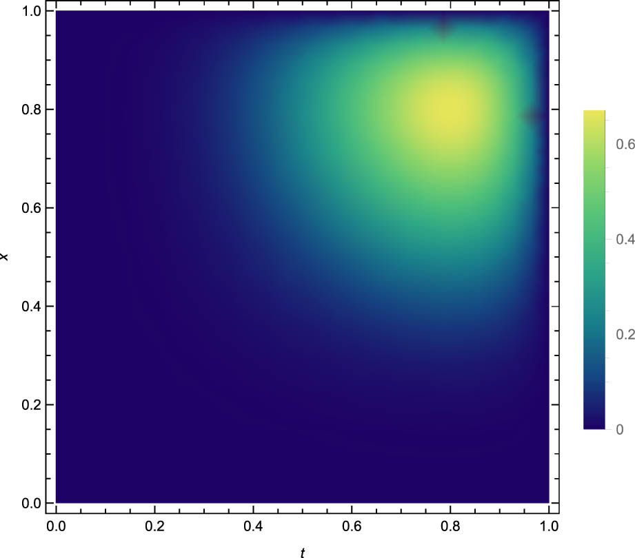
Diagram of the approximate solution for Example 1 using

Diagram of the absolute error for Example 1 using
Example 2
Consider a fractal-fractional advection–diffusion–reaction equation as in Example 1 [14]:
Here, again, we refer the reader to Example 1 [14] for the long expression of
In order to obtain the numerical solution, we need Lemma (2.4) as in ref. [32]. From the numerical result as shown in Table 2, with only few terms of two variables-shifted Legendre polynomials via Ritz approximation, our proposed method is comparable with the method via Berstein polynomials and its operational matrix as in ref. [14], using more terms of polynomials. Similar to Example 1, the calculation is done by using Maple and applying Lemma 2.4 and Corollary 2.5 in ref. [32] and Corollary 2.5 in [43].
Comparison of the maximum absolute errors obtained by proposed method with
| (
|
|
|
MAE [14] |
|
MAE (proposed method) |
|---|---|---|---|---|---|
| (0.75,0.25) | 7 | 7 |
|
2 |
|
| (0.75,0.5) | 7 | 7 |
|
2 |
|
| (0.45,0.35) | 7 | 7 |
|
2 |
|
| (0.65,0.35) | 7 | 7 |
|
2 |
|
5 Conclusion
In this article, we successfully used the Ritz approximation approach to solve fractal-fractional advection–diffusion–reaction equations via two variables-shifted Legendre polynomials. With Ritz approximation, greatly reduces the number of terms of polynomials needed for numerical simulation to obtain the solution for fractal-fractional advection–diffusion–reaction equations. With only few terms of two variables-shifted Legendre polynomials, we were able to obtain the numerical solution with high accuracy. The proposed procedure can be easily extended to solve fractal-fractional advection–diffusion–reaction equations in variable order. Furthermore, we hope to extend the method to tackle the inverse problems related to fractional partial differential equations such as those in ref. [44,45,46], or more complicated scenarios and problems, such as those in ref. [47].
-
Funding information: The authors would like to thank Universiti Teknologi MARA, Johor Branch for supporting this research under Geran Penyelidikan Bestari Vot No. 29000.
-
Author contributions: All authors have accepted responsibility for the entire content of this manuscript and approved its submission.
-
Conflict of interest: The authors state no conflict of interest.
References
[1] Li Z, Yazdani A, Tartakovsky A, Em Karniadakis G. Transport dissipative particle dynamics model for mesoscopic advection–diffusion–reaction problems. J Chem Phys. 2015;143(1): 014101. 10.1063/1.4923254Search in Google Scholar PubMed PubMed Central
[2] Lin J, Reutskiy S, Chen C-S, Lu J. A novel method for solving time-dependent 2D advection–diffusion–reaction equations to model transfer in nonlinear anisotropic media. Commun Comput Phys. 2019;26(1):233–64. 10.4208/cicp.OA-2018-0005Search in Google Scholar
[3] Pudykiewicz JA. Numerical solution of the reaction-advection-diffusion equation on the sphere. J Comput Phys. 2006;213(1):358–90. 10.1016/j.jcp.2005.08.021Search in Google Scholar
[4] Perez LJ, Hidalgo JJ, Dentz M. Reactive random walk particle tracking and its equivalence with the advection–diffusion–reaction equation. Water Resour Res. 2019;55(1):847–55. 10.1029/2018WR023560Search in Google Scholar
[5] Shahid N, Ahmed N, Baleanu D, Saleh Alshomrani A, SajidIqbal M, Aziz-urRehman M, et al. Novel numerical analysis for nonlinear advection-reaction-diffusion systems. Open Phys. 2020;18(1):112–25. 10.1515/phys-2020-0011Search in Google Scholar
[6] AlQurashi MM. Role of fractal-fractional operators in modeling of Rubella epidemic with optimized orders. Open Phys. 2020;18(1):1111–20. 10.1515/phys-2020-0217Search in Google Scholar
[7] Haidong Q, UrRahman M, Arfan M, Laouini G, Ahmadian A, Senu N, et al. Investigating fractal-fractional mathematical model of Tuberculosis (TB) under fractal-fractional Caputo operator. Fractals. 2022;30(5):2240126.10.1142/S0218348X22401260Search in Google Scholar
[8] Abdulwasaa MA, Abdo MS, Shah K, Nofal TA, Panchal SK, Kawale SV, et al. Fractal-fractional mathematical modeling and forecasting of new cases and deaths of COVID-19 epidemic outbreaks in India. Result Phys. 2021;20:103702. 10.1016/j.rinp.2020.103702Search in Google Scholar PubMed PubMed Central
[9] Schumer R, Meerschaert MM, Baeumer B. Fractional advection-dispersion equations for modeling transport at the earth surface. J Geophys Res Earth Surface. 2009;114(F4):F00A07.10.1029/2008JF001246Search in Google Scholar
[10] Hussain M, Haq S. Weighted meshless spectral method for the solutions of multi-term time fractional advection-diffusion problems arising in heat and mass transfer. Int J Heat Mass Transf. 2019;129:1305–16. 10.1016/j.ijheatmasstransfer.2018.10.039Search in Google Scholar
[11] Agarwal R, Jain S, Agarwal RP. Mathematical modeling and analysis of dynamics of cytosolic calcium ion in astrocytes using fractional calculus. J Fractional Calculus Appl. 2018;9(2):1–12. Search in Google Scholar
[12] Atangana A. Fractal-fractional differentiation and integration: Connecting fractal calculus and fractional calculus to predict complex system. Chaos Soliton Fractal. 2017;102:396–406. 10.1016/j.chaos.2017.04.027Search in Google Scholar
[13] Atangana A, Qureshi S. Modeling attractors of chaotic dynamical systems with fractal-fractional operators. Chaos Soliton Fractal. 2019;123:320–37. 10.1016/j.chaos.2019.04.020Search in Google Scholar
[14] Heydari MH, Avazzadeh Z, Yang Y. Numerical treatment of the space-time fractal-fractional model of nonlinear advection–diffusion–reaction equation through the Bernstein polynomials. Fractals. 2020;28:2040001. 10.1142/S0218348X20400010Search in Google Scholar
[15] Abro KA. Role of fractal-fractional derivative on ferromagnetic fluid via fractal Laplace transform: A first problem via fractal-fractional differential operator. Europ J Mechanics-B/Fluids. 2021;85:76–81. 10.1016/j.euromechflu.2020.09.002Search in Google Scholar
[16] Gómez-Aguilar JF, Atangana A. New chaotic attractors: application of fractal-fractional differentiation and integration. Math Meth Appl Sci. 2021;44(4):3036–65. 10.1002/mma.6432Search in Google Scholar
[17] Salomoni VAL, De Marchi N. Numerical solutions of space-fractional advection–diffusion–reaction equations. Fractal Fractional. 2021;6(1):21. 10.3390/fractalfract6010021Search in Google Scholar
[18] Owolabi KM, Atangana A, Akgul A. Modelling and analysis of fractal-fractional partial differential equations: Application to reaction-diffusion model. Alexandr Eng J. 2020;59(4):2477–90. 10.1016/j.aej.2020.03.022Search in Google Scholar
[19] Wang W, Khan MA. Analysis and numerical simulation of fractional model of bank data with fractal-fractional Atangana-Baleanu derivative. J Comput Appl Math. 2020;369:112646. 10.1016/j.cam.2019.112646Search in Google Scholar
[20] Gómez-Aguilar JF. Chaos and multiple attractors in a fractal-fractional Shinriki’s oscillator model. Phys A Stat Mech Appl. 2020;539:122918. 10.1016/j.physa.2019.122918Search in Google Scholar
[21] Gomez-Aguilar JF, Cordova-Fraga T, Abdeljawad T, Khan A, Khan H. Analysis of fractal-fractional Malaria transmission model. Fractals. 2020;28(8):204004110.1142/S0218348X20400411Search in Google Scholar
[22] Meerschaert MM, Tadjeran C. Finite difference approximations for fractional advection-dispersion flow equations. J Comput Appl Math. 2004;172(1):65–77. 10.1016/j.cam.2004.01.033Search in Google Scholar
[23] Chen W, Sun H, Zhang X, Korošak D. Anomalous diffusion modeling by fractal and fractional derivatives. Comput Math Appl. 2010;59(5):1754–8. 10.1016/j.camwa.2009.08.020Search in Google Scholar
[24] Kaharuddin LN, Phang C, Jamaian SS. Solution to the fractional logistic equation by modified Eulerian numbers. European Phys J Plus. 2020;135(2):229. 10.1140/epjp/s13360-020-00135-ySearch in Google Scholar
[25] Loh JR, Phang C, Tay KG. New method for solving fractional partial integro-differential equations by combination of Laplace transform and resolvent kernel method. Chinese J Phys. 2020;67:666–80. 10.1016/j.cjph.2020.08.017Search in Google Scholar
[26] Barikbin Z, Keshavarz E. Solving fractional optimal control problems by new Bernoulli wavelets operational matrices. Optimal Control Appl Meth. 2020;41(4):1188–210. 10.1002/oca.2598Search in Google Scholar
[27] Toh YT, Phang C, Ng YX. Temporal discretization for Caputo-Hadamard fractional derivative with incomplete Gamma function via Whittaker function. Comput Appl Math. 2021;40(8):1–19. 10.1007/s40314-021-01673-6Search in Google Scholar
[28] Phang C, Toh YT, MdNasrudin FS. An operational matrix method based on poly-Bernoulli polynomials for solving fractional delay differential equations. Computation, 2020;8(3):82. 10.3390/computation8030082Search in Google Scholar
[29] Heydari MH, Atangana A, Avazzadeh Z. Chebyshev polynomials for the numerical solution of fractal-fractional model of nonlinear Ginzburg-Landau equation. Eng Comput. 2021;37:1377–88. 10.1007/s00366-019-00889-9Search in Google Scholar
[30] Yadav MP, Agarwal R. Numerical investigation of fractional-fractal Boussinesq equation. Chaos Interdisciplinary J Nonlinear Sci. 2019;29(1):013109. 10.1063/1.5080139Search in Google Scholar PubMed
[31] Solís-Pérez JE, Gómez-Aguilar JF. Variable-order fractal-fractional time delay equations with power, exponential and Mittag-Leffler laws and their numerical solutions. Eng Comput. 2022;38:555–77. 10.1007/s00366-020-01065-0Search in Google Scholar
[32] Heydari MH, Hosseininia M, Avazzadeh Z. An efficient wavelet-based approximation method for the coupled nonlinear fractal-fractional 2d Schrödinger equations. Eng Comput. 2021;37:2129–44. 10.1007/s00366-020-00934-ySearch in Google Scholar
[33] Rashedi K, Adibi H, Dehghan M. Application of the Ritz-Galerkin method for recovering the spacewise-coefficients in the wave equation. Comput Math Appl. 2013;65(12):1990–2008. 10.1016/j.camwa.2013.04.005Search in Google Scholar
[34] Yousefi SA, Lesnic D, Barikbin Z. Satisfier function in Ritz-Galerkin method for the identification of a time-dependent diffusivity. J Inverse Ill-Posed Problems 2012;20(5–6):701–22. 10.1515/jip-2012-0020Search in Google Scholar
[35] Firoozjaee MA, Yousefi SA. A numerical approach for fractional partial differential equations by using Ritz approximation. Appl Math Comput. 2018;338:711–21. 10.1016/j.amc.2018.05.043Search in Google Scholar
[36] Barikbin Z. Two-dimensional Bernoulli wavelets with satisfier function in the Ritz-Galerkin method for the time fractional diffusion-wave equation with damping. Math Sci. 2017;11(3):195–202. 10.1007/s40096-017-0214-4Search in Google Scholar
[37] Barikbin Z, Keshavarz Hedayati E. Exact and approximation product solutions form of heat equation with nonlocal boundary conditions using Ritz-Galerkin method with Bernoulli polynomials basis. Numer Meth Partial Differ Equ. 2017;33(4):1143–58. 10.1002/num.22136Search in Google Scholar
[38] Kanwal A, Phang C, Iqbal U. Numerical solution of fractional diffusion wave equation and fractional Klein-Gordon equation via two-dimensional Genocchi polynomials with a Ritz-Galerkin method. Computation. 2018;6(3):40. 10.3390/computation6030040Search in Google Scholar
[39] Khan MA, Singh MP. A study of two variables Legendre polynomials. Pro Math. 2010;24(47–48):201–23. Search in Google Scholar
[40] Dattoli G, Germano B, Martinelli MR, Ricci PE. A novel theory of Legendre polynomials. Math Comput Modell. 2011;54(1–2):80–87. 10.1016/j.mcm.2011.01.037Search in Google Scholar
[41] Patel VK, Singh S, Singh VK. Two-dimensional shifted Legendre polynomial collocation method for electromagnetic waves in dielectric media via almost operational matrices. Math Meth Appl Sci. 2017;40(10):3698–717. 10.1002/mma.4257Search in Google Scholar
[42] Hesameddini E, Shahbazi M. Two-dimensional shifted Legendre polynomials operational matrix method for solving the two-dimensional integral equations of fractional order. Appl Math Comput. 2018;322:40–54. 10.1016/j.amc.2017.11.024Search in Google Scholar
[43] Hosseininia M, Heydari MH. Legendre wavelets for the numerical solution of nonlinear variable-order time fractional 2d reaction-diffusion equation involving Mittag-Leffler non-singular kernel. Chaos Soliton Fractal. 2019;127:400–7. 10.1016/j.chaos.2019.07.017Search in Google Scholar
[44] Taghavi A, Babaei A, Mohammadpour A. A stable numerical scheme for a time fractional inverse parabolic equation. Inverse Problems Sci Eng. 2017;25(10):1474–91. 10.1080/17415977.2016.1267169Search in Google Scholar
[45] Babaei A, Banihashemi S. A stable numerical approach to solve a time-fractional inverse heat conduction problem. Iranian J Sci Technol Trans A Sci. 2018;42(4):2225–36. 10.1007/s40995-017-0360-4Search in Google Scholar
[46] Babaei A, Banihashemi S. Reconstructing unknown nonlinear boundary conditions in a time-fractional inverse reaction-diffusion-convection problem. Numer Meth Partial Differ Equ. 2019;35(3):976–92. 10.1002/num.22334Search in Google Scholar
[47] Salomoni VA, De Marchi N. A fractional approach to fluid flow and solute transport within deformable saturated porous media. Int J Comput Materials Sci Eng. 2022;11(3):2250003. 10.1142/S2047684122500038Search in Google Scholar
© 2023 the author(s), published by De Gruyter
This work is licensed under the Creative Commons Attribution 4.0 International License.
Articles in the same Issue
- Regular Articles
- Dynamic properties of the attachment oscillator arising in the nanophysics
- Parametric simulation of stagnation point flow of motile microorganism hybrid nanofluid across a circular cylinder with sinusoidal radius
- Fractal-fractional advection–diffusion–reaction equations by Ritz approximation approach
- Behaviour and onset of low-dimensional chaos with a periodically varying loss in single-mode homogeneously broadened laser
- Ammonia gas-sensing behavior of uniform nanostructured PPy film prepared by simple-straightforward in situ chemical vapor oxidation
- Analysis of the working mechanism and detection sensitivity of a flash detector
- Flat and bent branes with inner structure in two-field mimetic gravity
- Heat transfer analysis of the MHD stagnation-point flow of third-grade fluid over a porous sheet with thermal radiation effect: An algorithmic approach
- Weighted survival functional entropy and its properties
- Bioconvection effect in the Carreau nanofluid with Cattaneo–Christov heat flux using stagnation point flow in the entropy generation: Micromachines level study
- Study on the impulse mechanism of optical films formed by laser plasma shock waves
- Analysis of sweeping jet and film composite cooling using the decoupled model
- Research on the influence of trapezoidal magnetization of bonded magnetic ring on cogging torque
- Tripartite entanglement and entanglement transfer in a hybrid cavity magnomechanical system
- Compounded Bell-G class of statistical models with applications to COVID-19 and actuarial data
- Degradation of Vibrio cholerae from drinking water by the underwater capillary discharge
- Multiple Lie symmetry solutions for effects of viscous on magnetohydrodynamic flow and heat transfer in non-Newtonian thin film
- Thermal characterization of heat source (sink) on hybridized (Cu–Ag/EG) nanofluid flow via solid stretchable sheet
- Optimizing condition monitoring of ball bearings: An integrated approach using decision tree and extreme learning machine for effective decision-making
- Study on the inter-porosity transfer rate and producing degree of matrix in fractured-porous gas reservoirs
- Interstellar radiation as a Maxwell field: Improved numerical scheme and application to the spectral energy density
- Numerical study of hybridized Williamson nanofluid flow with TC4 and Nichrome over an extending surface
- Controlling the physical field using the shape function technique
- Significance of heat and mass transport in peristaltic flow of Jeffrey material subject to chemical reaction and radiation phenomenon through a tapered channel
- Complex dynamics of a sub-quadratic Lorenz-like system
- Stability control in a helicoidal spin–orbit-coupled open Bose–Bose mixture
- Research on WPD and DBSCAN-L-ISOMAP for circuit fault feature extraction
- Simulation for formation process of atomic orbitals by the finite difference time domain method based on the eight-element Dirac equation
- A modified power-law model: Properties, estimation, and applications
- Bayesian and non-Bayesian estimation of dynamic cumulative residual Tsallis entropy for moment exponential distribution under progressive censored type II
- Computational analysis and biomechanical study of Oldroyd-B fluid with homogeneous and heterogeneous reactions through a vertical non-uniform channel
- Predictability of machine learning framework in cross-section data
- Chaotic characteristics and mixing performance of pseudoplastic fluids in a stirred tank
- Isomorphic shut form valuation for quantum field theory and biological population models
- Vibration sensitivity minimization of an ultra-stable optical reference cavity based on orthogonal experimental design
- Effect of dysprosium on the radiation-shielding features of SiO2–PbO–B2O3 glasses
- Asymptotic formulations of anti-plane problems in pre-stressed compressible elastic laminates
- A study on soliton, lump solutions to a generalized (3+1)-dimensional Hirota--Satsuma--Ito equation
- Tangential electrostatic field at metal surfaces
- Bioconvective gyrotactic microorganisms in third-grade nanofluid flow over a Riga surface with stratification: An approach to entropy minimization
- Infrared spectroscopy for ageing assessment of insulating oils via dielectric loss factor and interfacial tension
- Influence of cationic surfactants on the growth of gypsum crystals
- Study on instability mechanism of KCl/PHPA drilling waste fluid
- Analytical solutions of the extended Kadomtsev–Petviashvili equation in nonlinear media
- A novel compact highly sensitive non-invasive microwave antenna sensor for blood glucose monitoring
- Inspection of Couette and pressure-driven Poiseuille entropy-optimized dissipated flow in a suction/injection horizontal channel: Analytical solutions
- Conserved vectors and solutions of the two-dimensional potential KP equation
- The reciprocal linear effect, a new optical effect of the Sagnac type
- Optimal interatomic potentials using modified method of least squares: Optimal form of interatomic potentials
- The soliton solutions for stochastic Calogero–Bogoyavlenskii Schiff equation in plasma physics/fluid mechanics
- Research on absolute ranging technology of resampling phase comparison method based on FMCW
- Analysis of Cu and Zn contents in aluminum alloys by femtosecond laser-ablation spark-induced breakdown spectroscopy
- Nonsequential double ionization channels control of CO2 molecules with counter-rotating two-color circularly polarized laser field by laser wavelength
- Fractional-order modeling: Analysis of foam drainage and Fisher's equations
- Thermo-solutal Marangoni convective Darcy-Forchheimer bio-hybrid nanofluid flow over a permeable disk with activation energy: Analysis of interfacial nanolayer thickness
- Investigation on topology-optimized compressor piston by metal additive manufacturing technique: Analytical and numeric computational modeling using finite element analysis in ANSYS
- Breast cancer segmentation using a hybrid AttendSeg architecture combined with a gravitational clustering optimization algorithm using mathematical modelling
- On the localized and periodic solutions to the time-fractional Klein-Gordan equations: Optimal additive function method and new iterative method
- 3D thin-film nanofluid flow with heat transfer on an inclined disc by using HWCM
- Numerical study of static pressure on the sonochemistry characteristics of the gas bubble under acoustic excitation
- Optimal auxiliary function method for analyzing nonlinear system of coupled Schrödinger–KdV equation with Caputo operator
- Analysis of magnetized micropolar fluid subjected to generalized heat-mass transfer theories
- Does the Mott problem extend to Geiger counters?
- Stability analysis, phase plane analysis, and isolated soliton solution to the LGH equation in mathematical physics
- Effects of Joule heating and reaction mechanisms on couple stress fluid flow with peristalsis in the presence of a porous material through an inclined channel
- Bayesian and E-Bayesian estimation based on constant-stress partially accelerated life testing for inverted Topp–Leone distribution
- Dynamical and physical characteristics of soliton solutions to the (2+1)-dimensional Konopelchenko–Dubrovsky system
- Study of fractional variable order COVID-19 environmental transformation model
- Sisko nanofluid flow through exponential stretching sheet with swimming of motile gyrotactic microorganisms: An application to nanoengineering
- Influence of the regularization scheme in the QCD phase diagram in the PNJL model
- Fixed-point theory and numerical analysis of an epidemic model with fractional calculus: Exploring dynamical behavior
- Computational analysis of reconstructing current and sag of three-phase overhead line based on the TMR sensor array
- Investigation of tripled sine-Gordon equation: Localized modes in multi-stacked long Josephson junctions
- High-sensitivity on-chip temperature sensor based on cascaded microring resonators
- Pathological study on uncertain numbers and proposed solutions for discrete fuzzy fractional order calculus
- Bifurcation, chaotic behavior, and traveling wave solution of stochastic coupled Konno–Oono equation with multiplicative noise in the Stratonovich sense
- Thermal radiation and heat generation on three-dimensional Casson fluid motion via porous stretching surface with variable thermal conductivity
- Numerical simulation and analysis of Airy's-type equation
- A homotopy perturbation method with Elzaki transformation for solving the fractional Biswas–Milovic model
- Heat transfer performance of magnetohydrodynamic multiphase nanofluid flow of Cu–Al2O3/H2O over a stretching cylinder
- ΛCDM and the principle of equivalence
- Axisymmetric stagnation-point flow of non-Newtonian nanomaterial and heat transport over a lubricated surface: Hybrid homotopy analysis method simulations
- HAM simulation for bioconvective magnetohydrodynamic flow of Walters-B fluid containing nanoparticles and microorganisms past a stretching sheet with velocity slip and convective conditions
- Coupled heat and mass transfer mathematical study for lubricated non-Newtonian nanomaterial conveying oblique stagnation point flow: A comparison of viscous and viscoelastic nanofluid model
- Power Topp–Leone exponential negative family of distributions with numerical illustrations to engineering and biological data
- Extracting solitary solutions of the nonlinear Kaup–Kupershmidt (KK) equation by analytical method
- A case study on the environmental and economic impact of photovoltaic systems in wastewater treatment plants
- Application of IoT network for marine wildlife surveillance
- Non-similar modeling and numerical simulations of microploar hybrid nanofluid adjacent to isothermal sphere
- Joint optimization of two-dimensional warranty period and maintenance strategy considering availability and cost constraints
- Numerical investigation of the flow characteristics involving dissipation and slip effects in a convectively nanofluid within a porous medium
- Spectral uncertainty analysis of grassland and its camouflage materials based on land-based hyperspectral images
- Application of low-altitude wind shear recognition algorithm and laser wind radar in aviation meteorological services
- Investigation of different structures of screw extruders on the flow in direct ink writing SiC slurry based on LBM
- Harmonic current suppression method of virtual DC motor based on fuzzy sliding mode
- Micropolar flow and heat transfer within a permeable channel using the successive linearization method
- Different lump k-soliton solutions to (2+1)-dimensional KdV system using Hirota binary Bell polynomials
- Investigation of nanomaterials in flow of non-Newtonian liquid toward a stretchable surface
- Weak beat frequency extraction method for photon Doppler signal with low signal-to-noise ratio
- Electrokinetic energy conversion of nanofluids in porous microtubes with Green’s function
- Examining the role of activation energy and convective boundary conditions in nanofluid behavior of Couette-Poiseuille flow
- Review Article
- Effects of stretching on phase transformation of PVDF and its copolymers: A review
- Special Issue on Transport phenomena and thermal analysis in micro/nano-scale structure surfaces - Part IV
- Prediction and monitoring model for farmland environmental system using soil sensor and neural network algorithm
- Special Issue on Advanced Topics on the Modelling and Assessment of Complicated Physical Phenomena - Part III
- Some standard and nonstandard finite difference schemes for a reaction–diffusion–chemotaxis model
- Special Issue on Advanced Energy Materials - Part II
- Rapid productivity prediction method for frac hits affected wells based on gas reservoir numerical simulation and probability method
- Special Issue on Novel Numerical and Analytical Techniques for Fractional Nonlinear Schrodinger Type - Part III
- Adomian decomposition method for solution of fourteenth order boundary value problems
- New soliton solutions of modified (3+1)-D Wazwaz–Benjamin–Bona–Mahony and (2+1)-D cubic Klein–Gordon equations using first integral method
- On traveling wave solutions to Manakov model with variable coefficients
- Rational approximation for solving Fredholm integro-differential equations by new algorithm
- Special Issue on Predicting pattern alterations in nature - Part I
- Modeling the monkeypox infection using the Mittag–Leffler kernel
- Spectral analysis of variable-order multi-terms fractional differential equations
- Special Issue on Nanomaterial utilization and structural optimization - Part I
- Heat treatment and tensile test of 3D-printed parts manufactured at different build orientations