Optimizing condition monitoring of ball bearings: An integrated approach using decision tree and extreme learning machine for effective decision-making

Riadh Euldji; Mouloud Bouamhdi; Redha Rebhi; Mourad Bachene; Omolayo M. Ikumapayi; Ayad Q. Al-Dujaili; Ahmed I. Abdulkareem; Amjad J. Humaidi; Younes Menni

doi:10.1515/phys-2022-0239

Article Open Access

Optimizing condition monitoring of ball bearings: An integrated approach using decision tree and extreme learning machine for effective decision-making

Riadh Euldji , Mouloud Bouamhdi , Redha Rebhi , Mourad Bachene , Omolayo M. Ikumapayi , Ayad Q. Al-Dujaili , Ahmed I. Abdulkareem , Amjad J. Humaidi and Younes Menni

Published/Copyright: June 12, 2023

Published by

Become an author with De Gruyter Brill

Submit Manuscript Author Information Explore this Subject

From the journal Open Physics Volume 21 Issue 1

Abstract

This article presents a study on condition monitoring and predictive maintenance, highlighting the importance of tracking ball bearing condition to estimate their Remaining Useful Life (RUL). The study proposes a methodology that combines three algorithms, namely Variational Mode Decomposition (VMD), Decision Tree (DT), and Extreme Learning Machine (ELM), to extract pertinent features and estimate RUL using vibration signals. To improve the accuracy of the method, the VMD algorithm is used to reduce noise from the original vibration signals. The DT algorithm is then employed to extract relevant features, which are fed into the ELM algorithm to estimate the RUL of the ball bearings. The effectiveness of the proposed approach is evaluated using ball bearing data sets from the PRONOSTIA platform. Overall, the results demonstrate that the suggested methodology successfully tracks the ball bearing condition and estimates RUL using vibration signals. This study provides valuable insights into the development of predictive maintenance systems that can assist decision-makers in planning maintenance activities. Further research could explore the potential of this methodology in other industrial applications and under different operating conditions.

Keywords: condition monitoring; ball bearings; variational mode decomposition; decision tree; extreme learning machines

1 Introduction

Rotating machines consist of vital components known as bearings, and their degradation can significantly impact dependability, availability, security, maintenance, ecology, and economy. Such effects directly influence the productivity and quality of the machine’s performance. Given the critical nature of bearings, reliable information about their state is essential. Vibration condition monitoring is a widely used method to evaluate the condition of bearings, and detecting flaws and predicting the Remaining Usable Life (RUL) of bearings are of particular interest to manufacturers and researchers. The process of vibration condition monitoring involves three primary stages, namely data acquisition, data processing, and maintenance decision-making, each of which is critical for ensuring the effectiveness of the approach. As such, efforts are continually being made to improve each stage of the process to enhance the overall reliability and accuracy of vibration condition monitoring for bearings [1,2,3].

Machine learning techniques can be used to extract useful information that aids decision-making from the vast amount of measured and stored data. Large volumes of data can be mined for knowledge using machine learning. In complicated systems where degradation processes are challenging to connect using a physics or statistical model, machine learning can handle prediction issues. In the literature, numerous strategies and methods for anomalies prediction have been put forth and assessed. SVM (Support Vector Machines) [4,5,6,7], Extreme Learning Machines (ELM) [8,9,10], and neural networks [11,12,13,14,15,16] are among them. A hybrid strategy uses different algorithms to enhance the performance of RUL prediction. For more details, Table 1 highlights the most significant studies that examined the state of machine learning applications in various algorithms at the time and showed potential future applications.

Table 1

Review the current status and future opportunities for machine learning applications with various algorithms

Authors	Highlights
Peng et al. [17]	To offer insights into the development of Decision Tree (DT) technology for rolling bearings, a comprehensive literature review was conducted, focusing on the fundamental aspects of DT construction, including detection, modeling, and Prognostics Health Management. The review provided a historical perspective of DT technology and identified the key challenges associated with establishing a robust DT technique for rolling bearings. Various proposals for future research directions were also evaluated to address the identified challenges and improve the performance of DT-based condition monitoring for rolling bearings. Overall, this study provides a valuable overview of the evolution and potential of DT technology in the context of rolling bearing condition monitoring, paving the way for further developments in the field
Xu and Saleh [18]	Several associated models and algorithms are noted along with an overview of various machine learning classes, subclasses, or tasks. Review machine learning’s use in applications for dependability and safety next. Each category and subcategory’s publications were examined in depth, and a brief overview of deep learning’s (DL) application is included to illustrate the technology’s rising popularity and unique benefits. Finally, a number of intriguing opportunities to apply machine learning to improved reliability and safety issues have been found
Bertolini et al. [19]	They examined the potential benefits and potential drawbacks of machine learning algorithms used in process management
Soni and Kumar [20]	This comprehensive review study provides a well-structured summary of the extensive research on the integration of machine learning methods within the rapidly evolving cloud computing paradigm. The study offers a comprehensive assessment of the literature, focusing on the latest cloud computing paradigms, including cloud, edge, fog, mist, Internet of Things, SDN (Software-Defined Networking), cybertwin, and industrial 4.0 (IIoT). In addition, the study explores how these paradigms can be effectively combined with machine learning techniques to enhance their performance and capabilities. By consolidating a large volume of research, this study offers valuable insights into the latest developments and potential applications of machine learning within the cloud computing paradigm, making it a valuable resource for researchers and practitioners in the field
Avci et al. [21]	Vibration-based Structural Damage Detection (SDD) techniques have traditionally relied on conventional approaches, with limited consideration of the potential benefits of machine learning and DL methods. This study aims to bridge this gap by providing an in-depth analysis of the latest machine learning and DL algorithms for vibration-based SDD, alongside a review of the key aspects of conventional approaches. Specifically, the study offers a comprehensive examination of the potential applications of machine learning and DL algorithms for structural damage diagnosis in civil constructions, highlighting their unique advantages and limitations. By exploring the latest developments and trends in this field, this study sheds new light on the potential of machine learning and DL for vibration-based SDD, paving the way for further research and innovation in this critical area
Li et al. [22]	In this paper, the authors present a systematic review of research advancements in monitoring tool breakage during machining processes, which is a critical aspect of preventing unexpected tool failure and potential production mishaps. The study offers a detailed overview of the methodology used for signal acquisition, feature extraction, and decision-making in tool breakage monitoring, which is compared to relevant methods for instrument wear monitoring. By exploring the latest developments in this field, this study provides a valuable resource for researchers and practitioners seeking to enhance tool breakage monitoring in machining processes. The authors’ methodical approach and critical analysis of the current state of the art in this area makes this study a valuable contribution to the field, providing new insights and identifying areas for further research and development
Ntemi et al. [23]	The authors of these studies have conducted a comprehensive evaluation of the latest advances in infrastructure monitoring and rapid quality diagnostics for computer numerical controlled (CNC) machining operations. With great attention to detail, they have analyzed the most current developments in these areas, offering a valuable resource for researchers and practitioners seeking to enhance CNC machining operations. By exploring the latest technologies and techniques, this research provides insights into how to improve the accuracy, reliability, and efficiency of CNC machining operations, and lays the groundwork for future innovations in this field. The authors’ careful and thorough analysis of the state of the art in infrastructure monitoring and quick quality diagnostics makes this study an essential reference for anyone working in CNC machining
van Dinter et al. [24]	42 primary papers were examined as part of a systematic evaluation of the literature on predictive maintenance employing digital twins using active learning technology
Zhao et al. [25]	The use of modern DL models for machine health monitoring tasks has been carefully reviewed.
Gangsar and Tiwari [26]	In this study, the authors conducted a comprehensive investigation into several problems associated with induction motors. They employed traditional time and spectrum signal analysis techniques to examine the two most valuable types of signals for motor diagnosis, namely vibration and current. Additionally, the study provides an overview of the latest research and advancements in signal-based automation for condition monitoring, which can aid in detecting and diagnosing electrical and mechanical defects in induction motors. By exploring the most recent developments in this field, the authors offer valuable insights into how to enhance the accuracy and efficiency of condition monitoring and fault diagnosis for induction motors. This research represents a significant contribution to the field, offering a detailed analysis of signal analysis and condition monitoring of induction motors and providing a roadmap for future research and development.
Hakim et al. [27]	The aim of this review study was to offer a thorough and all-encompassing summary of the use of DL in bearing error diagnosis. To achieve this, the authors examined various DL techniques that are commonly used for bearing fault detection, including convolutional neural networks, recurrent neural networks, autoencoders, and generative adversarial networks. By exploring the most frequently employed DL methods, the authors provide valuable insights into how to effectively diagnose bearing faults and improve the overall reliability and performance of rotating machinery. This review study provides a solid foundation for future research in this area, offering a comprehensive analysis of DL-based bearing diagnosis that can guide the development of more effective techniques and tools for fault detection and diagnosis
Huang et al. [28]	The references analyzed were divided into two groups: enhanced SVM techniques and their use in RUL estimation
Liu et al. [29]	The authors aimed to summarize the methods for predicting the RUL of affordances, which can be broadly classified into three categories: physical model-based methods, statistical methods, and data-driven methods based on condition monitoring. By comparing the advantages and disadvantages of each of these methods, the authors also provide some guidance for selecting an appropriate prediction method for practical applications
Si et al. [30]	The authors reviewed current RUL estimation modeling advancements. The review’s main focus is on statistical data-driven methodologies that only use readily accessible historical observed data and statistical models. The methods are divided into two main categories of models: those that rely on knowledge about the asset’s state that has been directly seen and those that do not

Numerous earlier studies focused on predicting RUL using just one feature. On the other hand, the DT is an effective tool for extracting important features. For this reason, it is suggested to use all the features extracted from the DT to estimate the RUL. The goal of this study is to develop a novel data-driven methodology for monitoring and predicting ball-bearing RUL. In order to cut down on noise, the vibration signals are first denoised using the Variational Mode Decomposition (VMD). Second, employ the DT algorithm to extract useful knowledge from two independent data sets made up of original signals and denoised signals. The RUL is modeled by regression using the ELM, which is the third step. Finally, performance criteria is used to assess the effectiveness of the given methodology. This article’s main contributions are as follows: (i) the suggested methodology offers a tool for monitoring the condition of ball bearings, (ii) the relevant features can be extracted using the DT technique, and (iii) combining the DT and ELM techniques enables estimation of the RUL based on various DT criteria. The rest of this essay is structured as follows: Three techniques (VMD, DT, and ELM) are briefly reviewed in the second section. The results, including comparisons, are covered in the third section. The most significant points made are highlighted in the final section.

2 Methodology

The suggested methodology’s flowchart to monitor the ball bearings’ health and predict the RUL is shown in Figure 1.

Figure 1

Flowchart of the proposed methodology.

During operation, bearings produce vibrations that can be monitored using indicators like RMS and peak value. By plotting these indicators over time, it is possible to observe the trend of the bearing’s degradation (Figure 2). Accurately estimating the current and future health of a bearing is crucial to extend its operation. By predicting the RUL of the bearing, which refers to the time until the machine ceases operating, appropriate maintenance decisions can be made.

Figure 2

Degradation indicator over time.

Before using the proposed methodology, some concepts must be clarified. Figure 2 depicts the evolution of a degradation indicator over RT (Run-Time). The alert point is denoted by AP , which is the intersection of the deterioration index curve and the alert threshold line; the current point is denoted by P . The danger point, indicated by DP , is the intersection of the deterioration indicator curve and the danger threshold line. Finally, t stands for the current time, t f for the failure time, and RUL for the RUL.

2.1 VMD algorithm

In ball bearings, for example, vibrations and noise, in the form of periodic impulses created when the balls pass over a flaw in the rings, are examples of complex and non-tationary vibration signals, and impulsive signatures are typically concealed by stochastic noise. Signal processing techniques are employed to improve follow-up on the degradation in order to lessen the impact of this noise. One of the newest methods for signal decomposition used to lower noise is VMD, which is similar to Empirical Modes Decomposition (EMD). As a brand-new technique for self-adapting signal decomposition, Dragomiretskiy and Zosso introduced VMD in 2014. The original signal can be divided using the VMD approach into a limited number of signals known as IMFs (Intrinsic Mode Functions) [31], which are defined as follows:

(1) x n = ∑ i = 1 k u k ( t ) + res ( t ) .

Here, x n represents the original signal, { u k } = { u 1 , u 2 , … , u n } represent the decomposition signals, and res is the residual signal following optimization. The decomposition procedure involves resolving the following optimization problem:

(2) min { u k } , { ω k } ∑ k ∂ t δ ( t ) + j π t u k ( t ) e − j ω k t 2 2 , subject to ∑ k u k = x n .

Here, { u k } represents the IMFs set, { ω k } represents the center frequencies of each { u k } , δ ( t ) represents an impulse function, and k is a modal component. By including both a quadratic penalty term ( α ) and Lagrangian multipliers ( λ ), the augmented Lagrangian function ( λ ) is addressed in order to minimize Eq. (2):

(3) L ( { u k } , { ω k } , λ ) ≔ α ∑ k ∂ t δ ( t ) + j π t u k ( t ) e − j ω k t 2 2 + x n ( t ) − ∑ k u k ( t ) 2 2 + ⟨ λ ( t ) , x n ( t ) − ∑ k u k ( t ) ⟩ .

The solution is achieved by optimizing each IMF’s center frequency and bandwidth. The frequency u ˆ k updating procedures can be stated as follows:

(4) u ̑ k n + 1 ( ω ) ← x ̑ n ( ω ) ∑ i ⟨ k u ̑ k n + 1 ( ω ) − ∑ i ⟩ k u ̑ k n ( ω ) + λ ̑ ( ω ) / 2 1 + 2 α ( ω − ω k n ) 2 .

Here, u ˆ k n + 1 ( ω ) , x n ( ω ) , and λ ˆ ( ω ) denote the Fourier transformations, respectively, for u ˆ k n , x n ( t ) , and λ ( t ) . These are ω k n + 1 's updating equations:

(5) ω k n + 1 = ∫ 0 ∞ ω | u ̑ k ( ω ) | 2 d ω ∫ 0 ∞ | u ̑ k ( ω ) | 2 d ω .

The VMD process is terminated as soon as the relative error ε drops below the convergence tolerance:

(6) e = ∑ k ‖ u ̑ k n + 1 − u ̑ k n ‖ 2 2 ‖ u ̑ k n ‖ 2 2 ⟨ ε .

2.2 DT algorithm

To categorize data, DT are frequently utilized. The goal of classification is to categorize samples using a model created from a different data source. The latter consists of a collection of decision-making classes and predictive features. It is necessary to define the classes and characteristics that make up the data collection before building the DT. Leaf, node, and branch components make up a DT. An attribute, also known as a classified object property, is represented by each tree node. Each leaf of the tree represents a class, and each branch represents a potential node attribute value [32].

The foundation of this tree’s creation is the extraction of information from data using classification techniques. We cite the following algorithms for the construction tree: CART [33], ID3 [34], and C4.5 [35].

In this study, DTs are built using the C4.5 algorithm. WEKA uses this algorithm to create the J48 classifier. An overview of the C4.5 DT is provided in this section. The supervised learning algorithm C4.5 chooses attributes based on the following criteria [32]:

If X = { X 1 , X 2 , … , X n } is a set of attributes, C = { C 1 , C 2 , … , C k } is a set of classes, the number of attributes is given by n , while the number of classes | C j | is given by k . j = 1,2 , … , k represents the sample number that falls within the class C j . The collection of training examples is denoted by T , while the number of examples in total is | T | .

Entropy, which is defined as the amount of data required to determine the class of a T element, is as follows [32]:

(7) Info ( T ) = − ∑ i = 1 k | C j | | T | log 2 | C j | | T | .

Entropy is minimum when the node is pure. All samples are in the same class, and maximum when the examples are evenly distributed. The quantity of data needed to determine a T element’s class after obtaining its attribute value X i is known as conditional entropy and is defined as:

(8) Info ( X i , T ) = − ∑ i = 1 n | T i | | T | · ∑ j = 1 k | C j | | T i | log 2 | C j | | T i | .

Information gain is a metric used to measure the quality of a split. The most significant attribute can be chosen using this criterion. In comparison to the other traits, the chosen attribute has the most advantage. It is given as follows:

(9) Gain ( X i , T ) = Info ( T ) − Info ( X i , T ) .

The gain ratio is a standard for correcting the gain of entropy’s slant while accounting for the quantity of attribute values and the proportion of these values in the data. The details are as follows:

(10) GR ( X i , T ) = Gain ( X i T ) Split info ( X i , T ) ,

with:

(11) Split info ( X i , T ) = − ∑ i = 1 n | T i | | T | log 2 | T i | | T | .

The selected predictive attribute maximizes the gain ratio.

2.3 ELM algorithm

ELMs are frequently utilized in machine learning due to their fast-learning capabilities and simplicity. ELM is a single hidden layer feedforward neural network that is trained differently than conventional network training methods [36,37,38]. In this section, ELM is briefly described.

Given N different training samples ( x i , t i ) ; i = 1,2 , . . . , N , an ELM’s output is expressed as:

(12) y i = ∑ i = 1 N ∼ β i f i ( x j ) = ∑ i = 1 N ∼ β i f i ( a i · x j + b i ) ,

where j = 1,2 , . . . , N , N ∼ and f i stand for the number of hidden neurons and the function of neuron activation, respectively. The ith hidden neuron is connected to a vector called a i that contains input layer weights.

The jth input sample’s vector is represented by x j , a bias is represented by b i , the ith hidden neuron’s output layer weight is represented by β i , and the training sample number is represented by N . Eq. (12) can be written as follows:

(13) H β = Y ,

Where

(14) H = f 1 ( a 1 x 1 + b 1 ) . . . f N ∼ ( a N ∼ x 1 + b N ∼ ) . . . . . . . . . . f 1 ( a 1 x N + b 1 ) . . . f N ∼ ( a N ∼ x N + b N ∼ ) N × N ∼ ; β = β 1 T . . β N ∼ T N ∼ × m ; Y = y 1 T . . y N T N × m .

where H represents the hidden layer’s output matrix, and β stands for the output weights that can be calculated analytically by obtaining the following least square solution:

(15) β ̑ = H † Y .

2.4 Data collection and features extraction

The PRONOSTIA platform [39] was utilized to gather the data for this investigation, as shown in Figure 3. This platform’s goal is to deliver accurate experimental data that can be utilized to track and describe how ball bearings degrade over the course of their full operational life. Several run-to-failure experiments were conducted by applying radial loads on ball bearings that exceeded the permitted loads to accelerate their degradation.

Figure 3

PRONOSTIA Platform.

In this study, we focus on the vibration signals that were measured during the operating conditions at 1,800 rpm rotation and 4,000 N radial load generated by a hydraulic jack. NSK 6804DD bearings were tested, which possess the ability to function at a maximum velocity of 13,000 rpm.

To collect monitoring data, high-frequency accelerometers, specifically DYTRAN3035B, were attached to the housing of the bearing being tested. One accelerometer is horizontally placed, while the other is vertically placed, allowing them to measure both horizontal and vertical accelerations. These accelerometers are connected to a data acquisition card, the NI DAQCard-9174, which provides monitoring data to the user. The acceleration measurement unit is g, where 1 g = 9.81 m/s². Vibration signals were acquired using two accelerometers and the following parameters: Sampling frequency is 25.6 kHz , Recordings: 2,560 samples (i.e., 1 / 10 s ) are recorded every 10 seconds.

During operation, rotating machines produce vibrations. The high level of these vibrations is due to the deterioration of the condition of its components. For this, statistical indicators, called features, are used to track the health status of these components.

From each vibration signal, 15 statistical features are taken out in order to monitor the condition of the ball bearings. These features can be divided into two subsets. The first subset has proven its effectiveness, such as RMS (Root Mean Square), Peak, Kurtosis, CF (Crest factor), and KF (K factor) [32], while the second subset can be used as a supplement to the first subsets: Rang, mean, STD (Standard Deviation), VAR (Variance), ADEV (Average Deviation), Skewness, Margin, RA (Root Amplitude), IF (Impulse factor), and shape. Table 2 gives the mathematical description of these features [40,41], and Figure 4 depicts their progression over time.

Table 2

Features described mathematically

Features	Description
Range	Range = max ( x i ) − min ( x i )
Mean	Mean = ∑ i = 1 N x i N
Peak	Peak = max \| x i \|
Root amplitude (RA)	RA = ∑ i = 1 N \| x i \| N 2
Root mean square (RMS)	RMS = ∑ i = 1 N x i 2 N
Average deviation (ADEV)	ADEV = ∑ i = 1 N \| x i − Mean \| N
Variation (VAR)	VAR = ∑ i = 1 N ( x i − Mean ) 2 N
Standard deviation (STD)	STD = ∑ i = 1 N ( x i − Mean ) 2 N − 1
Skewness	Skewness = ∑ i = 1 N ( x i − Mean ) 3 ( N − 1 ) · ST D 3
Kurtosis	Kurtosis = ∑ i = 1 N ( x i − Mean ) 4 ( N − 1 ) · ST D 4
Crest factor (CF)	CF = Peak RMS
K Factor (KF)	KF = Peak · RMS
Margin	Margin = Peak RA
Shape	Shape = RMS Margin
Impulse factor (IF)	IF = Peak Margin

Figure 4

Features over time.

3 Results and discussion

In the fault detection process, an anomaly can be detected if a feature exceeds a predetermined threshold. Standards (like ISO10816) or personal experience can be used to set thresholds. However, experience has shown that setting two thresholds for warning and alert is the best approach.

In this work, the warning and alert thresholds are determined as follows: the warning threshold is 2× rms0, and the alert threshold is 10× rms0 where rms0 is the average of the RMS values of the vibration signals measured at the start of the operation.

Under this approach, thresholds are placed in the RMS evolution curve (Figure 5) to categorize the remaining RMS values into the following states: normal, abnormal, and danger. This figure depicts three key points: A, B, and C. Point A signifies the normal operational condition when no defects are detected. Point B, on the other hand, denotes the alarm point, which is where the warning threshold line intersects with the degradation indicator curve. Lastly, Point C is the danger point, where the alert threshold line intersects with the degradation indicator curve.

Figure 5

RMS over time for original signal.

3.1 Denoised signals by the VMD approach

To identify features relevant that help in decision-making when the condition monitoring of ball bearings, two independent data sets are formed from original signals and denoised signals, and then, the features are extracted from these signals. The denoised signals are obtained by applying the VMD approach to the original signals as described earlier. VMD approach decomposes the original signal into a finite number of signals so-called IMFs. The sum of IMFs is the denoised signal. To validate the similarities between denoised signal and original signal, bias has been used. The bias is the difference average [42] and is defined as follows:

(16) Bias = 1 N ∑ i = 1 N ( y IMFs − y Oi ) ,

where y IMFs represents the denoised signal, and y Oi represents the original signal. To determine the number of criteria, we perform the following steps:

First, the maximum number of IMFs for a signal is set at 20 for VMD decomposition. Then, the Bias criterion is used to verify the similarities between the sum of IMFs and the original signal. Then, the curve of bias over the mode number is plotted. Finally, the steady-state values of the bias criterion are selected as the number of IMFs. In this work, the estimated number of IMFs is 5 .

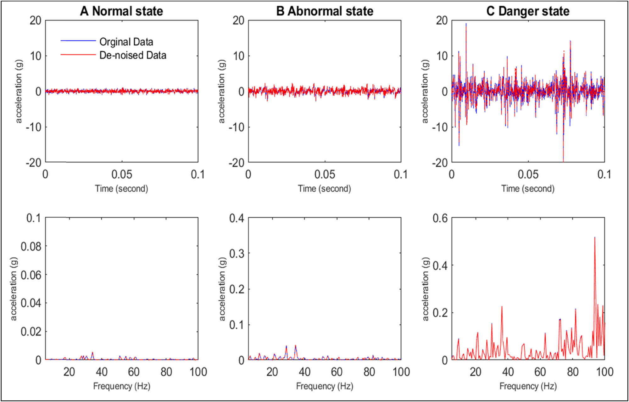
Figure 6 shows three frequency spectrums and the corresponding vibration signals (original and denoised) recorded by a radial accelerometer for three points (Figure 5): A normal, B abnormal, and C danger. Peaks in the spectrum indicate an increase in vibration above normal, as well as a deterioration in the condition of the ball bearings.

Figure 6

Time signals and their spectrums for three states (normal, abnormal, and danger), 1 g = 9.81 m/s².

The features of the original and denoised signals for three different states (normal, abnormal, and danger) over time are depicted in Figure 7. The figure illustrates that the feature values of the two signals are quite similar to one another.

Figure 7

Features over time for three states (A, Normal; B, Abnormal; C, Danger).

Figure 8 shows that the RMS feature values of both signals, namely the actual and the one processed with VMD to remove noise, are close to each other. Statistical criteria are used to evaluate the predictive values: the root mean square error (RMSE), the bias, and the determination coefficient (R²). These criteria are expressed as follows:

(17) RMSE = 1 N ∑ i = 1 N ( y Oi − y Pi ) 2 ,

(18) R 2 = 1 − ∑ i = 1 N ( y Oi − y Pi ) 2 ∑ i = 1 N ( y Oi − y ̄ Pi ) 2 ,

where y Pi is the predicted value, and y Oi is the actual value.

Figure 8

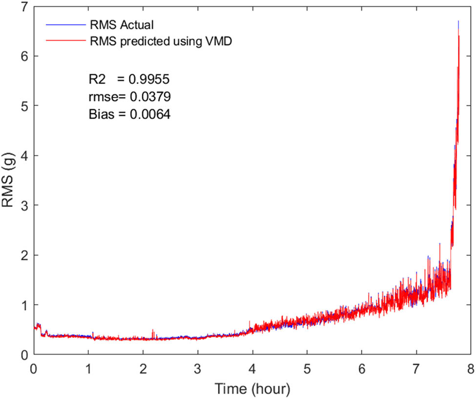
RMS over time for original signals and denoised signals.

3.2 Construction of DT

To build a DT, the following steps are taken as shown in Figure 9:

collection and processing of vibration signals,
define a list of features and decisions, then build the data set using the Weka software, and
the data set is subjected to the J48 classification algorithm in order to create a DT and get knowledge from it.

Figure 9

Features and decisions.

In this study, two data set were constructed. The first data set is based on original vibration signals, and the second is based on denoised vibration signals. Using the J48 classifier algorithm on the data set allowed us to build the DTs shown in Figures 10 and 11, which correspond to noised and denoised signals, respectively. Figure 10, which corresponds to the original vibration signals, demonstrates that the most significant features to evaluate throughout the monitoring process are RMS and RA.

Figure 10

DT from original vibration signals.

Figure 11

DT from denoised vibration signals.

On the other hand, Figure 11, which corresponds to the denoised vibration signals, shows that the most important features to consider during the monitoring process are RMS and RANGE (Table 2). Furthermore, the RMS feature appears to be more reliable than the other features for monitoring the fault.

The number of correctly classified samples can be found in the diagonal elements of the confusion matrix for the original and denoised signals, as shown in Tables 3 and 4. The elements on the outer diagonal, on the other hand, represent the number of samples that were classified incorrectly using the DT method.

Table 3

Confusion matrix correspondent to original signals

Classified as →	Normal	Abnormal	Danger
Normal	1,616	35	0
Abnormal	49	1,060	0
Danger	0	4	39

Table 4

Confusion matrix correspondent to denoised signals

Classified as →	Normal	Abnormal	Danger
Normal	1,612	37	0
Abnormal	68	1,043	0
Danger	0	4	39

Classification rates ranged from 96.11 to 96.86 , with kappa statistics ranging 0.92 – 0.93 , as shown in Table 5. It is essential to recognize that a rate of classification of 1 denotes excellent modeling, and a kappa statistic of 0.7 or above denotes good statistics correlation.

Table 5

The DT’s performance

	Original signals	Denoised signals
Classification rate	96.86	96.11
Kappa statistic	0.93	0.92
Mean absolute error	0.04	0.05
Root mean square error	0.14	0.16
Number of samples	2,803	2,803
Number of leaves	4	3
Size of the tree	8	5

Although the results of the two trees are similar, we notice a difference in the characteristics of each tree on which they rely for decision-making. This difference is due to how the signals are processed.

3.3 RUL estimation by ELM

Several improved versions of the basic ELM have recently been developed to solve regression and classification problems. Interested readers are referred to references [37,43], which survey ELM and its variants.

The ELM technique is used in this part to build a nonlinear relationship between features collected from vibration signals and the RUL of ball bearings. Table 6 summarizes the details of the parameters and performance of ELM. The RUL obtained by applying the ELM algorithm on the two independent data sets formed from original and denoised signals is shown in Figures 12 and 13. The effect of the number of hidden neurons and the features of the DTs in RUL modeling is clearly shown.

Table 6

Performances of ELM

	Original signals	Denoised signals
R Squared	1.0	1.0
Number of hidden neurons (NHN)	3,500	5,700
Neural transfer function	Triangular basis	Triangular basis
Input	RMS, RA	RMS, RANGE

Figure 12

RUL Prediction based on original vibration signals.

Figure 13

RUL Prediction based on denoised vibration signals.

4 Conclusions

In this research article, a novel approach to condition monitoring was presented, utilizing VMD, DT, and ELM algorithms. The VMD algorithm was first used to reduce noise in the original vibration signals, followed by the application of the J48 algorithm to both signals, namely the actual and the one processed with VMD. Finally, the ELM algorithm was used to estimate the RUL of the monitored system. The results of this study demonstrate that this methodology provides highly accurate RUL prediction, allowing for the health monitoring of ball bearings and RUL estimation based on multiple features rather than relying solely on the RMS feature as done in many previous studies. The proposed methodology therefore has the potential to be highly beneficial in the decision-making process for condition monitoring applications. Overall, this research presents a promising new methodology for accurate and efficient condition monitoring.

Funding information: The authors state no funding involved.
Author contributions: All authors have accepted responsibility for the entire content of this manuscript and approved its submission.
Conflict of interest: The authors state no conflict of interest.

References

[1] Jardine AK, Lin D, Banjevic D. A review on machinery diagnostics and prognostics implementing condition-based maintenance. Mech Syst Signal Process. 2006;20(7):1483–510. 10.1016/j.ymssp.2005.09.012.Search in Google Scholar

[2] Lee J, Abujamra R, Jardine AK, Lin D, Banjevic D. An integrated platform for diagnostics, prognostics and maintenance optimization. Proceedings of the Intelligent Maintenance Systems; 2004 Jul 15. p. 15–27.Search in Google Scholar

[3] Boumahdi M, Rechak S, Hanini S. Analysis and prediction of defect size and remaining useful life of thrust ball bearings: modelling and experiment procedures. Arab J Sci Eng. 2017;42(11):4535–46. 10.1007/s13369-017-2550-y.Search in Google Scholar

[4] Soualhi A, Medjaher K, Zerhouni N. Bearing health monitoring based on Hilbert–Huang transform, support vector machine, and regression. IEEE Trans Instrum Meas. 2014;64(1):52–62. 10.1109/TIM.2014.2330494.Search in Google Scholar

[5] Benkedjouh T, Medjaher K, Zerhouni N, Rechak S. Remaining useful life estimation based on nonlinear feature reduction and support vector regression. Eng Appl Artif Intell. 2013;26(7):1751–60. 10.1016/j.engappai.2013.02.006.Search in Google Scholar

[6] Yan M, Wang X, Wang B, Chang M, Muhammad I. Bearing remaining useful life prediction using support vector machine and hybrid degradation tracking model. ISA Trans. 2020;98:471–82. 10.1016/j.isatra.2019.08.058.Search in Google Scholar PubMed

[7] Ambrosino F, Thinová L, Briestenský M, Šebela S, Sabbarese C. Detecting time series anomalies using hybrid methods applied to Radon signals recorded in caves for possible correlation with earthquakes. Acta Geodaetica et Geophysica. 2020;55:405–20. 10.1007/s40328-020-00298-1.Search in Google Scholar

[8] Mao W, He J, Li Y, Yan Y. Bearing fault diagnosis with auto-encoder extreme learning machine: A comparative study. Proc Inst Mech Engineers, Part C: J Mech Eng Sci. 2017;231(8):1560–78. 10.1177/0954406216675896.Search in Google Scholar

[9] Lee J, Sun Z, Tan TB, Mendez J, Flores-Cerrillo J, Wang J, et al. Remaining useful life estimation for ball bearings using feature engineering and extreme learning machine. IFAC-PapersOnLine. 2022;55(7):198–203. 10.1016/j.ifacol.2022.07.444.Search in Google Scholar

[10] Mao W, He L, Yan Y, Wang J. Online sequential prediction of bearings imbalanced fault diagnosis by extreme learning machine. Mech Syst Signal Process. 2017;83:450–73. 10.1016/j.ymssp.2016.06.024.Search in Google Scholar

[11] Wu Y, Yuan M, Dong S, Lin L, Liu Y. Remaining useful life estimation of engineered systems using vanilla LSTM neural networks. Neurocomputing. 2018;275:167–79. 10.1016/j.neucom.2017.05.063.Search in Google Scholar

[12] Ren L, Sun Y, Wang H, Zhang L. Prediction of bearing remaining useful life with deep convolution neural network. IEEE Access. 2018;6:13041–49. 10.1109/ACCESS.2018.2804930.Search in Google Scholar

[13] Chen Y, Peng G, Zhu Z, Li S. A novel deep learning method based on attention mechanism for bearing remaining useful life prediction. Appl Soft Comput. 2020;86:105919. 10.1016/j.asoc.2019.105919.Search in Google Scholar

[14] Gupta M, Wadhvani R, Rasool A. A real-time adaptive model for bearing fault classification and remaining useful life estimation using deep neural network. Knowl Syst. 2023;259:110070. 10.1016/j.knosys.2022.110070.Search in Google Scholar

[15] Ambrosino F, Sabbarese C, Roca V, Giudicepietro F, Chiodini G. Analysis of 7-years Radon time series at Campi Flegrei area (Naples, Italy) using artificial neural network method. Appl Radiat Isotopes. 2020;163:109239. 10.1016/j.apradiso.2020.109239.Search in Google Scholar PubMed

[16] Santosh T, Soni RK, Eswaraiah C, Kumar S. Application of artificial neural network method to predict the breakage properties of PGE bearing chromite ore. Adv Powder Technol. 2022;33(3):103450. 10.1016/j.apt.2022.103450.Search in Google Scholar

[17] Peng F, Zheng L, Peng Y, Fang C, Meng X. Digital Twin for rolling bearings: a review of current simulation and PHM techniques. Measurement. 2022;201:111728. 10.1016/j.measurement.2022.111728.Search in Google Scholar

[18] Xu Z, Saleh JH. Machine learning for reliability engineering and safety applications: Review of current status and future opportunities. Reliab Eng & Syst Saf. 2021;211:107530. 10.1016/j.ress.2021.107530.Search in Google Scholar

[19] Bertolini M, Mezzogori D, Neroni M, Zammori F. Machine learning for industrial applications: A comprehensive literature review. Expert Syst Appl. 2021;175:114820. 10.1016/j.eswa.2021.114820.Search in Google Scholar

[20] Soni D, Kumar N. Machine learning techniques in emerging cloud computing integrated paradigms: A survey and taxonomy. J Netw Comput Appl. 2022;205:103419. 10.1016/j.jnca.2022.103419.Search in Google Scholar

[21] Avci O, Abdeljaber O, Kiranyaz S, Hussein M, Gabbouj M, Inman DJ. A review of vibration-based damage detection in civil structures: From traditional methods to machine learning and deep learning applications. Mech Syst Signal Process. 2021;147:107077. 10.1016/j.ymssp.2020.107077.Search in Google Scholar

[22] Li X, Liu X, Yue C, Liang SY, Wang L. Systematic review on tool breakage monitoring techniques in machining operations. Int J Mach Tools Manufacture. 2022;103882. 10.1016/j.ijmachtools.2022.103882.Search in Google Scholar

[23] Ntemi M, Paraschos S, Karakostas A, Gialampoukidis I, Vrochidis S, Kompatsiaris I. Infrastructure monitoring and quality diagnosis in CNC machining: A review. CIRP J Manuf Sci Technol. 2022;38:631–49. 10.1016/j.cirpj.2022.06.001.Search in Google Scholar

[24] van Dinter R, Tekinerdogan B, Catal C. Predictive maintenance using digital twins: A systematic literature review. Inf Softw Technol. 2022;151:107008. 10.1016/j.infsof.2022.107008.Search in Google Scholar

[25] Zhao R, Yan R, Chen Z, Mao K, Wang P, Gao RX. Deep learning and its applications to machine health monitoring. Mech Syst Signal Process. 2019;115:213–37. 10.1016/j.ymssp.2018.05.050.Search in Google Scholar

[26] Gangsar P, Tiwari R. Signal based condition monitoring techniques for fault detection and diagnosis of induction motors: A state-of-the-art review. Mech Syst signal Process. 2020;144:106908. 10.1016/j.ymssp.2020.106908.Search in Google Scholar

[27] Hakim M, Omran AAB, Ahmed AN, Al-Waily M, Abdellatif A. A systematic review of rolling bearing fault diagnoses based on deep learning and transfer learning: Taxonomy, overview, application, open challenges, weaknesses and recommendations. Ain Shams Eng J. 2022;14:101945. 10.1016/j.asej.2022.101945.Search in Google Scholar

[28] Huang HZ, Wang HK, Li YF, Zhang L, Liu Z. Support vector machine-based estimation of remaining useful life: current research status and future trends. J Mech Sci Technol. 2015;29(1):151–63. 10.1007/s12206-014-1222-z.Search in Google Scholar

[29] Liu H, Mo Z, Zhang H, Zeng X, Wang J, Miao Q. Investigation on rolling bearing remaining useful life prediction: A review. In 2018 Prognostics and System Health Management Conference (PHM-Chongqing) (pp. 979-984). IEEE; 2018, October. 10.1109/PHM-Chongqing.2018.00175.Search in Google Scholar

[30] Si XS, Wang W, Hu CH, Zhou DH. Remaining useful life estimation–a review on the statistical data driven approaches. Eur J Oper Res. 2011;213(1):1–14. 10.1016/j.ejor.2010.11.018.Search in Google Scholar

[31] Huang Y, Lin J, Liu Z, Wu W. A modified scale-space guiding variational mode decomposition for high-speed railway bearing fault diagnosis. J Sound Vibratio. 2019;444:216–34. 10.1016/j.jsv.2018.12.033.Search in Google Scholar

[32] Boumahdi M, Dron JP, Rechak S, Cousinard O. On the extraction of rules in the identification of bearing defects in rotating machinery using decision tree. Expert Syst Appl. 2010;37(8):5887–94. 10.1016/j.eswa.2010.02.017.Search in Google Scholar

[33] Breiman L, Friedman JH, Olshen RA, Stone CJ. Classification and regression trees. technical report. Belmont, CA: Wadsworth International Group; 1984.Search in Google Scholar

[34] Quinlan JR. Induction of decision trees. Mach Learn. 1986;1(1):81–106.10.1007/BF00116251Search in Google Scholar

[35] Quinlan JR. C4.5: Programs for machine learning. Mach Learn. Vol. 16. Morgan Kaufmann Publishers; 1993. p. 235–40.10.1007/BF00993309Search in Google Scholar

[36] Huang GB, Zhu QY, Siew CK. Extreme learning machine: theory and applications. Neurocomputing. 2006;70(1–3):489–501. 10.1016/J.NEUCOM.2005.12.126.Search in Google Scholar

[37] Ding S, Xu X, Nie R. Extreme learning machine and its applications. Neural Comput Appl. 2014;25(3):549–56. 10.1007/s00521-013-1522-8.Search in Google Scholar

[38] Sureka N, Gunaseelan K. Investigations on detection and prevention of primary user emulation attack in cognitive radio networks using extreme machine learning algorithm. J Ambient Intell Humanized Comput. 2021;1–10. 10.1007/s12652-021-03080-5.Search in Google Scholar

[39] Nectoux P, Gouriveau R, Medjaher K, Ramasso E, Chebel-Morello B, Zerhouni N, et al. PRONOSTIA: An experimental platform for bearings accelerated degradation tests. IEEE International Conference on Prognostics and Health Management, PHM’12., Jun 2012. Denver, Colorado, United States; 2012, June; p. 1–8. HAL Id: hal-00719503. https://hal.archives-ouvertes.fr/hal-00719503.Search in Google Scholar

[40] Wang L, Zhang L, Wang XZ. Reliability estimation and remaining useful lifetime prediction for bearing based on proportional hazard model. J Cent South Univ. 2015;22(12):4625–33. 10.1007/s11771-015-3013-9.Search in Google Scholar

[41] Euldji R, Boumahdi M, Bachene M. Decision-making based on decision tree for ball bearing monitoring. 2020 2nd Int Workshop Human-Centric Smart EnvirHealth Well-being (IHSH). IEEE; 2021, Febr. p. 171–5. 10.1109/IHSH51661.2021.9378734.Search in Google Scholar

[42] Isham MF, Leong MS, Lim MH, Ahmad ZA. Variational mode decomposition: mode determination method for rotating machinery diagnosis. J Vibroengineering. 2018;20(7):2604–21. 10.21595/jve.2018.19479.Search in Google Scholar

[43] Huang GB, Wang DH, Lan Y. Extreme learning machines: a survey. Int J Mach Learn Cybern. 2011;2(2):107–22. 10.1007/s13042-011-0019-y.Search in Google Scholar

Received: 2023-01-14

Revised: 2023-02-23

Accepted: 2023-02-24

Published Online: 2023-06-12

This work is licensed under the Creative Commons Attribution 4.0 International License.

Articles in the same Issue

https://doi.org/10.1515/phys-2022-0239

Keywords for this article

condition monitoring; ball bearings; variational mode decomposition; decision tree; extreme learning machines

Creative Commons

BY 4.0