Behaviour and onset of low-dimensional chaos with a periodically varying loss in single-mode homogeneously broadened laser

1 Introduction

The single-mode unidirectional ring laser containing a homogeneously broadened medium with two-level atoms [1,2], and the Lorenz model that describes fluid turbulence [3, 4,5,6, 7,8,9], both known for leading to deterministic chaos, are isomorphic to each other, as demonstrated by Haken [10]. This simplest model of laser, so-called the Lorenz–Haken model, can be viewed as a system, which becomes unstable under suitable conditions related to the respective values of the decay rates (bad cavity condition) and to the level of excitation (second laser threshold) [11]. The numerical and analytical studies [12,13, 14,15,16, 17,18] of the Lorenz–Haken model have displayed that the system undergoes a transition from a stable continuous wave output to a regular pulsing state (pulsations may be periodic or period doubled). However it can also develop irregular oscillations (chaotic solutions). The nature of such irregular solutions was explained by Haken [10,19]. The previous numerical studies by Nadurcci et al. [16] revealed the existence of domain of values of the laser parameter, below the second laser threshold 2 C 2 th , in which periodic or chaotic solutions cohabit with the locally stable stationary state. This region of parameter space is called the hard excitation domain, because the oscillating solutions can only be produced following a sufficiently large disturbance of the stable stationary state. In Section 2, we re-examine the behaviour of the single-mode laser equations above and below the second laser threshold, versus a hard excitation and versus an infinitesimal perturbation of the steady state, for the values of the atomic decay rates and relaxation rates of the laser field referred in previous publications [12,13, 14,15]. Coexisting periodic or chaotic oscillations (hard excitation) with stationary solutions (infinitesimal perturbation) develop when the ration ℘ of the population ( ℘ ‖ ) over the polarisation decay rate ( ℘ ⊥ ) is sufficiently smaller than ℘ = 1.0 . Chaotic solution and stationary states coexist for values of ℘ greater than approximately 0.11, before reaching the critical value. This values ℘ = 0.11 has been analytically predicted by our analytical approach [15]. Below and in the vicinity of the second laser threshold, for ℘ smaller than 0.11, periodic solutions and chaotic oscillations cohabit with the stable stationary state. Increasing the pump parameter beyond the second laser threshold for ℘ smaller than 0.11, the oscillations remain periodic versus hard and infinitesimal perturbation. In this region defined by ℘ < 0.11 , the Lorenz–Haken system has a periodic behaviour because the characteristic pumping rate 2 C P [14] is greater than or close to the second laser threshold 2 C 2 th . Chaotic oscillations develop for higher values of the pump parameter. We show in Section 3 that introducing an adiabatic elimination of the polarisation with a periodically varying loss, the single-mode homogenously broadened laser can exhibit chaotic emission if the frequency ω is near to the natural frequency Δ P [14,15]. In Section 4, we propose a reformulation of the analytical approach applied in the previous works [12,13, 14,15], by adding a phase terms to the electric-field expansion, and demonstrate that the asymmetric aspect that appears in the time evolution of the electric field is due to the phase effects between the electric field components.

2 Hard and small perturbation above and below the second laser threshold

The semiclassical model for a single-mode, homogenously broadened laser is the simplest model, which exhibits the pulsation behaviour here of interest. This model has also been the most widely studied. The derivation of the differential equations governing this basic model is widely available and is omitted here for brevity. The popular semiclassical models for homogeneously broadened lasers differ mainly in notation and normalisation. The model adopted in this work is based on the Maxwell–Bloch equations in single-mode approximation, for a unidirectional ring laser containing a homogeneously broadened medium [16,17]. The equations of motion are obtained using a semi-classical approach, considering the resonant field inside the laser cavity as a macroscopic variable interacting with a two-level system. Assuming exact resonance between the atomic line and the cavity mode, and after adequate approximations, one obtains three differential non-linear coupled equations for the field, polarisation, and population inversion of the medium, the so-called Lorenz–Haken model:

where P ( t ) represents the atomic polarisation, E ( t ) is the electric field in the laser cavity having a decay constant κ , D ( t ) is the population difference having a decay constant ℘ , and both κ and ℘ are scaled to the polarisation relaxation rate ( ℘ ⊥ ). The term 2 C denotes the pump rate required for reaching the lasing effect ( 2 C = 1 ). It is normalised to have a value of unity at the threshold for laser action ( 2 C 1 t h = 1 ). These equations are actually typical of all laser instability models, in the sense that they are a set of coupled first-order non-linear differential equations governing the time dependence of the laser parameters. The most familiar type of stability criteria concerns the smallest value of the threshold parameter 2 C for which an infinitesimal perturbation of the steady state will lead to a divergence from this steady state. Such a criterion may be obtained using the linear stability analysis [13,11]. For the model represented by Eq. (1), this criterion can be obtained analytically, and the well-known result is [14]:

provided that κ > 1 + ℘ . This expression shows dependence to the parameters ℘ and κ and indicates that the pumping rate 2 C 2 th increases with increasing parameter ℘ for a given κ . Eq. (1) have two fixed points, i.e., three stationary solutions given by:

The two solutions (Eq. (4)) correspond to the same stationary state intensity:

The linear stability analysis indicates that the steady-state solutions (Eq. (4)) are stable against the growth of an infinitesimal perturbation in the range 1 < 2 C < 2 C 2 th , whereas for 2 C > 2 C 2 th , any perturbation of the steady-state solutions (Eq. (4)) would inevitably grow. This growth indicates that for these 2 C > 2 C 2 th values, steady-state laser operation is impossible. As is well known [11], at the critical value 2 C 2 th , the solution undergoes a subcritical Hopf bifurcation [11] and loses stability to a large amplitude pulsing solution [11,16,17]. The optimum value of κ that minimizes the threshold instability (Eq. (2)) of the steady-state solutions is given by:

This is in the range 3 < κ < 5 for ℘ in the range 0 < ℘ < 1 .

In previous works [12,13,14], a simple harmonic expansion method that yields to analytical solutions for the laser equations has been derived. We have demonstrated that the inclusion of the third-order harmonic term in the field expansion allows for the prediction of the pulsing frequency Δ P of the regular pulse trains expressed by [14,15]:

It constitutes an expression of the natural frequency that characterizes a given set of κ and ℘ values that allows for periodic solutions. This frequency delimits a zone where the laser exhibits regular oscillations for the values of the parameter pumping 2C greater than the critical value 2 C 2 th [15]. We have also revealed the tendency of the dissipative Lorenz–Haken system to behave periodic for a characteristic pumping rate 2 C p [14]. In this section, we re-examine the behaviour of Lorenz–Haken system under small and hard excitation. We consider fixed value of κ = 3.0 (the value that minimizes the threshold instability), which has already been used in preceding works [12,13, 14,15], and a pump parameter varying from 0 to 25. The solid line in Figure 1 denotes the instability threshold 2 C 2 th versus the parameter ℘ scanned over the 0 < ℘ < 1 range. We apply the same analytical procedure that has been described in references [12,13, 14,15] to delimit the boundary region between chaotic and periodic solutions. The dotted line at the right of the curve 2 C 2 th in Figure 1 displays this region limit. The periodic solutions are limited to ℘ ≤ 0.11 [15].

Figure 1

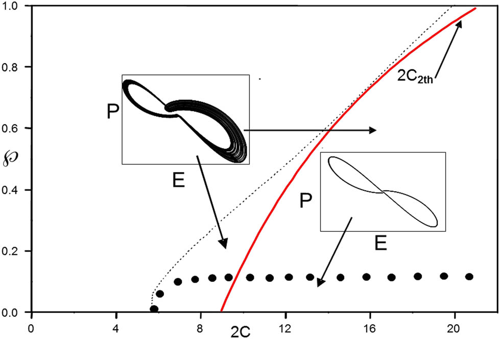
Stability boundaries for a homogenously broadened laser as function of the threshold parameter 2 C and the decay rate ℘ for a laser satisfying κ = 3 . The solid curve represents the second laser threshold 2 C 2 th for which an infinitesimal perturbation of the steady-state will lead to a divergence from this steady state. The broken curve denotes the end of the large perturbation (hard excitation) domain. The dotted line represents the frontier between chaotic states and periodic solutions (below this dotted line).

The physical description of the appearance of the periodic behaviour is that in this region of the dissipative Lorenz–Haken system ( ℘ ≤ 0.11 ), the characteristic pumping rate [14]:

is greater than or equal to the second laser threshold 2 C 2 th . This formula shows dependence to the parameter ℘ for a given κ and indicates that the pumping rate 2 C P decreases with the increasing parameter ℘ . With ℘ = 0.1 and κ = 3.0 , we obtain 2 C P = 9.79 (Eq. (8)) and 2 C 2 th = 9.63 (Eq. (2)), the value of 2 C P being therefore greater than the value 2 C 2 th . A sample of the corresponding phase space projection of these regular solutions is also shown in this domain (Figure 1). As expected, there is a close agreement between those results derived from the analytical approach [15] and the results obtained by numerical integration of Eq. (1), using a Runge–Kutta method with an adaptive integration step. The numerical calculations reveal that this region of periodic oscillations arises, even from an infinitesimal perturbation and also against a large amplitude perturbation of the steady-state solutions, Eq. (4). On the contrary, regular and irregular pulsating solutions occur only following a large amplitude perturbation of the steady solutions Eq. (4), for the region of the parameter pumping 2 C < 2 C 2 th (at the left of the curve 2 C 2 th in Figure 1). In this zone, the steady-state solutions are stable against small perturbations and unstable against a large perturbation. This region is called hard excitation domain. The dotted line in Figure 1, at the left of 2 C 2 th and for ℘ ≤ 0.11 , marks a periodic region not predicted by the linear stability analysis. On the other hand, this region is well predicated by our analytical approach [15]. In this domain, periodic solutions cohabit with the stable stationary state. This periodic behaviour is due to the fact that in the region ℘ ≤ 0.11 , the characteristic pumping rate 2 C P is greater than the second laser threshold 2 C 2 th . The broken line to the left of the laser threshold in Figure 1 indicates the boundary of the “hard excitation domain” obtained by a numerical integration of Eq. (1). In this zone, chaotic pulsations emerge for ℘ > 0.11 and coexist with the stable stationary state. We have included the projection of the Lorenz attractor along the population inversion axis of the phase for ℘ > 0.1 and for 2 C < 2 C 2 th in Figure 1. The physical interpretation of the abrupt appearance of chaotic behaviour is that in this region ( ℘ > 0.11 ), the pumping rate 2 C P (Eq. (8)) required to have periodic oscillations is smaller than the critical value 2 C 2 th . So, it is difficult to have periodic solutions. For example, with ℘ = 0.15 and κ = 3.0 , we obtain 2 C P = 7.27 from Eq. (8) and 2 C 2 th = 9.97 from Eq. (2), and therefore, the value of 2 C P is here smaller than the value 2 C 2 th . The existence of a hard excitation domain indicates coexistence of time-dependent and steady-state solutions and points to the appearance of hysteresis behaviour in adiabatic gain scans [11,16].

Figure 2 then depicts the bifurcation diagram constructed with a fixed values κ = 3.0 , ℘ = 0.1 , and for 2 C varying within the 1 < 2 C < 32 range, and under small perturbation (Figure 2(a)) and large perturbation (Figure 2(b)). In the case of small perturbation (Figure 2(a)), and for 2 C greater than 2 C 2 th = 9.63 , a periodic doubling sequence is observed, first leading to chaotic behaviour for 2 C ≥ 32 . The periodic solutions may be of the period symmetric or asymmetric type [15,16]. However, the steady-state solutions are stable for 2 C < 2 C 2 th = 9.63 . In the case of large perturbation (Figure 2(b)), the steady-state solutions are stable for 2 C < 6.11 . For 2 C in the 6.11 < 2 C < 7 range, a chaotic behaviour is observed. For 2 C > 7 , the solutions may be of the period symmetric or asymmetric type. Finally, a chaotic behaviour appears again for 2 C ≥ 32 .

Figure 2

Nature of the solutions of Eq. (1) with (a) small perturbation and (b) large perturbation, constructed with a fixed values κ = 3 and ℘ = 0.1 while 2 C varies in the range 0 < 2 C < 32 .

Note that stability versus chaos investigations can also be performed by computing Lyapunov’s exponent λ [20,21,22] to quantify the sensitivity to initial conditions, in order to distinguish chaotic behaviour from predictable one. If real part of λ is positive, the sensitivity to the initial conditions is very high, and if imaginary part of λ is negative the solution is stable. This is the linear stability analysis called small perturbation. In the case of the so-called hard perturbation, the system is allowed to evolve from two distant initial conditions, and it is observed whether the two trajectories merge. Note that a hysteresis or bistability phenomenon can also appear. In the hard excitation domain, for 2 C < 2 C 2 th region, with ℘ < 0.11 , the periodic solution (large perturbation) and the steady state coexist, and with ℘ > 0.11 , the chaotic solution (large perturbation) coexists with the steady state. This region of the parameter is called hard excitation domain because oscillating solutions (periodic or chaotic) can only be produced versus a large perturbation ( X s + x ) of the stationary state X s locally stable. For ℘ < 0.11 , the average intensity ⟨ E ( t ) 2 ⟩ of the periodic oscillations is less than the stationary value E s 2 (Figure 3(a)). The average values of the energy of the system lie along a straight line parallel to that of the energy of the system in the stationary state, this refers for 2 C < 2 C 2 th to the hysteresis phenomenon or bistability, where two attractors can coexist: the stationary solution represented by a fixed point in phase space and the periodic solution represented by a limit cycle in the phase space. Finally, the chaotic signal can be identified by an easy method, leading to same conclusion as the Lyapunov exponent, by computing the FFT of the signal. The frequency spectrum of a chaotic regime is wide and a strange attractor in phase space emerges. In particular, a system is chaotic if its spectrum includes a continuous component, independently of the possible presence of a few peaks. For example, for ℘ = 0.2 , k = 3.0 and 2 C = 2 C 2 th − 1 = 9.33 − 1 = 8.33 , one obtains Figure 3(b) and (c) for the strange attractor and frequency spectrum, in this case depicting a chaotic regime. However, in the periodic and quasi-periodic regimes, we observe a cycle limit and a torus, respectively, in the phase portrait, and the frequency spectrum in the quasi-periodic regime includes frequency components in irrational relationship [23,24,25].

Figure 3

(a) In the hard excitation domain, for 2 C < 2 C 2 th region, with ℘ < 0.11 , the average intensity ⟨ E ( t ) 2 ⟩ of periodic oscillations is smaller than the stationary value E s 2 . (b) Strange attractor appearing for ℘ = 0.2 and κ = 3 and 2 C < 2 C 2 th − 1 = 9.33 − 1 = 8.33 , 2 C < 2 C 2 th . (c) Corresponding continuous frequency spectrum, characteristic of the chaotic behaviour.

3 Adiabatic elimination: chaos with low dimension

For the single-mode homogenously broadened laser described by Eq. (1), the adiabatic elimination of the polarisation [26,27,28] excludes the possibility of even periodic solutions, only transient relaxation oscillations are possible, and then only if the population decay rate ℘ ‖ is smaller than the field decay rate κ [29]. The dynamics is ruled by two rate equations for the electric field and the population inversion. In general, when there are two dynamical variables, the system can have either constant or period solutions, whereas at least three variables (degrees of freedom) are needed to observe chaotic behaviour. With ℘ ⊥ » κ , ℘ ‖ , the polarisation undergoing fast-decay processes is in dynamical equilibrium with the electric field and population inversion that evolve at a much slower rate. Furthermore, we can eliminate the fast variable (polarisation) adiabatically. The adiabatic elimination process imposes limitations on the possible emergence of pulsations or chaos. In this situation, only relaxation oscillations can be observed during the transient approach to steady state. The existence of this resonance has been cleverly exploited to achieve regular pulsating by matching the modulation frequency of the resonator losses to the characteristic frequency, determined by a linear stability analysis. With lower amplitude modulation, one can obtain a period-doubling, quasi-periodic, and chaotic behaviour. First quantitative evidence of chaos in a modulated loss CO 2 laser was given in refs [26,28]. In this section, we study the dynamic behaviour of the laser being in class B [26] with periodically varying loss. The dynamics is ruled only by two rate equations, namely:

and with:

This yield to:

Injecting the aforementioned expression in the system Eq. (9) with the field intensity I = E 2 , one obtains the following system that describes the dynamic behaviour of laser being in class B:

In order to introduce a third dynamic variable necessary for chaos emergence, we resort to periodically varying losses. We assume a sinusoidal time-dependent perturbation of the cavity rate κ as follows:

where ω is the frequency set around Δ P (Eq. (7)). We choose Δ P because this frequency constitutes an expression of the natural frequency that characterizes a given set of κ and ℘ . The terms a and á are the dc component and the amplitude of the cavity rate κ , respectively. The term κ 0 represents the unperturbed cavity relaxation rate. If ω is close to Δ P , non-linear resonances are excited and the laser can exhibit chaotic emission.

The value of the amplitude á must be greater than 1 because the natural frequency Δ P characterizes the strong oscillations around zero of the Lorenz–Haken system [12,13,14].

On the contrary, if ω is far from the frequency Δ P , the system displays a steady-state laser operation or follows the sinusoidal variation of κ . Numerical simulations with fixed modulation frequency and amplitude ω = Δ P , a = 1 and á = 1.5 for typical parameter ℘ = 0.004 and κ 0 = 0.1 have been performed, and a period doubling cascade T, 2T, 4T, 8T, and chaos is observed, providing a well-reproduced Feigenbaum’s scenario [30]. Figure 4 shows the behaviour of these periodic solutions when increasing pumping parameter 2 C . First, the laser displays a solution with period one, Figure 4(a). The projection of the trajectory onto the (I,D) plane produces loop as shown in Figure 4(b). Increasing the excitation level 2 C ( 2 C = 3.10 ), the laser exhibits a solution with period-two, Figure 4(c). This feature corresponds to the two-loop periodic solution, Figure 4(d). As the excitation level further increases, the laser exhibits a solution with period four for 2 C = 3.12 as shown in Figure 4(e) (four-loop periodic solution, Figure 4(f)) and then, a solution with period eight with 2 C = 3.14 , depicted in Figure 4(g) (eight-loop periodic solution, Figure 4(h)). This cascade eventually leads to chaotic behaviour shown in Figures 4(i) and (j).

Figure 4

Examples of system Eq. (12) solutions with sinusoidal time-dependent perturbation of the cavity rate κ for κ 0 = 0.1 , ℘ = 0.004 , a’ = 1.5, and ω = Δ P . The left hand figure is the time dependence of the electric field Intensity. (a) Solution with period-one, obtained with 2 C = 3.0 . (c) Solution with period two, obtained with 2 C = 3.10 . (e) Solution with period-four, obtained with 2 C = 3.12 . (g) Solution with period-eight, obtained with 2 C = 3.14 . (i) Chaotic solution obtained with 2 C = 3.2 . The right-hand figures (b,d,f,h,j) corresponding attractor projections onto the (I,D) plane. A cascade of period doubling is observed, which finally leads to chaotic behaviour.

4 Analytical solutions with an additional phase terms to the electric-field expansion

The strong and simple harmonic expansion applied in the previous works [12,13,14] permit to derive an analytical solution for the Lorenz–Haken equations. This approach describes the physical situations where the long-term signal consists in regular pulse trains (periodic solutions). The corresponding laser field and polarisation oscillate around a zero mean-value and the corresponding frequency spectra exhibit odd-order components of the fundamental pulsating frequencies Δ P , while the population inversion oscillates with a dc component and population inversion spectrum exhibits even components [12,13,14]. This analytical procedure has allowed deriving the amplitude of the first-, third-, fifth- and the seven-order harmonics for the laser-field expansion [15]. We have shown that this iterative method is limited to the third order, and that above, the obtained analytical solution diverges from the numerical direct resolution of the equations [15].

As pointed out by one of the referees, the use of non-convergent methods can be quite dangerous, as there is always a possibility to obtain unreliable results. As such, the here-proposed method is not of general validity for any range of pumping, population inversion etc …, but its validity was acquired for the typical values previously considered [12,13,14]. In more general cases, the results obtained with this method should be confirmed by numerical simulations.

In particular, we have shown using a typical example that the inclusion of the third-order harmonic term in the field expansion allows for the prediction of the pulsing frequency [12,13,14]:

This analytical expression of pulsing frequencies excellently matches their numerical counterparts [15]. In the proposed analytical expansions:

and

we have supposed a phase locking between all the terms that appear in the electric-field expansion, Eq. (15a), and have ignored the dephasing process that takes place between the terms in this expansion. However, for the polarisation and population, we have taken into account the in-phase (P 2 n + 1 , D 2 n + 1 ) and out-phase (P 2 n + 2 , D 2 n + 2 ) components in expressions Eqs. (15b) and (15c). The time evolution of the analytical electric field (Eq. (15a)) illustrated in Figure 5(a) cannot describe the asymmetry of E ( t ) with respect to E = 0 (Figure 5(b)) obtained by numerical integration of Eq. (1) with 2 C = 16 , κ = 3 and ℘ = 0.1. This asymmetric feature, which increases with the excitation pump 2 C , is due to the phase effects between the electric field components. In this work, we propose a reformulation of the analytical approach by adding a phase terms to the electric-field expansion Eq. (15a), in order to derive electric field amplitude and phase expressions in the case of symmetric phase-space portrait [15]. The asymmetric phase-space portrait appearing for 2 C > 18.4 has been studied in ref. [31] without taking into account the phase terms in the electric-field expansion.

Figure 5

(a) Analytical solutions representation for the electric-field expansion, Eq. (15a), up to the third-order without the dephasing process. (b) Long-term time dependence of the electric-field obtained by numerical integration of Eq. (1). (c) Analytical solutions representation for the electric-field expansion, Eq. (21), up to the third-order and with the dephasing process taken into account, and for κ = 3 , ℘ = 0.1 , and 2 C = 16 . The asymmetric feature of E ( t ) with respect to E = 0 is due to the phase effects between the electric field components.

Therefore, the new analytical development is:

Limiting these expansions to the third order for the field and polarisation, and to the second order for the population inversion in Eq. (16), we obtain:

The first-order field amplitude in Eq. (15a) serves as references with respect to higher order components ( φ 1 = 0 and φ 3 = φ ). The evaluation of the in-phase E 3 s and the out-phase E 3 c amplitudes suggests using the mathematical identity:

Injecting this identity into the expansion Eq. (17a), one obtain:

We apply here the same procedure described in ref. [32] to obtain the analytical expression of the phase appearing in the expression of the inversion population D ( t ) (Eq. (19c)):

where

Inserting the aforementioned expansions into Eq. (1) and equalising terms of the same order in each relations yield to a system of algebraic relations between the various amplitudes. Solving this system using the Mathematica software, we found an analytical expression of the ration E 3 s / E 3 c between the out-phase and in-phase third-order, as follows:

and this expression is related to the decay rates ℘ and κ , and to the excitation parameter 2 C through their dependence on the pulsing frequency Δ , Eq. (14). Taking into account that, one obtains the following analytical expression of the electric field that evolves according to:

where

and with:

We can now construct a typical sequence of analytical solutions. The long-term operating frequency is estimated from Eq. (14), while the first- and third-order field components are evaluated from Eqs. (25) and (24), respectively, the phase being evaluated from Eq. (22). The values of these components, for κ = 3 , ℘ = 0.1 and 2 C = 16 , are E 1 = 8.31 and E 3 = 3.02 and the corresponding frequency is Δ = 0.55 with the phase φ = 0.03 . Thus, to third order, the analytical field expansion takes the following expression:

The temporal evolution of Eq. (26) is illustrated in Figure 5(c). One may conclude that the asymmetric aspect is due to the phase effects between the electric field components. However, differences remain between the analytical and the numerical solutions. The pulses peak at E N = 9 in the long-term time trace of Figure 5(b), while from the analytical solution expressed by Eq. (26), we find E ≈ 11.2 in Figure 5(c). The cause of this difference can be attributed to the limitation of a third order development.

In our previous work [15], a third-order development was enough to obtain satisfactory results when 2 C = 10 , even without having to add a phase term, because the resulting anti-symmetry was weak. Here, increasing pumping to 2 C = 16 , one finds an analytical amplitude of 12.5 without the phase term, and of 11.2 when introducing this phase term, already a bit closer to the numerical value. Higher order development including a phase term would probably lead to a better correspondence between analytical and numerical solutions, but at the price of much tedious calculations when going to 5th order or beyond, so out of the scope of the present work, but which could constitute a natural extension of the results presented here.

5 Conclusion

We have revised the behaviour of the single-mode laser homogeneously broadened versus a large or infinitesimal perturbation of the steady state. Periodic solutions, under large and infinitesimal perturbation, develop when the ration ℘ of the population and polarisation decay rates is sufficiently smaller than ℘ = 0.11 and for the characteristic pumping rate 2 C P greater than or close to the second laser threshold 2 C 2 th . For higher values of the pump parameter 2 C , chaotic oscillations develop. The limit value ℘ = 0.11 has been analytically predicted by our analytical approach [15]. Chaotic solution (hard excitation) and stationary states (infinitesimal perturbation) coexist in a zone where the values of ℘ = 0.11 is greater than 0.11 and just below the instability threshold 2 C 2 th . In this region, the characteristic pumping rate 2 C P is smaller than the second laser threshold 2 C 2 th . For the pumping parameter 2 C smaller than 2 C 2 th and ℘ smaller than approximately 0.11, the periodic solutions (large perturbation) coexist with the stationary-states (infinitesimal perturbation). We have shown that with adiabatic elimination of the polarisation with sinusoidal time-dependent perturbation of the cavity rate, the single-mode homogenously broadened laser can exhibit chaotic emission if the frequency ω is near to the natural frequency Δ P . We have also proposed a reformulation of our analytical procedure, presented in the previous work [15], which describes the self-pulsing regime of the single-mode homogeneously broadened laser operating in bad cavity configurations, by adding a phase terms to the electric-field expansion. We have reported that asymmetric aspect that appears in the time evolution of the electric field is due to the phase effects between the electric field components.

A noticeable point of our work, compared to previous ones, is that only symmetric oscillations are considered for example in ref. [31], while our approach can deal with antisymmetric ones. In ref. [32], Meziane introduces antisymmetry for the amplitude of the field: when the negative amplitude is not equal to the positive amplitude, an anti-symmetry appears, characterised by odd as well as even orders appearing in the FFT of the field. Our approach is more general in the sense that even in the case of equal negative and positive amplitudes, a visible anti-symmetry appears, resulting from now taking into account the phase. This case was not considered in previous dealing with the development of the electric field.

Note that our approach may be useful to study other classical chaotic systems described by sets of differential equations, such as the Chua’s system [33] or the Cuomo-Oppenheim system in electricity [34], in particular as experimental confirmation of our work may be easier to obtain with an electrical circuit than with a laser oscillator.

References

[1] Harrison RB, Biswas DJ. Pulsating instabilities and chaos in lasers. Prog Quant Electron. 1985;10(3):147–228. 10.1007/978-3-642-73089-4_14Search in Google Scholar
[2] Zang H, Zhang S, Lei T. Analysis of Chaotic behaviour in single-mode NH3 molecular laser. In: Wang S, Zhang Z, Xu Y, editors, IoT and Big Data Technologies for Health Care. IoTCare 2021; Lecture Notes of the Institute for Computer Sciences, Social Informatics and Telecommunications Engineering, vol 415. Cham: Springer; 2022, p. 433–9. 10.1007/978-3-030-94182-6_34Search in Google Scholar
[3] Lorenz EN. Deterministic nonperiodic flow. J Atmos Science. 1963;20(2):130–41. 10.1175/1520-0469(1963)020<0130:DNF>2.0.CO;2Search in Google Scholar
[4] Sparrow CT. The Lorenz equation: bifurcation, chaos and strange attractors. Berlin Heidelberg: Springer-Verglas; 1982. 10.1007/978-1-4612-5767-7Search in Google Scholar
[5] Cai G, Tian L, Huang J. Slow manifolds of Lorenz–Haken system and its application. Int J Nonlinear Sci. 2006;1(2):93–104. Search in Google Scholar
[6] Bougoffa L, Al-Awfl S, Bougouffa S. Separation approach of Lorenz model in time-varying phenomena in cavities. Appl Math Sci. 2007;1(59):2917–26. Search in Google Scholar
[7] Bougouffa S, Al-Awfl S. Analysis of transient effects of two level atom in laser light. J Mod Optics. 2008;55(3):473–89. 10.1080/09500340701485522Search in Google Scholar
[8] Dullin HR, Schmidt S, Richter PH, Grossmann SK. Extended phase diagram of the Lorenz model. Int J Bifurcat Chaos. 2007;17(9):3013–33. 10.1142/S021812740701883XSearch in Google Scholar
[9] Bougouffa S. Linearization and treatment of Lorenz equations numerical analysis and applied mathematics: International conference on numerical analysis and applied mathematics. AIP Conference Proceedings. Vol. 1048. 2008. p. 109–12. 10.1063/1.2990867Search in Google Scholar
[10] Haken H. Analogy between higher instabilities in fluids and lasers. Phys Lett. 1975;A53(1):77–9. 10.1016/0375-9601(75)90353-9Search in Google Scholar
[11] Khanin YaI. Fundamental of laser dynamics. Cambridge: Cambridge International Science Publishing; 2006. Search in Google Scholar
[12] Ayadi S, Meziane B. Weak versus strong harmonic-expansion analyses of self-pulsing lasers: I-the Laser Lorenz model. Opt Quant Elect. 2007;39(1):51–62. 10.1007/s11082-007-9065-9Search in Google Scholar
[13] Ayadi S, Meziane B. In semiconductor lasers and laser dynamics III. In: Krassimir P, Panajotov, Sciamanna M, Valle AA, Michalzik R, editors, Proceedings of SPIE. 6997. Bellingham, WA: SPIE; 2008. p. 69971D1–9. Search in Google Scholar
[14] Meziane B, Ayadi S. Third order laser field expansion analysis of the Lorenz. Opt Commun. 2008;281(15–16):4061–7. 10.1016/j.optcom.2008.04.005Search in Google Scholar
[15] Ayadi S, Haeberlé O. The Lorenz model for single-mode homogeneously broadened laser: analytical determination of the unpredictable zone. Cent Eur J Phys. 2014;12(3):203–14. 10.2478/s11534-014-0440-4Search in Google Scholar
[16] Narducci LM, Sadiky H, Lugiato LA, Abraham NB. Experimentally accessible periodic pulsations of a single-mode homogeneously broadened laser (the Lorenz model). Opt Commun. 1985;55(5):370–6. 10.1016/0030-4018(85)90189-0Search in Google Scholar
[17] Narducci LM, Abraham NB. Laser physics and laser instabilities. Singapore: World Scientific Publishing Co Pte Ltd; 1988. 10.1142/0234Search in Google Scholar
[18] Meziane B. World academy of science, on deterministic chaos: disclosing the missing mathematics from the Lorenz–Haken equations engineering and technology. Int J Math Comput Sci. 2022;16(1):1–5. Search in Google Scholar
[19] Haken H. Light. Vol. 2. North-Holland Physics Publishing; 1985. Search in Google Scholar
[20] Yu P, Chen G. Hopf bifurcation control using nonlinear feedback with polynomial functions. Int J Bifurcat Chaos. 2004;14(5):1683–704. 10.1142/S0218127404010291Search in Google Scholar
[21] Kaplan W. Ordinary differential equations. Boston: Addison-Wesley Publishing; 1961. Search in Google Scholar
[22] Liapounoff A. Annales de la Faculté des sciences de Toulouse: Mathématiques. Problème général de la stabilité du mouvement. 1907;9(2):203–474. 10.5802/afst.246Search in Google Scholar
[23] Franceschini V. Bifurcations of tori and phase locking in a dissipative system of differential equations. Physica. 1983;6D(3):285–304. 10.1016/0167-2789(83)90013-1Search in Google Scholar
[24] Swinney HL. Observations of order and chaos in nonlinear systems. Physica. 1983;7D(1–3):3–15. 10.1016/0167-2789(83)90111-2Search in Google Scholar
[25] Anishchenko V, Nikolaev S, Kurths J. Winding number locking on a two-dimensional torus: synchronization of quasiperiodic motions. Phys Rev E. 2006;73(5):056202–7. 10.1103/PhysRevE.73.056202Search in Google Scholar PubMed
[26] Arecchi FT, Lippi GL, Puccioni GP, Tredicce JR. Deterministic chaos in laser with injected signal. Opt Commun. 1984;51(5):308–1410.1016/0030-4018(84)90016-6Search in Google Scholar
[27] Lugiato LA, Mandel P, Narducci LM. Adiabatic elimination in nonlinear dynamical systems. Phys Rev A. 1984;29(3):1438–52. 10.1103/PhysRevA.29.1438Search in Google Scholar
[28] Tredicce JR, Arecchi FT, Puccioni GP, Poggi A, Gadomski W. Dynamic behaviour and onset of low-dimensional chaos in a modulated homogeneously broadened single-mode laser: experiments and theory. Phys Rev A. 1986;34(3):2073–81. 10.1103/PhysRevA.34.2073Search in Google Scholar PubMed
[29] Tang CL. On maser rate equations and transient oscillations. J Appl Phys. 1963;34(10):2935–40. 10.1063/1.1729098Search in Google Scholar
[30] Feigenbaum MJ. Quantitative universality for a class of nonlinear transformations. J Stat Phys 1978;19(1):25–52. 10.1007/BF01020332Search in Google Scholar
[31] Meziane B. Lorenz–Haken dynamics-analytical framework: from symmetric to asymmetric trajectories. Phys Scr. 2019;94:125217–9. 10.1088/1402-4896/ab3b8eSearch in Google Scholar
[32] Meziane B. A self-sustained oscillator to the Lorenz–Haken dynamics. Phys Scr. 2020;95:055215–23. 10.1088/1402-4896/ab6e4cSearch in Google Scholar
[33] Galias Z. Positive topological entropy of Chua’s circuit: a computer assisted proof. J Bifurcat Chaos. 1997;7(2):331–49. 10.1142/S0218127497000224Search in Google Scholar
[34] Kevin MC, Alan VO. Circuit implementation of synchronized chaos with applications to communications. Phys Rev Lett. 1993;71(1):65–68. 10.1103/PhysRevLett.71.65Search in Google Scholar PubMed
© 2023 the author(s), published by De Gruyter
This work is licensed under the Creative Commons Attribution 4.0 International License.
Articles in the same Issue
- Regular Articles
- Dynamic properties of the attachment oscillator arising in the nanophysics
- Parametric simulation of stagnation point flow of motile microorganism hybrid nanofluid across a circular cylinder with sinusoidal radius
- Fractal-fractional advection–diffusion–reaction equations by Ritz approximation approach