Computational analysis and biomechanical study of Oldroyd-B fluid with homogeneous and heterogeneous reactions through a vertical non-uniform channel

Wejdan Deebani; Muhammad Rooman; Narcisa Vrinceanu; Zahir Shah; Meshal Shutaywi; Roqia Abdullah A. Jeli

doi:10.1515/phys-2022-0241

Article Open Access

Computational analysis and biomechanical study of Oldroyd-B fluid with homogeneous and heterogeneous reactions through a vertical non-uniform channel

Wejdan Deebani , Muhammad Rooman , Narcisa Vrinceanu , Zahir Shah , Meshal Shutaywi and Roqia Abdullah A. Jeli

Published/Copyright: July 19, 2023

Published by

Become an author with De Gruyter Brill

Submit Manuscript Author Information Explore this Subject

From the journal Open Physics Volume 21 Issue 1

Abstract

Homogeneous and heterogeneous reactions play a decisive role in biological procedures such as burning, polymer creation, ceramic construction, distillation, and catalysis. The magnetic properties of hemoglobin molecules are organic. Magnetic resonance imaging (MRI) and electronic components with an electromagnetic field are now readily available, allowing for the explanation of fundamental biological processes. These ideas form the foundation of an ongoing study that attempts to look into the impact of both homogeneous and heterogeneous reactivity on the peristaltic transport of magnetohydrodynamics Oldroyd-B fluid. When convective and partial sliding conditions are present, the configuration changes to a non-uniform vertical channel. The fundamental partial differential equations are resolved utilizing the Homotopy Analysis Method. Entropy optimization has been carried out. The primary limits entering the problem are investigated, and then a graph is used to show the influences of temperature, velocity, skin fraction, Nusselt number, and pressure increase against mean circulation, trapping phenomena, homogeneous reactions, and heterogeneous way to respond. When magnetic parameter rises, the velocity of Oldroyd-B fluid and Bejan number decrease, while temperature, entropy generation, and pressure gradient increase. The tables show that the skin friction coefficient rises for accumulative values of the Grashof number and magnetic parameter, while the skin friction coefficient drops for rising values of the velocity slip parameter and Reynolds number. The Nusselt number increases for large values of Eckert, Grashof numbers, and magnetic parameters.

Keywords: Oldroyd-B fluid; MHD; MRI; homogeneous chemical reaction; heterogeneous chemical reaction; entropy generation; Bejan number; HAM

Nomenclature

( X ̅ , Y ̅ ): stationary coordinates
( x ̅ , y ̅ ): moving coordinates
( U ̅ , V ̅ ): fixed frames velocity components
( u ̅ , v ̅ ): moving frames velocity components ( m s − 1 )
T ̅: dimensional temperature
T ̅ 1: temperature at plates
T ̅ 0: reference temperature
T r: temperature ratio
t: time of fluid flow
a: dimension of the wall
b: amplitude
p: pressure
g 1: acceleration due to gravity
m: non-uniformity parameter
Re: Reynolds number
k: thermal conductivity ( W m − 1 K − 1 )
k T: thermal diffusivity
Gr: Grashof number
N: Brinkman number
q: volume flow rate in fixed frame
Ec: Eckert number
Mn: magnetic field parameter ( A m − 1 )
Sc: Schmidt number
Pr: Prandtl number
B 0: strength of applied magnetic field
M A: homogeneous reaction–diffusion coefficient
M B: heterogeneous reaction–diffusion coefficient
f: dimensionless concentration of homogeneous reaction
g: dimensionless concentration of heterogeneous reaction
k s: strength of heterogeneous chemical reaction
K: strength of homogeneous chemical reaction

Greek symbols

ε: amplitude
λ 1 * , λ 2 *: Oldroyd-B fluid parameters
μ: dynamic viscosity
ν: kinematic viscosity
δ: specific heat at constant volume
ρ: density ( kg m − 3 )
λ 1 , λ 2: dimensionless fluid parameters
σ: electrical conductivity
α 2: temperature slip parameter
α 1: velocity slip parameter
α 0: uniform concentration of reactant A
γ: ratio of diffusion coefficient
α ̅: concentration of homogeneous reaction
β ̅: concentration of heterogeneous reaction

1 Introduction

The extensive utilization of fluid flow in physical, biological, and technical organizations has attracted the interest of current researchers, who are really committed to discovering how it performs. A fluid movement known as peristalsis is based on the propagation of a pulse along a tube or channel wall. In the biological, pharmacy, skincare, chemical, and paper industries, peristalsis is a critical element. The peristaltic technique is involved in the movement of ovaries and spermatozoa, as well as other biological processes such as the transportation of foodstuffs and urination. Peristaltic pumps are utilized in a variety of healthcare devices, including open-heart surgery machines, dialysis machines, and medical fusion pumping. Radioactive material should be transported utilizing peristaltic pumping in nuclear power installations to avoid environmental destruction. The initial inquiry into the peristaltic mechanism for urine flow in the ureter was contemplated by Latham [1] while keeping all of these concerns in mind. Fung and Yih [2] made an important involvement to the essential analysis of peristaltic transportation by utilizing a laboratory framework of reference, while Shapiro et al. [3] exploited a wave framework of position. Later, in various hypotheses [4,5,6,7], researchers looked into the Newtonian and non-Newtonian fluids mechanism of peristalsis.

Among the various fluid rate types, the Oldroyd-B fluid has achieved an exclusive status in recent years because the traditional Maxwell and Newtonian fluids are exceptional circumstances of the Oldroyd-B fluid. This model is extremely simple and accurately expresses the viscous and elastic behaviors of the fluid. Fetecau et al. [8] conducted an analytical investigation of the velocity and stress fields of the Oldroyd-B fluid for a continuously moving plate. Tiwana et al. [9] investigated the convective transfer of magnetohydrodynamics (MHD) Oldroyd-B fluid under ramped wall heating, ramped boundary velocity, and a leaky medium. Riaz et al. [10] examined the inspiration of Newtonian heating, as well as slip effects, on the time dependent flow of an Oldroyd-B fluid with MHD effects close to an infinitely vertical plate. Boyko and Stone [11] investigated pressure-driven Oldroyd-B fluid flow in gradually changing arbitrarily formed tapered channels and developed a theoretical structure for manipulating the flow rate–pressure drop relationship. Ibrahim et al. [12] described a mixed convection 3D flow with the Cattaneo–Christov (CC) heat and mass flux model in the context of the Oldroyd-B fluid.

The interplay of peristalsis with heat exchange is essential in cooling processes used in manufacturing and medicines. Heat transfer is currently recognized as a crucial subject of research in the human body, hence such analysis is necessary. Biomedical engineers are interested in bioheat transmission in tissues because of thermotherapy and thermoregulation strategies. With processes including heat transmission via membrane holes induced by arterial–venous blood circulation, heat conductivity in tissues, chondriosome heat production, and incidental contacts increasing electromagnetic waves, heat transfer in tissues is definitely complicated. Destruction of unwelcome melanoma tissues, evaluation of skin irritability, dilution of forensic blood supply, vasodilation, food production, paper making, and surface and air gamma radiation are more examples of heat transfer procedures. Ramesh [13] conducted a thorough exploration into the peristaltic motion of the intrauterine fluid contained by the uterus, taking into account pair stress fluid, the stimulus of porous medium, and heat transfer. He discovered that Newtonian fluid always possesses a lower temperature than a few stress fluids. Zhang et al. [14] examined a pair stress fluid with the transfer of heat and mass by using peristaltic methods to study the fluid and particle phases. When the particle volumetric fraction was increased, it was discovered that the temperature profile dropped. Due to these awareness considerations, numerous researchers have looked into the effect of heat transmission on peristaltic flow issues in various geometries [15,16,17,18,19,20,21].

The conversation on MHD flows is fruitful and interesting, similar to how it is in magnetic wound or cancer tumor therapy, which results in hypothermia and uses magnetic particles like magnetic resonance imaging (MRI) to diagnose the disease. From a biological standpoint, peristaltic transport actually depends heavily on the magnetic field because hemoglobin molecules turn blood into a bio-magnetic stream. The application of magnets to the human body is referred to as magnetotherapy. The magnets might be able to treat numerous intestinal and uterine concerns, as well as ulcers, inflammations, and other ailments. The magnets might be able to treat several intestinal and uterine concerns, as well as ulcers, inflammations, and other ailments. His results were substantially in line with clinical observations that blood arteries close to the walls of the body had higher species concentrations than those near the axis. From an MHD viewpoint, Yasmeen et al. [22] evaluated a Newtonian fluid moving through a spherical, three-dimensional tube. With the addition of a porous substance, Srinivas and Kothandapani [23] and Reddy [24] explored heat and mass transmission in the MHD Newtonian model. In this research, higher medium permeability and weak magnetic parameter values led to an upsurge in fluid velocity. Many researchers have looked into the effect of MHD on fluid flow in various geometries [25,26,27,28,29,30,31,32].

Moreover, the behavior of the walls enclosing viscous fluids in no-slip boundary conditions is idealistic. The no-slip state is adequate because boundary slip happens in the majority of non-Newtonian fluids. Advanced technology employs fluids exhibiting boundary slip for the purpose of cleaning prosthetic hearts and internal tissues. Slip situations usually result in the symptoms of shear skin, hysteresis, and squirt. Numerous scholars have recently investigated the subject of slip boundary conditions in order to gain an understanding of all of these requests [33,34,35,36].

Researchers gleaned a lot of information from investigations into chemical reactions. Fog formation, air pollution, water fibrous insulation, and catalysis are all procedures that need homogeneous–heterogeneous reactions. Many processes such as distillation, ceramic processing, combustion, and biological systems rely on these interactions. A heterogeneous reaction takes place when more than one phase is concerned, while a homogeneous reaction only takes place in a single phase. In the body of second-order velocity slip, homogeneous–heterogeneous processes were scrutinized by Hayat et al. [36] under the assumption of bidirectional nanofluid flow. The Keller box technique is used by Malik et al. [37] to statistically analyze the Williamson fluid flow along a stretching cylinder in the occurrence of homogeneous–heterogeneous processes. By taking into account homogeneous–heterogeneous interactions, Tanveer et al. [38] carefully reviewed the cumulative influence of shear thinning and shear stiffening on heterogeneous convective Sisko fluid peristaltic flow.

Entropy is described as a system’s molecular disorder or unpredictability, which, according to thermodynamics second law, continuously increases during irreversible operations while remaining constant in reversible processes. Entropy analysis, which focuses on entropy generation, investigates the thermodynamic irreversibility owing to several thermal systems connected to the phoneme, such as heat and mass transfer, magnetic field, and viscous heating in the flow stream. Bejan [39] completed a significant involvement study on entropy generation, which is crucial in a variety of industrial procedures such as heat exchangers, solar gatherers, chemical vapor confession devices, burning, turbomachinery electric icing devices, and so on. Blood pressure fluctuation is an important mechanism in the human body. The most significant medical procedure for determining blood pressure is ambulant blood pressure monitoring. In addition, the human body increases blood flow while maintaining continuous blood circulation during any form of physical activity. The human body lessens the temperature by evaporation (sweating), convection, and radiation when the surrounding air is significantly warmer or cooler than the body temperature. Entropy formation is important in analyzing such situations in order to solve the problem. Important advances in entropy formation modeling for dissipative cross materials with quartic autocatalysis were discussed by Khan and Ali [40]. Rashidi et al. [41] studied entropy formation in the peristalsis MHD nanofluid within an absorbent media.

The objective of this study is to simulate and monitor the entropy creation and homogeneous and heterogeneous reactions of MHD peristaltic Oldroyd B fluid flow in a non-uniform vertical channel with sliding qualities. When convective and partial sliding conditions are present, the configuration changes to a non-uniform vertical channel. The fundamental partial differential equations are resolved utilizing the Homotopy Analysis Method (HAM). Entropy optimization has been carried out. This aspect of the research has not yet been discussed. As an alternative, the authors used graphical behavior to clarify the influence of appropriate parameters on physiological quantities under the supervision of measurable criteria.

2 Formulation of a problem

We examined the two-dimensional flow of an electrically directed Oldroyd-B fluid through the walls of an uneven vertical tube. Peristaltic wave trains flowing at a continuous rapidity c propel the fluid movement. The axis of the channel is symmetric. The peristaltic waves cause a deformation in the channel walls, which is described as follows:

(1) h ̅ ( X ̅ , t ̅ ) = l ( X ̅ ) + b s in 2 π λ ( X ̅ − c t ̅ ) ,

where l ( X ̅ ) , b , and t ̅ signify the channel’s non-uniform width, wave amplitude, and time, respectively. The design of the homogeneous–heterogeneous reaction between various chemical kinds is discussed as follows:

(2) A + 2 B → 3 B , rate = k c α ̅ β ̅ 2 .

We also find separate, isothermal, and first-order chemical reactions on the catalyst’s surface. As a consequence,

(3) A → B , rate = k s α ̅ ,

where α ̅ and β ̅ denote the concentrations of A and B , respectively, and k c and k s signify the rate constants. It should be noted that the mechanisms of each of these reactions can all be found at the same temperature. Physical sketch of the flow is given in Figure 1.

Figure 1

Physical sketch of the fluid flow.

These equations provide the fluid’s two-dimensional leading equations in the laboratory frame [12]:

(4) ∂ U ̅ ∂ X ̅ + ∂ V ̅ ∂ Y ̅ = 0 ,

(5) ∂ U ̅ ∂ t ̅ + U ̅ ∂ U ̅ ∂ X ̅ + V ̅ ∂ U ̅ ∂ Y ̅ = − λ 1 * ∂ 2 U ̅ ∂ t ̅ 2 + 2 U ̅ ∂ 2 U ̅ ∂ t ̅ ∂ X ̅ + 2 V ̅ ∂ 2 U ̅ ∂ t ̅ ∂ Y ̅ + U ̅ 2 ∂ 2 U ̅ ∂ X ̅ 2 + V ̅ 2 ∂ 2 U ̅ ∂ Y ̅ 2 + 2 U ̅ V ̅ ∂ 2 U ̅ ∂ X ̅ ∂ Y ̅ − 1 ρ ∂ P ̅ ∂ X ̅ − λ 1 * ρ U ̅ ∂ 2 P ̅ ∂ X ̅ 2 + V ̅ ∂ 2 P ̅ ∂ X ̅ ∂ Y ̅ − ∂ U ̅ ∂ X ̅ ∂ P ̅ ∂ X ̅ − ∂ U ̅ ∂ Y ̅ ∂ P ̅ ∂ Y ̅ + ν ∂ 2 U ̅ ∂ X ̅ 2 + ∂ 2 U ̅ ∂ Y ̅ 2 + g 1 s in α + β ( T ̅ − T ̅ 0 ) ν λ 2 * ∂ 3 U ̅ ∂ t ̅ ∂ Y ̅ 2 + U ̅ ∂ 3 U ̅ ∂ X ̅ 2 ∂ Y ̅ + ∂ 3 U ̅ ∂ Y ̅ 3 + V ̅ ∂ 3 U ̅ ∂ X ̅ 2 ∂ Y ̅ + ∂ 3 U ̅ ∂ Y ̅ 3 − ∂ U ̅ ∂ X ̅ ∂ 2 U ̅ ∂ X ̅ 2 + ∂ 2 U ̅ ∂ Y ̅ 2 − ∂ U ̅ ∂ Y ̅ ∂ 2 V ̅ ∂ X ̅ 2 + ∂ 2 V ̅ ∂ Y ̅ 2 − σ B 0 2 ρ U ̅ + λ 1 * ∂ U ̅ ∂ t ̅ + λ 1 * V ̅ ∂ U ̅ ∂ Y ̅ ,

(6) ∂ V ̅ ∂ t ̅ + U ̅ ∂ V ̅ ∂ X ̅ + V ̅ ∂ V ̅ ∂ Y ̅ = − λ 1 * ∂ 2 V ̅ ∂ t ̅ 2 + 2 U ̅ ∂ 2 V ̅ ∂ t ̅ ∂ X ̅ + 2 V ̅ ∂ 2 V ̅ ∂ t ̅ ∂ Y ̅ + U ̅ 2 ∂ 2 V ̅ ∂ X ̅ 2 + V ̅ 2 ∂ 2 V ̅ ∂ Y ̅ 2 + 2 U ̅ V ̅ ∂ 2 V ̅ ∂ X ̅ ∂ Y ̅ − 1 ρ ∂ P ̅ ∂ Y ̅ − λ 1 * ρ U ̅ ∂ 2 P ̅ ∂ X ̅ 2 + V ̅ ∂ 2 P ̅ ∂ X ̅ ∂ Y ̅ − ∂ V ̅ ∂ X ̅ ∂ P ̅ ∂ X ̅ − ∂ V ̅ ∂ Y ̅ ∂ P ̅ ∂ Y ̅ + ν ∂ 2 V ̅ ∂ X ̅ 2 + ∂ 2 V ̅ ∂ Y ̅ 2 + g 1 c os α ν λ 2 * ∂ 3 V ̅ ∂ t ̅ ∂ Y ̅ 2 + U ̅ ∂ 3 V ̅ ∂ X ̅ 2 ∂ Y ̅ + ∂ 3 V ̅ ∂ Y ̅ 3 + V ̅ ∂ 3 V ̅ ∂ X ̅ 2 ∂ Y ̅ + ∂ 3 V ̅ ∂ Y ̅ 3 − ∂ V ̅ ∂ X ̅ ∂ 2 U ̅ ∂ X ̅ 2 + ∂ 2 U ̅ ∂ Y ̅ 2 − ∂ V ̅ ∂ Y ̅ ∂ 2 V ̅ ∂ X ̅ 2 + ∂ 2 V ̅ ∂ Y ̅ 2

(7) ρ C p ∂ T ̅ ∂ t ̅ + U ̅ ∂ T ̅ ∂ X ̅ + V ̅ ∂ T ̅ ∂ Y ̅ = k ∂ 2 T ̅ ∂ X ̅ 2 + ∂ 2 T ̅ ∂ Y ̅ 2 + σ B 0 2 ( U ̅ 2 + V ̅ 2 ) + μ ∂ U ̅ ∂ Y ̅ 2 + ∂ V ̅ ∂ X ̅ 2 ,

(8) d α ̅ d t ̅ = M A ∂ 2 α ̅ ∂ X ̅ 2 + ∂ 2 α ̅ ∂ Y ̅ 2 − k c α ̅ β ̅ 2 ,

(9) d β ̅ d t ̅ = M B ∂ 2 β ̅ ∂ X ̅ 2 + ∂ 2 β ̅ ∂ Y ̅ 2 − k c α ̅ β ̅ 2 .

The dimensional boundary conditions that are equivalent are as follows:

(10) d U ̅ d Y ̅ = 0 , d T ̅ d Y ̅ = 0 , α ̅ = α 0 , β ̅ = 0 , at Y ̅ = 0 , U ̅ = − 1 − α 1 d U ̅ d Y ̅ , T ̅ = 1 − α 2 d T ̅ d Y ̅ , D A d α ̅ d Y ̅ = k s α ̅ , D B d β ̅ d Y ̅ = k s β ̅ , at Y ̅ = h ̅ .

In a moving frame of reference, the flow is intended to be steady, yet it is unsteady in a fixed frame. The moving coordinates ( x ̅ , y ̅ ) are related to the stationary coordinate as follows:

(11) x ̅ = X ̅ − c t ̅ , y ̅ = Y ̅ , u ̅ ( x ̅ , y ̅ ) = U ̅ ( X ̅ , Y ̅ , t ̅ ) − c , v ̅ ( x ̅ , y ̅ ) = V ̅ ( X ̅ , Y ̅ , t ̅ ) , T ̅ ( x ̅ , y ̅ ) = T ̅ ( X ̅ , Y ̅ , t ̅ ) , p ̅ ( x ̅ , y ̅ ) = P ̅ ( X ̅ , Y ̅ , t ̅ ) .

The following dimensionless parameters are used for dimensionalization:

(12) x = x ̅ λ , y = y ̅ a , u = u ̅ c , v = v ̅ c δ , t = c t ̅ λ , p = p ̅ a 2 λ μ c , θ = ( T ̅ − T ̅ 0 ) ( T ̅ 1 − T ̅ 0 ) , α ̅ = f α 0 , β ̅ = g α 0 .

Upon incorporating the assumptions of extensive wavelength and short Reynolds number into equations (4)–(9), and employing non-dimensional variables as outlined in equation (12), the set of differential equations governing the current fluid flow can be reformulated in the following manner.

(13) d p d x = 1 − λ 1 ∂ u ∂ y − 1 ∂ 2 u ∂ y 2 + λ 2 ( u + 1 ) ∂ 3 u ∂ y 3 − Mn 2 ( u + 1 ) + G θ ,

(14) ∂ 2 θ ∂ y 2 + ∂ u ∂ y 2 + N M n 2 ( u + 1 ) 2 = 0 ,

(15) 1 Sc ∂ 2 f ∂ y 2 − Kf g 2 = 0 ,

(16) γ Sc ∂ 2 g ∂ y 2 + Kf g 2 = 0 .

After non-dimensionalization, the analogous boundary conditions are

(17) d u d y = 0 , d θ d y = 0 , f = 0 , g = 0 at y = 0 , u = − 1 − α 1 d u d y , θ 0 = 1 − α 2 d θ d y , ∂ f ∂ y = k s f at y = h ,

where

(18) ε = b a , δ = a λ , λ 1 = β λ 1 * , λ 2 = β λ 2 * , Pr = μ c p k , Ec = c 2 C p ( T ̅ 1 − T ̅ 0 ) , N = PrEc , Gr = g 1 β ( T ̅ 1 − T ̅ 0 ) a 3 ρ 2 , G = Gr Re , Mn = σ μ B 0 a , l ( x ) = l 2 + m 1 ( x ̅ ) , Sc = γ D , γ = M B M A , Re = ρ ca μ , h = h ̅ l 2 = 1 + λ m 1 x l 2 + ε s in ( 2 π ( x − t ) ) .

Despite the general distinction in the diffusion coefficients of chemical species and , it is still reasonable to assume that their sizes are identical in this specific scenario. This assumption leads to the conclusion that M A = M B , or equivalently, γ = 1 . From the provided assumption, the following correspondence emerges:

(19) f + g = 1 ,

(20) 1 Sc ∂ 2 f ∂ y 2 − Kf ( 1 + f ) 2 = 0 .

As a result, the corresponding boundary condition becomes

(21) f = 1 at y = 0 and d f d y = k s f at y = h .

3 Entropy generation and Bejan number

In thermodynamic systems, entropy formation is highly essential. The volumetric rate of local entropy formation is

(22) S gen = k T 0 ∂ T ̅ ∂ Y ̅ 2 + σ B 0 2 T 0 U ̅ 2 + μ T 0 ∂ U ̅ ∂ Y ̅ 2 .

The non-dimensional entropy formation is obtained by applying suitable transformations to Eq. (22) using Eq. (12)

(23) NG = ∂ θ ∂ y 2 + ( 1 − T r ) N ∂ u ∂ y 2 + Mn 2 ( 1 − T r ) Nu 2 .

The Bejan number represents a fraction of the entropy influences of heat transmission to overall entropy.

(24) Be = ∂ θ ∂ y 2 ∂ θ ∂ y 2 + ( 1 − T r ) N ∂ u ∂ y 2 + Mn 2 ( 1 − T r ) Nu 2 .

4 Physical quantities

The physical consignment of the flow field, like the skin friction coefficient C f and the Nusselt number Nu x , is defined as follows:

(25) C f = h ′ ∂ u ∂ y y = h ,

(26) N u = h ′ ∂ θ ∂ y y = h ,

where h ′ = m + ε s in [ 2 π ( x − t ) ] 2 π .

5 Solution by HAM

We employ HAM and the following methodology to rectify Eqs. (13), (14), and (20) under the boundary conditions (17) and (21). The solutions with auxiliary parameters ℏ modify and control solution convergence.

The following are the initial guesses:

(27) u 0 ( y ) = − 1 , θ 0 ( y ) = 1 , f 0 ( y ) = hks − 1 ksy ksh − 1 .

The linear operators are assumed to be L u , L θ , and L f :

(28) L u ( u ) = ∂ 2 u ∂ y 2 , L θ ( u ) = ∂ 2 θ ∂ y 2 , L f ( u ) = ∂ 2 f ∂ y 2 ,

which have the following properties:

(29) L u ( c 1 + c 2 y ) = 0 , L θ ( c 3 + c 4 y ) = 0 , L f ( c 5 + c 6 y ) = 0 ,

where c i ( i = 1 − 6 ) are the constants in the general solution.

The resulting nonlinear operatives N u , N f , and N θ are as follows:

(30) N u [ u ( y ; p ) , θ ( η ; p ) ] = ∂ 2 u ( η ; p ) ∂ y 2 + λ 2 ( u ( η ; p ) + 1 ) ∂ 3 u ( η ; p ) ∂ y 3 − Mn 2 ( u ( η ; p ) + 1 ) + G θ ( η ; p ) − d p d x 1 − λ 1 ∂ u ( η ; p ) ∂ y ,

(31) N θ [ u ( y ; p ) , θ ( y ; p ) ] = ∂ 2 θ ( η ; p ) ∂ y 2 + ∂ u ( η ; p ) ∂ y 2 N M n 2 ( u ( y ; p ) + 1 ) 2 ,

(32) N f [ f ( y ; p ) ] = 1 Sc ∂ 2 f ( y ; p ) ∂ y 2 − Kf ( y ; p ) ( 1 + f ( y ; p ) ) 2 .

The m th-order problem satisfies the following:

(33) L u [ u m ( y ) − χ m u m − 1 ( y ) ] = ℏ u R m u ( y ) , L θ [ θ m ( y ) − χ m θ m − 1 ( y ) ] = ℏ θ R m θ ( y ) , L f [ f m ( y ) − χ m f m − 1 ( y ) ] = ℏ f R m f ( y ) .

The following are the corresponding boundary conditions:

(34) u m ′ ( 0 ) = θ m ′ ( 0 ) = f m ( 0 ) = 0 u m ( h ) + α 1 u m ′ ( h ) = θ m ( h ) + α 2 θ m ′ = f m ( h ) − K f m ′ ( h ) = 0 .

Here,

(35) R m u ( y ) = u m − 1 ″ + λ 2 ∑ k = 0 m − 1 u m − 1 − k u k ‴ + u m − 1 ‴ − Mn 2 ( u m − 1 + 1 ) + G θ m − 1 − dp dx ( 1 − λ 1 u m − 1 ′ ) ,

(36) R m θ ( y ) = θ m − 1 ″ − ∑ k = 0 m − 1 f m − 1 − k ′ θ k + ∑ k = 0 m − 1 u m − 1 − k ′ u k ′ + N M n 2 ∑ k = 0 m − 1 u m − 1 − k u m + 2 u m − 1 + 1 ,

(37) R m f ( y ) = 1 Sc f m − 1 ″ − K ∑ k = 0 m − 1 f m − 1 − k ∑ l = 0 k f m − l f l + 2 ∑ k = 0 m − 1 f m − 1 − k f k + f m − 1 ,

where

χ m = 0 , if p ≤ 1 1 , if p > 1 .

6 Results and discussions

Figure 2 illustrates the behavior of the magnetic field along the stream’s transverse path, which results in a drop in velocity as the magnetic parameter rises. Because of the Lorentz force, magnetic strength repels flow. Figure 3 shows velocity graphs for analyzing the relaxation parameter λ 1 . Viscous forces weaken as λ 1 values upsurge. The graphs show that the velocity profile motivates as λ 1 rises. The outcome of the retardation factor λ 2 on the velocity field is exposed in Figure 4. The velocity share and the retardation parameter are inversely related. It is easy to see that the velocity decelerates as λ 2 values increase. Figure 5 shows velocity graphs for analyzing the slip parameter α 1 . With growing values of α 1 , the dimensionless velocity profile is observed to decrease. The slip velocity rises as the velocity slip parameter upsurges, while the fluid velocity declines. This happens because when the sliding situation exists, the stretching sheet velocity diverges from the velocity of the flow close to the sheet. Figure 6 portrays the impression of thermal slip constraint α 2 on the velocity field. The thermal slip and velocity slip display similar behavior. Figure 7 shows how the Grashof number Gr affects velocity distribution. The velocity rises as Gr tends to increase, which may be caused by the augmented buoyancy force as the Grashof number grows. The enhanced buoyancy force permits the fluid to move quicker. The outcome of Re on fluid velocity is inverse to that of Gr , i.e., fluid velocity declines as Re number value is increased, as shown in Figure 8.

$Figure 2 Influence of Mn {\rm{Mn}} on u ′ ( y ) {u}^{^{\prime} }(y) .$

Figure 2

Influence of Mn on u ′ ( y ) .

$Figure 3 Influence of λ 1 {\lambda }_{1} on u ′ ( y ) {u}^{^{\prime} }(y) .$

Figure 3

Influence of λ 1 on u ′ ( y ) .

$Figure 4 Influence of λ 2 {\lambda }_{2} on u ′ ( y ) {u}^{^{\prime} }(y) .$

Figure 4

Influence of λ 2 on u ′ ( y ) .

$Figure 5 Influence of α 1 {\alpha }_{1} on u ′ ( y ) {u}^{^{\prime} }(y) .$

Figure 5

Influence of α 1 on u ′ ( y ) .

$Figure 6 Influence of α 2 {\alpha }_{2} on u ′ ( y ) {u}^{^{\prime} }(y) .$

Figure 6

Influence of α 2 on u ′ ( y ) .

$Figure 7 Influence of Gr {\rm{Gr}} on u ′ ( y ) {u}^{^{\prime} }(y) .$

Figure 7

Influence of Gr on u ′ ( y ) .

$Figure 8 Influence of Re {\rm{Re}} on u ′ ( y ) {u}^{^{\prime} }(y) .$

Figure 8

Influence of Re on u ′ ( y ) .

The influence of the magnetic factor Mn on the temperature profile is demonstrated in Figure 9. It is important to note that the temperature profile increases due to the Lorentz impact, resulting in a reduction of the magnetic factor values.

$Figure 9 Influence of Mn {\rm{Mn}} on θ ( y ) \theta (y) .$

Figure 9

Influence of Mn on θ ( y ) .

In Figures 10 and 11, the influence of the velocity slip α 1 and thermal slip constraint α 2 on the dimensionless temperature is illustrated, respectively. It is evident that higher values of α 1 and α 2 lead to a decrease in temperature. Even with minimal heat transfer from the wall to the fluid, the thermal boundary film thickness declines as the thermal slip parameter value upsurges. The consequence of the Eckert number, Ec , on the temperature is presented in Figure 12. The graphical representation demonstrates that as Ec upsurges, the temperature profile also upsurges. This rise in temperature is attributed to the generation of heat in the fluid due to frictional heating. Physically, the Ec represents the ratio of kinetic energy to the specific enthalpy transformation between the fluid and the wall. Thus, as research on the conversion of kinetic energy to internal energy through work done in contrast to viscous fluid stresses has advanced, it has been observed that increasing Ec leads to higher fluid temperatures. Figure 13 shows how the Grashof number Gr distresses the temperature distribution. The temperature rises as Gr tends to increase, which may be caused by the amplified buoyancy force as the Grashof number grows. The enhanced buoyancy force permits the fluid to move quicker so the temperature is enhanced. The outcome of Re on fluid temperature is inverse to that of Gr , i.e., fluid temperature falls down as Re number value is increased, as shown in Figure 14.

$Figure 10 Influence of α 1 {\alpha }_{1} on θ ( y ) \theta (y) .$

Figure 10

Influence of α 1 on θ ( y ) .

$Figure 11 Influence of α 2 {\alpha }_{2} on θ ( y ) \theta (y) .$

Figure 11

Influence of α 2 on θ ( y ) .

$Figure 12 Influence of Ec {\rm{Ec}} on θ ( y ) \theta (y) .$

Figure 12

Influence of Ec on θ ( y ) .

$Figure 13 Influence of Gr {\rm{Gr}} on θ ( y ) \theta (y) .$

Figure 13

Influence of Gr on θ ( y ) .

$Figure 14 Influence of Re {\rm{Re}} on θ ( y ) \theta (y) .$

Figure 14

Influence of Re on θ ( y ) .

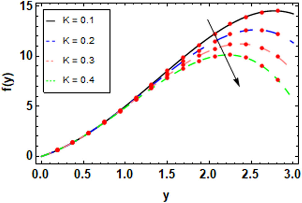
Figures 15 and 16 display the impact of modifying the homogeneous reaction constraint ( K ) and the heterogeneous reaction constraint ( k s ) on the concentration profile. These graphs determine that as the values of K and k s upsurge, the concentration profile diminishes. These actions can be elucidated by the fact that higher reaction rates lead to increased species concentrations, while diffusion rates decrease.

Figure 15

Influence of K on f ( y ) .

$Figure 16 Influence of k s {k}_{{\rm{s}}} on f ( y ) f(y) .$

Figure 16

Influence of k s on f ( y ) .

In Figure 17, the relationship between the Schmidt number ( Sc ) and the concentration profile is depicted. It can be observed that as Sc r rises, the concentration profile improves. Sc is a dimensionless quantity that signifies the ratio of momentum diffusivity to mass diffusivity. Therefore, an intensification in Sc corresponds to an enhancement in the concentration profile.

$Figure 17 Influence of Sc {\rm{Sc}} on f ( y ) f(y) .$

Figure 17

Influence of Sc on f ( y ) .

The influence of the magnetic factor on entropy formation and the Bejan number is depicted in Figure 18(a) and (b). As Mn increases, entropy creation rises while the Bejan number decreases. The occurrence of magnetic fields leads to higher entropy generation in the fluid. With an intensification in the magnetic number, the fluid temperature rises, resulting in enhanced entropy production.

$Figure 18 (a) Influence of Mn {\rm{Mn}} on NG ( y ) {\rm{NG}}(y) . (b) Influence of Mn {\rm{Mn}} on Be {\rm{Be}} .$

Figure 18

(a) Influence of Mn on NG ( y ) . (b) Influence of Mn on Be .

Figure 19(a) and (b) illustrate the stimulus of the Brinkman number Br on entropy creation and the Bejan number. Br represents the relative substance of heat produced by viscous heating compared to heat transferred through molecular conduction. As Br increases, the entropy creation number appears to increase, while the Bejan number diminutions.

$Figure 19 (a) Influence of N N on NG ( y ) {\rm{NG}}(y) . (b) Influence of N N on Be {\rm{Be}} .$

Figure 19

(a) Influence of N on NG ( y ) . (b) Influence of N on Be .

The consequence of the temperature ratio constraint on entropy creation and the Bejan number is presented in Figure 20(a) and (b). As the temperature ratio parameter upsurges, the entropy creation diminutions, while the Bejan number increases in tandem with the temperature ratio parameter.

$Figure 20 (a) Influence of T r {T}_{{\rm{r}}} on NG ( y ) {\rm{NG}}(y) . (b) Influence of T r {T}_{{\rm{r}}} on Be {\rm{Be}} .$

Figure 20

(a) Influence of T r on NG ( y ) . (b) Influence of T r on Be .

The properties of the Reynolds number, Grashof number, and magnetic parameter on the mean pressure drop are shown in Figures 21–23. These figures indicate that the mean pressure drop rises when the magnetic parameter and Reynolds number grow up, while for a higher value of the Grashof number, the mean pressure drop falls. According to these data, the mean pressure drop upsurges with growing magnetic parameters and Reynolds number while decreasing with increasing Grashof numbers. Figure 24(a)–(d) represents the streamlines of the magnetic field, fluid parameter, ratio of diffusion coefficient, and strength of a homogeneous chemical reaction. The figures show that the streamlines increase for accumulative values of the magnetic field, fluid parameter, ratio of diffusion coefficient, and strength of homogeneous chemical reaction.

$Figure 21 Influence of Mn {\rm{Mn}} on ∆ p \triangle p .$

Figure 21

Influence of Mn on ∆ p .

$Figure 22 Influence of Gr {\rm{Gr}} on ∆ p \triangle p .$

Figure 22

Influence of Gr on ∆ p .

$Figure 23 Influence of Re {\rm{Re}} on ∆ p \triangle p .$

Figure 23

Influence of Re on ∆ p .

$Figure 24 Streamlines of (a) magnetic field Mn {\rm{Mn}} , (b) fluid parameter α 1 {\alpha }_{1} , (c) ratio of diffusion coefficient γ \gamma , and (d) strength of homogeneous chemical reaction K K .$

Figure 24

Streamlines of (a) magnetic field Mn , (b) fluid parameter α 1 , (c) ratio of diffusion coefficient γ , and (d) strength of homogeneous chemical reaction K .

Table 1 illustrates the variations in skin friction for different magnetic parameters, velocity slip parameters, Reynolds numbers, and Grashof numbers. It indicates that as the velocity slip parameter and Reynolds number rise, the skin friction coefficient decreases. Conversely, the skin friction coefficient rises as the magnetic factor and Grashof number values rise.

Table 1

The variations in skin friction for a range of different parameters

Mn	α 1	Re	Gr	C f
0.1				2.42806
0.3				2.51904
0.3				2.69993
	0.1			2.42806
	0.3			2.42733
	0.5			2.42659
		0.1		3.011
		0.3		2.42806
		0.5		2.31147
			0.1	2.42806
			0.3	3.011
			0.3	3.59393

Table 2 showcases the changes in the Nusselt number consistent with different magnetic parameters, Eckert numbers, and Grashof numbers. It reveals that the Nusselt number tends to increase for higher values of Eckert and Grashof numbers, as well as for larger magnetic parameter values.

Table 2

Variance of Nusselt number for multiple values of different parameters

Mn	Ec	Gr	N u
0.1			‒ 0.00339919
0.3			‒ 0.0154223
0.5			‒ 0.0394686
	0.1		‒ 0.00306678
	0.3		‒ 0.00378237
	0.5		‒ 0.00449795
		0.1	‒ 0.00339919
		0.3	‒ 0.00577317
		0.3	‒ 0.00909675

7 Conclusions

In this study, we have examined the homogeneous–heterogeneous reaction of MHD peristaltic Oldroyd B fluid flow in a non-uniform vertical channel, considering sliding effects. Our research has explored the potential application of a semi-analytical technique called HAM for solving the nonlinear coupled system with sliding situations. However, instead of using HAM, we have employed graphical representations to illustrate the influence of significant parameters on physiological quantities based on measurable criteria. The main conclusions of this study are as follows:

The velocity declines with cumulative values of the magnetic parameter, retardation parameter, velocity and thermal slip parameters, and Reynolds number. Conversely, the relaxation parameter and Grashof number exhibit an opposite behavior, leading to an upsurge in velocity.
The temperature rises for advanced values of the Eckert number, Grashof number, and magnetic parameter. However, the temperature declines with the cumulative values of the velocity and thermal slip parameters and Reynolds number.
Higher values of the K and k s lead to a degradation of the concentration profile. Conversely, the concentration profile improves for larger values of the Schmidt number.
As the Brinkman number and magnetic parameter increase, the entropy creation number tends to increase, while the Bejan number declines. Alternatively, when the temperature ratio parameter increases, the entropy creation declines and the Bejan number rises.
The mean pressure drop upsurges with advanced values of the magnetic parameter and Reynolds number. However, for a larger value of the Grashof number, the mean pressure drop decreases.
The skin friction coefficient rises for cumulative values of the magnetic parameter and Grashof number. In contrast, it declines with growing values of the velocity slip parameter and Reynolds number.
The Nusselt number increases for larger values of the Eckert number, Grashof number, and magnetic parameter.

Funding information: The project was financed by the Lucian Blaga University of Sibiu through research grant LBUS-IRG-2022-08.
Author contributions: All authors have accepted responsibility for the entire content of this manuscript and approved its submission.
Conflict of interest: The authors state no conflict of interest.

References

[1] Latham TW. Fluid motions in a peristaltic pump. 1966. Accessed: Aug. 14, 2022. [Online]. https://dspace.mit.edu/handle/1721.1/17282.Search in Google Scholar

[2] Fung YC, Yih CS. Peristaltic transport. J Appl Mech. Dec. 1968;35(4):669–75. 10.1115/1.3601290.Search in Google Scholar

[3] Shapiro AH, Jaffrin MY, Weinberg SL. Peristaltic pumping with long wavelengths at low Reynolds number. J Fluid Mech. Jul. 1969;37(4):799–825. 10.1017/S0022112069000899.Search in Google Scholar

[4] Gudekote M, Choudhari R, Vaidya H, Prasad KV, Viharika JU. Influence of convective conditions on the peristaltic mechanism of power-law fluid through a slippery elastic porous tube with different waveforms. Multidiscip Model Mater Struct. Feb. 2020;16(2):340–58. 10.1108/MMMS-01-2019-0006/FULL/XML.Search in Google Scholar

[5] Tanveer A, Khan M, Salahuddin T, Malik MY. Numerical simulation of electroosmosis regulated peristaltic transport of Bingham nanofluid. Comput Methods Prog Biomed. Oct. 2019;180:105005. 10.1016/J.CMPB.2019.105005.Search in Google Scholar PubMed

[6] Rao AR, Usha S. Peristaltic transport of two immiscible viscous fluids in a circular tube. J Fluid Mech. 1995;298:271–85. 10.1017/S0022112095003302.Search in Google Scholar

[7] Raju KK, Devanathan R. Peristaltic motion of a non-Newtonian fluid. Rheol Acta. Jun. 1972;11(2):170–8. 10.1007/BF01993016.Search in Google Scholar

[8] Fetecau C, Prasad SC, Rajagopal KR. A note on the flow induced by a constantly accelerating plate in an Oldroyd-B fluid. Appl Math Model. Apr. 2007;31(4):647–54. 10.1016/J.APM.2005.11.032.Search in Google Scholar

[9] Tiwana MH, Mann AB, Rizwan M, Maqbool K, Javeed S, Raza S, et al. Unsteady magnetohydrodynamic convective fluid flow of Oldroyd-B model considering ramped wall temperature and ramped wall velocity. Mathematics. Jul. 2019;7(8):676. 10.3390/MATH7080676.Search in Google Scholar

[10] Riaz MB, Awrejcewicz J, Rehman AU. Functional effects of permeability on Oldroyd-B fluid under magnetization: A comparison of slipping and non-slipping solutions. Appl Sci. Dec. 2021;11(23):11477. 10.3390/APP112311477.Search in Google Scholar

[11] Boyko E, Stone HA. Pressure-driven flow of the viscoelastic Oldroyd-B fluid in narrow non-uniform geometries: analytical results and comparison with simulations. J Fluid Mech. Apr. 2022;936:A23. 10.1017/JFM.2022.67.Search in Google Scholar

[12] Ibrahim W, Sisay G, Gamachu D. Mixed convection flow of Oldroyd-B nano fluid with Cattaneo-Christov heat and mass flux model with third order slip. AIP Adv. Dec. 2019;9(12):125023. 10.1063/1.5126301.Search in Google Scholar

[13] Ramesh K. Effects of slip and convective conditions on the peristaltic flow of couple stress fluid in an asymmetric channel through porous medium. Comput Methods Prog Biomed. Oct. 2016;135:1–14. 10.1016/J.CMPB.2016.07.001.Search in Google Scholar

[14] Zhang L, Bhatti MM, Michaelides EE. Thermally developed coupled stress particle–fluid motion with mass transfer and peristalsis. J Therm Anal Calorim. Feb. 2021;143(3):2515–24. 10.1007/S10973-020-09871-W.Search in Google Scholar

[15] Abd-Alla AM, Abo-Dahab SM, Thabet EN, Abdelhafez MA. Impact of inclined magnetic field on peristaltic flow of blood fluid in an inclined asymmetric channel in the presence of heat and mass transfer. Waves Random Complex Media. 2022. 10.1080/17455030.2022.2084653.Search in Google Scholar

[16] Nadeem S, Akbar NS, Bibi N, Ashiq S. Influence of heat and mass transfer on peristaltic flow of a third order fluid in a diverging tube. Commun Nonlinear Sci Numer Simul. Oct. 2010;15(10):2916–31. 10.1016/J.CNSNS.2009.11.009.Search in Google Scholar

[17] Ogulu A. Effect of heat generation on low Reynolds number fluid and mass transport in a single lymphatic blood vessel with uniform magnetic field. Int Commun Heat Mass Transf. Jul. 2006;33(6):790–9. 10.1016/J.ICHEATMASSTRANSFER.2006.02.002.Search in Google Scholar

[18] Shafiq A, Lone SA, Sindhu TN, Al-Mdallal QM, Rasool G. Statistical modeling for bioconvective tangent hyperbolic nanofluid towards stretching surface with zero mass flux condition. Sci Rep . Jul. 2021;11(1):1–11. 10.1038/s41598-021-93329-y.Search in Google Scholar PubMed PubMed Central

[19] Wakif A, Animasaun IL, Sehaqui R. A brief technical note on the onset of convection in a horizontal nanofluid layer of finite depth via Wakif-Galerkin weighted residuals technique (WGWRT). Defect Diffus Forum. 2021;409:90–4. 10.4028/WWW.SCIENTIFIC.NET/DDF.409.90.Search in Google Scholar

[20] Iqbal MS, Ghaffari A, Riaz A, Mustafa I, Raza M. Nanofluid transport through a complex wavy geometry with magnetic and permeability effects. Invent. 2022;7(1):7. 10.3390/INVENTIONS7010007. Dec. 2021.Search in Google Scholar

[21] Iqbal MS, Mustafa I, Ghaffari A, Usman. A computational analysis of dissipation effects on the hydromagnetic convective flow of hybrid nanofluids along a vertical wavy surface. Heat Transf. Dec. 2021;50(8):8035–51. 10.1002/HTJ.22265.Search in Google Scholar

[22] Yasmeen S, Okechi NF, Anjum HJ, Asghar S. Peristaltic motion of magnetohydrodynamic viscous fluid in a curved circular tube. Results Phys. Jan. 2017;7:3307–14. 10.1016/J.RINP.2017.08.044.Search in Google Scholar

[23] Srinivas S, Kothandapani M. The influence of heat and mass transfer on MHD peristaltic flow through a porous space with compliant walls. Appl Math Comput. Jul. 2009;213(1):197–208. 10.1016/J.AMC.2009.02.054.Search in Google Scholar

[24] Reddy MG. Heat and mass transfer on magnetohydrodynamic peristaltic flow in a porous medium with partial slip. Alexandria Eng J. 2016;55(2):1225–34. doi: 10.1016/J.AEJ.2016.04.009.Search in Google Scholar

[25] Shahzad H, Ain QU, Pasha AA, Irshad K, Shah IA, Ghaffari A, et al. Double-diffusive natural convection energy transfer in magnetically influenced Casson fluid flow in trapezoidal enclosure with fillets. Int Commun Heat Mass Transf. Oct. 2022;137:106236. 10.1016/J.ICHEATMASSTRANSFER.2022.106236.Search in Google Scholar

[26] Hayat T, Shafiq A, Alsaedi A, Awais M. MHD axisymmetric flow of third grade fluid between stretching sheets with heat transfer. Comput Fluids. Nov. 2013;86:103–8. 10.1016/J.COMPFLUID.2013.07.003.Search in Google Scholar

[27] Hayat T, Shafiq A, Alsaedi A. MHD axisymmetric flow of third grade fluid by a stretching cylinder. Alex Eng J. Jun. 2015;54(2):205–12. 10.1016/J.AEJ.2015.03.013.Search in Google Scholar

[28] Hayat T, Shafiq A, Alsaedi A, Asghar S. Effect of inclined magnetic field in flow of third grade fluid with variable thermal conductivity. AIP Adv. Aug. 2015;5(8):087108. 10.1063/1.4928321.Search in Google Scholar

[29] Rasool G, Wakif A. Numerical spectral examination of EMHD mixed convective flow of second-grade nanofluid towards a vertical Riga plate using an advanced version of the revised Buongiorno’s nanofluid model. J Therm Anal Calorim. Feb. 2021;143(3):2379–93. 10.1007/S10973-020-09865-8/METRICS.Search in Google Scholar

[30] Wakif A, Shah NA. Hydrothermal and mass impacts of azimuthal and transverse components of Lorentz forces on reacting Von Kármán nanofluid flows considering zero mass flux and convective heating conditions. Waves Random Complex Media. 2022. 10.1080/17455030.2022.2136413.Search in Google Scholar

[31] Wakif A, Chamkha A, Thumma T, Animasaun IL, Sehaqui R. Thermal radiation and surface roughness effects on the thermo-magneto-hydrodynamic stability of alumina–copper oxide hybrid nanofluids utilizing the generalized Buongiorno’s nanofluid model. J Therm Anal Calorim. Mar. 2020;143(2):1201–20. 10.1007/S10973-020-09488-Z.Search in Google Scholar

[32] Kothandapani M, Prakash J. Effects of thermal radiation parameter and magnetic field on the peristaltic motion of Williamson nanofluids in a tapered asymmetric channel. Int J Heat Mass Transf. Feb. 2015;81:234–45. 10.1016/J.IJHEATMASSTRANSFER.2014.09.062.Search in Google Scholar

[33] Mebarek-Oudina F. Convective heat transfer of Titania nanofluids of different base fluids in cylindrical annulus with discrete heat source. Heat Transf Res. Jan. 2019;48(1):135–47. 10.1002/HTJ.21375.Search in Google Scholar

[34] Farooq S, Ijaz Khan M, Waqas M, Hayat T, Alsaedi A. Transport of hybrid type nanomaterials in peristaltic activity of viscous fluid considering nonlinear radiation, entropy optimization and slip effects. Comput Methods Prog Biomed. Feb. 2020;184:105086. 10.1016/J.CMPB.2019.105086.Search in Google Scholar

[35] Hayat T, Noreen S, Alsaedi A. Effect of an induced magnetic field on peristaltic flow of non-Newtonian fluid in a curved channel. J Mech Med Biol. Oct. 2012;12(3):1250058. 10.1142/S0219519411004721.Search in Google Scholar

[36] Hayat T, Imtiaz M, Alsaedi A. Impact of magnetohydrodynamics in bidirectional flow of nanofluid subject to second order slip velocity and homogeneous–heterogeneous reactions. J Magn Magn Mater. Dec. 2015;395:294–302. 10.1016/J.JMMM.2015.07.092.Search in Google Scholar

[37] Malik MY, Salahuddin T, Hussain A, Bilal S, Awais M. Homogeneous-heterogeneous reactions in Williamson fluid model over a stretching cylinder by using Keller box method. AIP Adv. Oct. 2015;5(10):107227. 10.1063/1.4934937.Search in Google Scholar

[38] Tanveer A, Hayat T, Alsaedi A, Ahmad B. Mixed convective peristaltic flow of Sisko fluid in curved channel with homogeneous-heterogeneous reaction effects. J Mol Liq. May 2017;233:131–8. 10.1016/J.MOLLIQ.2017.03.001.Search in Google Scholar

[39] Bejan A. Entropy generation minimization: The new thermodynamics of finite-size devices and finite-time processes. J Appl Phys. Feb. 1996;79(3):1191–1218. 10.1063/1.362674.Search in Google Scholar

[40] Khan WA, Ali M. Recent developments in modeling and simulation of entropy generation for dissipative cross material with quartic autocatalysis. Appl Phys A. Jun. 2019;125(6). 10.1007/S00339-019-2686-6.Search in Google Scholar

[41] Rashidi MM, Bhatti MM, Abbas MA, Ali MES. Entropy generation on MHD blood flow of nanofluid due to peristaltic waves. Entropy. Apr. 2016;18(4):117. 10.3390/E18040117.Search in Google Scholar

Received: 2022-12-16

Revised: 2023-03-02

Accepted: 2023-03-16

Published Online: 2023-07-19

This work is licensed under the Creative Commons Attribution 4.0 International License.

Articles in the same Issue

https://doi.org/10.1515/phys-2022-0241

Keywords for this article

Oldroyd-B fluid; MHD; MRI; homogeneous chemical reaction; heterogeneous chemical reaction; entropy generation; Bejan number; HAM

Creative Commons

BY 4.0