Optimal auxiliary function method for analyzing nonlinear system of coupled Schrödinger–KdV equation with Caputo operator
-
 ,
,

Abstract
The optimal auxiliary function method (OAFM) is introduced and used in the analysis of a nonlinear system containing coupled Schrödinger–KdV equations, all within the framework of the Caputo operator. The OAFM, known for its efficiency in solving nonlinear issues, is used to obtain approximate solutions for the coupled equations’ complicated dynamics. Numerical and graphical assessments prove the suggested method’s correctness and efficiency. This study contributes to the understanding and analysis of coupled Schrödinger–KdV equations and their many applications by providing insights into the behavior of nonlinear systems within mathematical physics.
1 Introduction
Fractional partial differential equations (FPDEs) have arisen as a strong mathematical framework for explaining complex systems that show anomalous diffusion, memory effects, and nonlocal interactions. These equations incorporate fractional-order derivatives derived within the context of fractional calculus and so generalize traditional partial differential equations [1–5]. Due to their capacity to simulate complex dynamics that conventional integer-order derivatives cannot fully represent, FPDEs are used in many scientific fields, including biology, engineering, and finance [6–8]. It is possible to trace the theoretical roots of fractional calculus to the pioneering work of mathematicians like Riemann, Liouville, and Caputo [9–11]. However, the promise of FPDEs to provide more precise and realistic representations of diverse natural and artificial systems has only recently attracted substantial attention [12–14]. This introduction’s goal is to give a general understanding of fractional calculus’s core ideas and how they apply to FPDEs while also identifying important sources that have shaped this field’s development [14–18].
The study of nonlinear systems has revealed complex dynamics crucial to several scientific fields. A notable area of study among them is the coupling of the Schrödinger and Korteweg–de Vries (KdV) equations. These equations are important tools for understanding a wide range of physical events because they capture key aspects of wave propagation and soliton processes. The combination of the nonlinear dispersive KdV equation with the quantum mechanical Schrödinger equation results in a coupled system that exhibits intricate interactions between linear and nonlinear processes [19–21]. In addition to offering a more comprehensive framework for comprehending wave dynamics, this coupling also creates opportunities for investigating fascinating phenomena that result from their interdependence. To acquire an understanding of the interaction between quantum and nonlinear dynamics and its larger ramifications across scientific fields, this work investigates the analysis of the nonlinear system of coupled Schrödinger–KdV equations in all of its complexity [22–24].
Understanding the complex behavior of many physical events requires understanding nonlinear systems, which offers an enthralling panorama. The investigation of coupled Schrödinger–KdV equations is one especially fascinating direction in this area. The Schrödinger equation, which regulates the behavior of wave functions in quantum mechanics, and the Korteweg–de Vries equation, which is well known for its role in explaining nonlinear wave propagation and soliton production, are combined in these equations. A new system that captures both linear quantum effects and nonlinear dispersive dynamics is created by linking these equations, offering a singular opportunity to investigate the interactions between these several physical phenomena [25].
In addition to enhancing our knowledge of wave processes, this coupling also has potential applications in several other disciplines, including fluid dynamics and nonlinear optics [26–28]. Understanding the deep links between quantum effects and nonlinear interactions would help researchers understand the complex mechanisms that influence wave behavior in challenging physical contexts [29–31]. This work attempts to reveal the basic insights that result from the coupling of the nonlinear system of coupled Schrödinger–KdV equations, providing a greater understanding of the complicated dynamics and interdependencies that underpin complex wave propagation situations [32,33]. We want to contribute to the better knowledge of nonlinear systems and their importance in various scientific areas via thorough analysis and numerical research [34–36].
The search for efficient methods for resolving nonlinear equations and systems has taken center stage in many scientific fields. The optimal auxiliary function method (OAFM) has emerged as a potential strategy to solve these issues by providing a structured and adaptable framework. The OAFM, which has its roots in mathematical analysis, aims to approximate solutions by carefully including auxiliary functions that improve convergence characteristics. The method’s applicability to various nonlinear situations gives it versatility and makes it useful in disciplines including physics, engineering, and applied mathematics. Using examples from various situations, we examine the theoretical underpinnings, benefits, and practical application of the OAFM in this study [37–39].
Due to its potential for solving challenging nonlinear issues, the OAFM has attracted much interest lately. The OAFM provides a systematic framework for approximation solutions that could otherwise be difficult to acquire by efficiently integrating components of perturbation theory, auxiliary functions, and optimization approaches. The OAFM was used by Lu et al. [40] to tackle nonlinear computational intelligence systems, demonstrating its capacity to extract multiscale characteristics from mixed picture and text input. In the study of Yin et al. [41], a novel end-to-end lake boundary prediction model. This demonstrates how the approach may be used in various fields and highlights its promise as a tool for studying challenging real-world circumstances.
Furthermore, Chen et al. [42], who used the technique to create a generic linear free-energy relationship for forecasting partition coefficients in organic compounds, highlighted the OAFM’s potency in handling mathematical models. This application highlights the OAFM’s ability to draw important correlations from complex mathematical formulations. Furthermore, Lu et al. [43] discussed attention processes in the context of multi-modal fusion in visual question responding, emphasizing how the OAFM might illuminate the intricate interaction of diverse data sources.
The OAFM has shown promise in various applications, from feature extraction to predictive modeling. To contribute to the expanding body of knowledge on efficient nonlinear problem-solving strategies, this work clarifies the method’s theoretical foundations, investigates its benefits, and offers insights into its practical application.
2 Preliminaries
Definition
The fractional Caputo derivative of a function
Definition
The formula for the Riemann fractional integral is as follows:
Lemma
For
3 General procedure of OAFM
To elucidate the fundamental concept of the OAFM, we shall dissect a general nonlinear equation represented as follows:
This equation is accompanied by the given initial/boundary conditions:
In this context,
To initiate this approximation process, we derive the initial and first approximations for Eq. (3) by introducing Eq. (5) into Eq. (3), yielding
The initial approximation, denoted as
The linear operator
To determine the first approximation
accompanied by the following relevant initial/boundary conditions:
Furthermore, the nonlinear term in Eq. (8) can be expanded as follows:
This expansion, as delineated in Eq. (10), can be presented algorithmically to achieve the limiting solution.
In order to overcome the challenges associated with solving the nonlinear differential equation presented in Eq. (6) and expedite the convergence of the first approximation
Remark 1
Remark 2
Remark 3
The nature of
Remark 4
The determination of the values for the unknown parameters
This comprehensive approach underlines the flexibility and adaptability of the OAFM in handling a wide range of nonlinear problems.
3.1 Problem 1
3.1.1 Implementation of OAFM
Consider the coupled Schrödinger–Kdv equation of fractional order
subject to the following initial conditions:
Consider the following linear terms from Eq. (11):
The nonlinear terms can be defined as:
Zeroth order approximation
Using the inverse operator, we obtain the following solution:
Using Eq. (16) in Eq. (14), the system of nonlinear term becomes
and we choose the auxiliary function
The first-order approximation according to OAFM procedure is discussed in Section 3, i.e.,
Using Eqs. (17) and (18) in Eq. (19), we obtain
by applying inverse operator to Eq. (20), we obtain
According to the OAFM procedure,
Using Eqs (16) and (21), we have
The exact result is given as (Tables 1, 2, and 3).
Absolute error of
|
|
Absolute
|
Absolute
|
Absolute
|
|---|---|---|---|
| 0. | 0.00004 | 0.00004 | 0.00004 |
| 0.1 | 0.00130227 | 0.000404499 | 0.000004655 |
| 0.2 | 0.00217469 | 0.000694956 | 0.0000421961 |
| 0.3 | 0.00236032 | 0.000759476 | 0.000053294 |
| 0.4 | 0.00197233 | 0.000635256 | 0.0000454302 |
| 0.5 | 0.0013183 | 0.000423718 | 0.0000290893 |
| 0.6 | 0.000679637 | 0.000217624 | 0.0000138151 |
| 0.7 | 0.000167597 | 0.0000534943 | 0.0000036002 |
| 0.8 | 0.00027163 | 0.0000866903 | 0.00000510754 |
| 0.9 | 0.00074588 | 0.000238765 | 0.00001506 |
| 1. | 0.0012967 | 0.000416593 | 0.0000283522 |
Absolute error of
|
|
Absolute
|
Absolute
|
Absolute
|
|---|---|---|---|
| 0.5 | 0.000577801 | 0.0000354637 | 0.0000281522 |
| 0.6 | 0.00191544 | 0.000181767 | 0.0000215926 |
| 0.7 | 0.0043588 | 0.000452243 | 0.00000599374807 |
| 0.8 | 0.00732438 | 0.000781972 | 0.0000145519 |
| 0.9 | 0.00921167 | 0.000992997 | 0.0000289521 |
| 1. | 0.00812713 | 0.000874782 | 0.0000240854 |
| 1.1 | 0.00317805 | 0.00032797 | 0.0000006343112 |
| 1.2 | 0.0045951 | 0.000532017 | 0.0000554198 |
| 1.3 | 0.0123911 | 0.00139412 | 0.000104191 |
| 1.4 | 0.0169013 | 0.00189093 | 0.000130217 |
| 1.5 | 0.0159235 | 0.00177787 | 0.00011859 |
Absolute error of
|
|
Absolute
|
Absolute
|
Absolute
|
|---|---|---|---|
| 1.3 | 0.000530974 | 0.0000269316 | 0.0000288141 |
| 1.37 | 0.000887848 | 0.0000693315 | 0.0000211942 |
| 1.44 | 0.00131683 | 0.000119502 | 0.0000129191 |
| 1.51 | 0.00178548 | 0.000173845 | 0.00000439 |
| 1.58 | 0.00225593 | 0.000228179 | 0.00000391539 |
| 1.65 | 0.00269217 | 0.000278529 | 0.000011588 |
| 1.72 | 0.00306528 | 0.000321714 | 0.0000182843 |
| 1.79 | 0.00335612 | 0.000355633 | 0.0000237875 |
| 1.86 | 0.00355569 | 0.000379302 | 0.0000280033 |
| 1.93 | 0.00366383 | 0.00039272 | 0.0000309441 |
| 2. | 0.00368713 | 0.000396623 | 0.0000327027 |
4 Numerical and graphical results
The graphical analysis in this section provides insights into the behavior of the solutions to the nonlinear system of coupled Schrodinger–KdV equations with varying fractional orders (
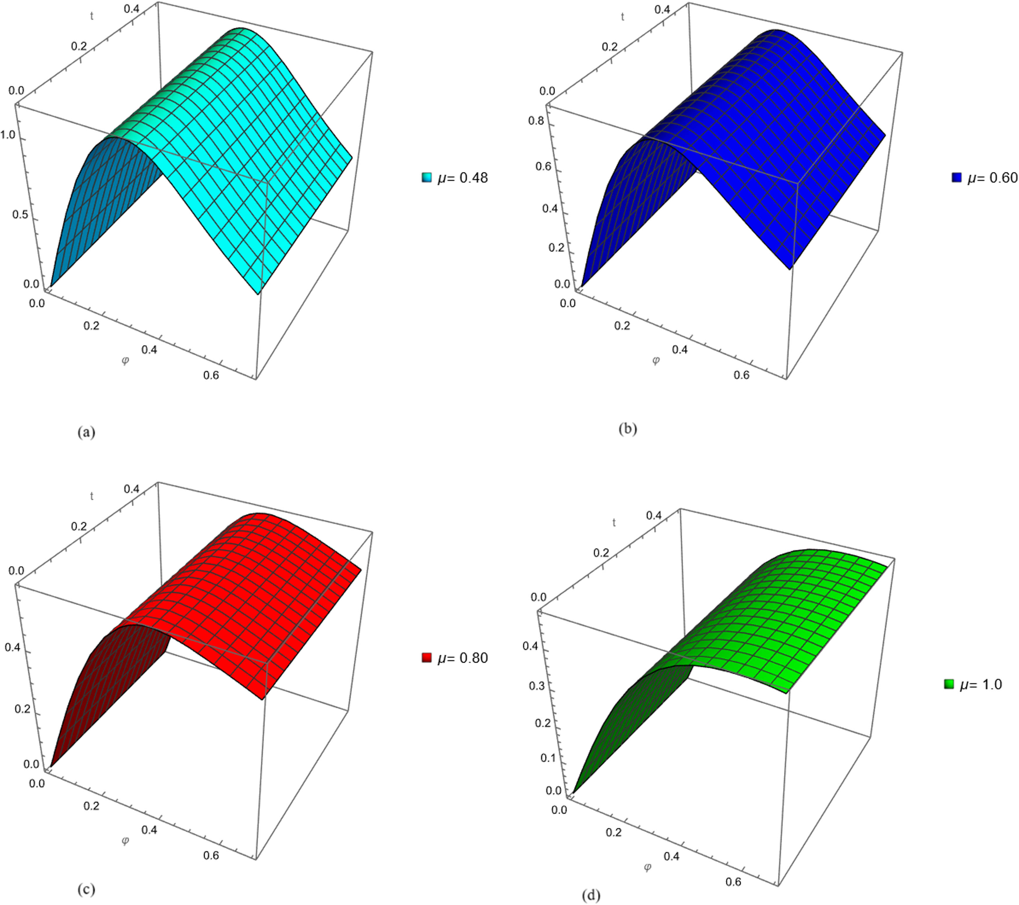
The fractional order of (a)
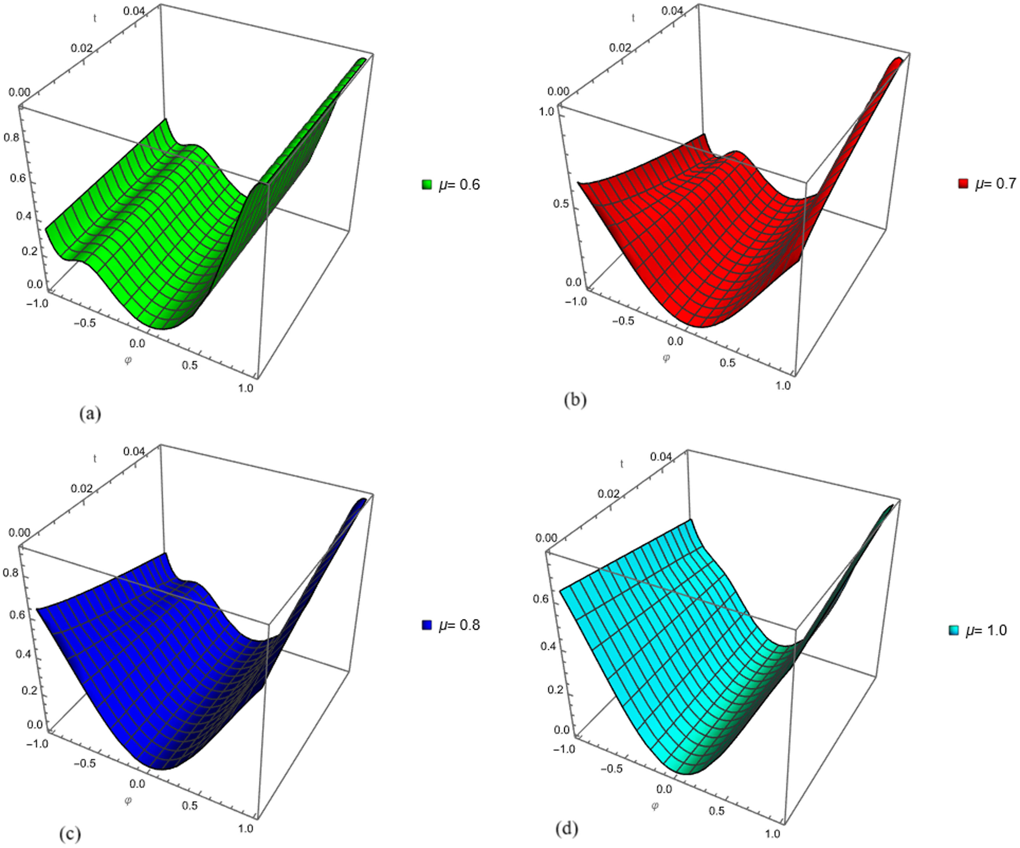
The fractional order of (a)
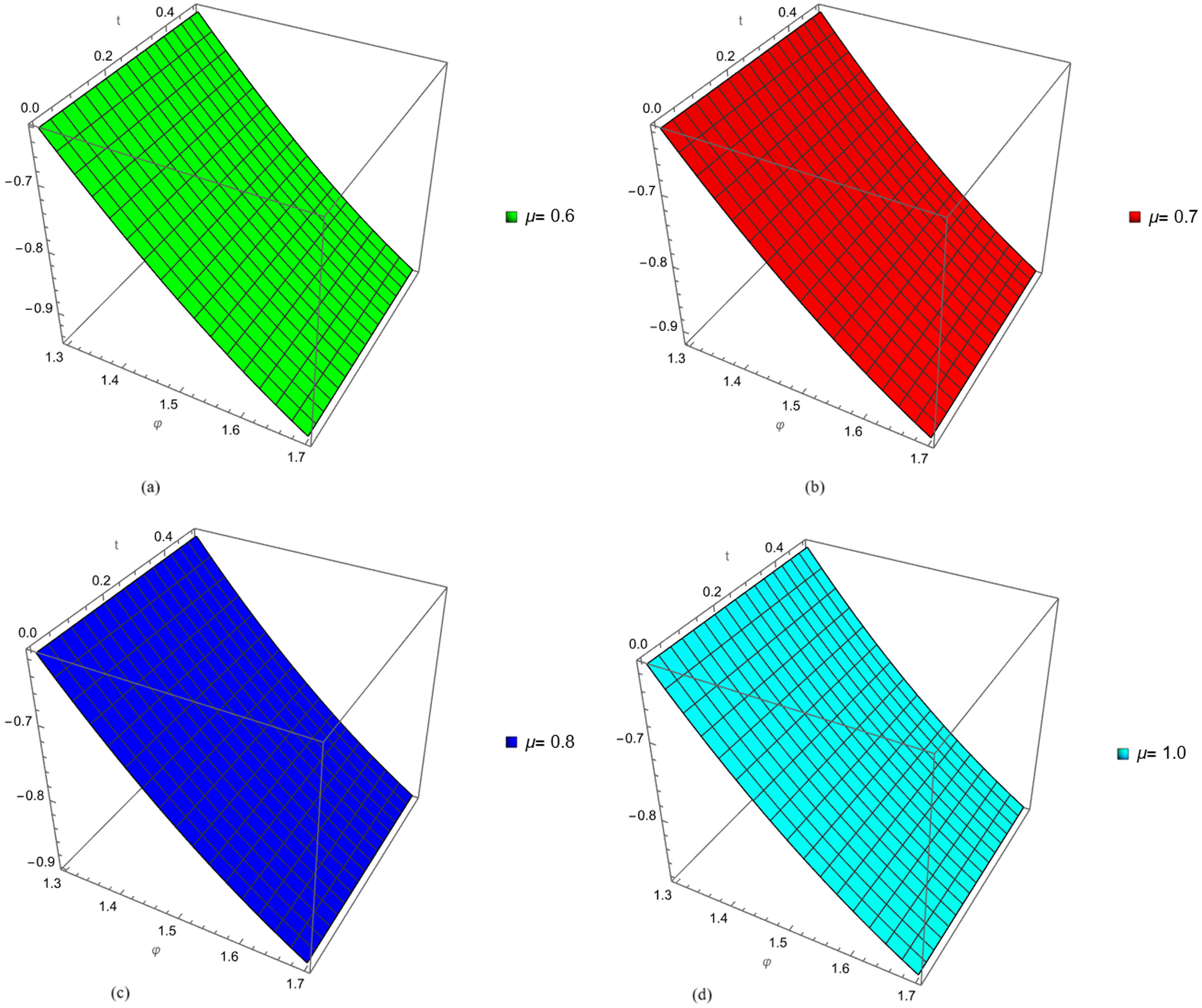
The fractional order of (a)
5 Conclusion
Finally, this research ventured into the domain of nonlinear systems by using the OAFM to evaluate a coupled system of Schrödinger–KdV equations using the Caputo operator. The OAFM demonstrated its effectiveness in handling difficult nonlinear issues by approximating solutions to the intricate dynamics of the coupled equations. The reported numerical and graphical assessments proved the method’s correctness and efficiency, demonstrating its potential for dealing with difficult mathematical physics problems. This research adds to a greater knowledge of coupled Schrödinger–KdV equations and their ramifications across numerous scientific areas by effectively revealing insights into the behavior of the nonlinear system. The OAFM’s relevance as a useful instrument in the arsenal of mathematical analysis is reinforced by its capacity to offer trustworthy solutions to complex nonlinear systems.
Acknowlegments
This work received support from the Princess Nourah bint Abdulrahman University Researchers Supporting Project number (PNURSP2023R183), Princess Nourah bint Abdulrahman University, Riyadh, Saudi Arabia. This work was supported by the Deanship of Scientific Research, the Vice Presidency for Graduate Studies and Scientific Research, King Faisal University, Saudi Arabia (Grant No. 4447).
-
Funding information: This work received support from the Princess Nourah bint Abdulrahman University Researchers Supporting Project number (PNURSP2023R183), Princess Nourah bint Abdulrahman University, Riyadh, Saudi Arabia. This work was supported by the Deanship of Scientific Research, the Vice Presidency for Graduate Studies and Scientific Research, King Faisal University, Saudi Arabia (Grant No. 4447).
-
Author contributions: All authors have accepted responsibility for the entire content of this manuscript and approved its submission.
-
Conflict of interest: The authors state no conflict of interest.
References
[1] Deepika S, Veeresha P. Dynamics of chaotic waterwheel model with the asymmetric flow within the frame of Caputo fractional operator. Chaos Solitons Fractals. 2023;169:113298. 10.1016/j.chaos.2023.113298Search in Google Scholar
[2] Premakumari RN, Baishya C, Veeresha P, Akinyemi L. A fractional atmospheric circulation system under the influence of a sliding mode controller. Symmetry. 2022;14(12):2618. 10.3390/sym14122618Search in Google Scholar
[3] Ilhan E, Veeresha P, Baskonus HM. Fractional approach for a mathematical model of atmospheric dynamics of CO2 gas with an efficient method. Chaos Solitons Fractals. 2021;152:111347. 10.1016/j.chaos.2021.111347Search in Google Scholar
[4] Gao W, Veeresha P, Cattani C, Baishya C, Baskonus HM. Modified predictor-corrector method for the numerical solution of a fractional-order SIR model with 2019-nCoV. Fractal and Fractional, 2022;6(2):92. 10.3390/fractalfract6020092Search in Google Scholar
[5] Akinyemi L, Veeresha P, Ajibola SO. Numerical simulation for coupled nonlinear Schrodinger-Korteweg–de Vries and Maccari systems of equations. Modern Phys Lett B. 2021;35(20):2150339. 10.1142/S0217984921503395Search in Google Scholar
[6] Veeresha P, Ilhan E, Baskonus HM. Fractional approach for analysis of the model describing wind-influenced projectile motion. Physica Scripta. 2021;96(7):075209. 10.1088/1402-4896/abf868Search in Google Scholar
[7] Alderremy AA, Aly S, Fayyaz R, Khan A, Wyal N. The analysis of fractional-order nonlinear systems of third order KdV and Burgers equations via a novel transform. Complexity. 2022;2022:4935809. 10.1155/2022/4935809Search in Google Scholar
[8] Fu H, Wang H, Wang Z. POD/DEIM reduced-order modeling of time-fractional partial differential equations with applications in parameter identification. J Scientif Comput. 2018;74:220–43. 10.1007/s10915-017-0433-8Search in Google Scholar
[9] Sunthrayuth P, Aljahdaly NH, Ali A, Mahariq I, Tchalla AM. psi-Haar wavelet operational matrix method for fractional relaxation-oscillation equations containing ψ-Caputo fractional derivative. J Funct Spaces. 2021;2021:1–14. 10.1155/2021/7117064Search in Google Scholar
[10] Yasmin H, Aljahdaly NH, Saeed AM. Probing families of optical soliton solutions in fractional perturbed Radhakrishnan-Kundu-Lakshmanan model with improved versions of extended direct algebraic method. Fractal Fraction 2023;7(7):512. Search in Google Scholar
[11] Yasmin H, Alshehry AS, Khan A, Nonlaopon K. Numerical analysis of the fractional-order Belousov-Zhabotinsky system. Symmetry. 2023;15(4):834. 10.3390/sym15040834Search in Google Scholar
[12] Veeresha P. The efficient fractional order based approach to analyze chemical reaction associated with pattern formation. Chaos Solitons Fractals. 2022;165:112862. 10.1016/j.chaos.2022.112862Search in Google Scholar
[13] Song J, Mingotti A, Zhang J, Peretto L, Wen H. Accurate damping factor and frequency estimation for damped real-valued sinusoidal signals. IEEE Trans Instrument Measurement. 2022;71:6503504. 10.1109/TIM.2022.3220300. Search in Google Scholar
[14] Hu D, Li Y, Yang X, Liang X, Zhang K, Liang X, et al. Experiment and application of NATM tunnel deformation monitoring based on 3D laser scanning. Struct Control Health Monitor. 2023;2023:3341788. 10.1155/2023/3341788. Search in Google Scholar
[15] Guo C, Hu J, Hao J, Celikovsky S, Hu X. Fixed-time safe tracking control of uncertain high-order nonlinear pure-feedback systems via unified transformation functions. Kybernetika. 2023;59(3):342–64. 10.14736/kyb-2023-3-0342. Search in Google Scholar
[16] Yasmin H, Aljahdaly NH, Saeed AM, Shah R. Probing families of optical soliton solutions in fractional perturbed Radhakrishnan-Kundu-Lakshmanan model with improved versions of extended direct algebraic method. Fractal Fractional. 2023;7(7):512. 10.3390/fractalfract7070512Search in Google Scholar
[17] Yasmin H, Aljahdaly NH, Saeed AM. Investigating families of soliton solutions for the complex structured coupled fractional Biswas-Arshed model in birefringent fibers using a novel analytical technique. Fractal Fractional. 2023;7(7):491. 10.3390/fractalfract7070491Search in Google Scholar
[18] Yasmin H, Aljahdaly NH, Saeed AM, Shah R. Investigating symmetric soliton solutions for the fractional coupled Konno-Onno system using improved versions of a novel analytical technique. Mathematics. 2023;11(12):2686. 10.3390/math11122686Search in Google Scholar
[19] Shafee A, Alkhezi Y. Efficient solution of fractional system partial differential equations using Laplace residual power series method. Fractal Fract. 2023;7(6):429. 10.3390/fractalfract7060429Search in Google Scholar
[20] Mason LJ, Sparling GA. Nonlinear Schrödinger and Korteweg–de Vries are reductions of self-dual Yang-Mills. Phys Lett A. 1989;137(1–2):29–33. 10.1016/0375-9601(89)90964-XSearch in Google Scholar
[21] Klein C. Fourth order time-stepping for low dispersion Korteweg–de Vries and nonlinear Schrödinger equation. Electron Trans Numer Anal. 2008;29(116–135):37. Search in Google Scholar
[22] Noor S, Alotaibi BM, Ismaeel SM, El-Tantawy SA. On the solitary waves and nonlinear oscillations to the fractional Schrödinger-KdV equation in the framework of the Caputo operator. Symmetry. 2023;15(8):1616. 10.3390/sym15081616Search in Google Scholar
[23] Alshammari S, Al-Sawalha MM. Approximate analytical methods for a fractional-order nonlinear system of Jaulent-Miodek equation with energy-dependent Schrödinger potential. Fractal Fract. 2023;7(2):140. 10.3390/fractalfract7020140Search in Google Scholar
[24] Shah R, Hyder AA, Iqbal N, Botmart T Fractional view evaluation system of Schrödinger-KdV equation by a comparative analysis. AIMS Math. 2022;7(11):19846–64. 10.3934/math.20221087Search in Google Scholar
[25] Bekiranov D, Ogawa T, Ponce G. Weak solvability and well-posedness of a coupled Schrodinger-Korteweg de Vries equation for capillary-gravity wave interactions. Proc Amer Math Soc. 1997;125(10):2907–19. 10.1090/S0002-9939-97-03941-5Search in Google Scholar
[26] Guo C, Hu J, Wu Y, Celikovsky S. Non-singular fixed-time tracking control of uncertain nonlinear pure-feedback systems with practical state constraints. IEEE Trans Circuits Syst I Regular Papers. 2023;70(9):3746–58. 10.1109/TCSI.2023.3291700. Search in Google Scholar
[27] Meng Q, Ma Q, Shi Y. Adaptive fixed-time stabilization for a class of uncertain nonlinear systems. IEEE Trans Automatic Control. 2023. 10.1109/TAC.2023.3244151. Search in Google Scholar
[28] Ma Q, Meng Q, Xu S. Distributed optimization for uncertain high-order nonlinear multiagent systems via dynamic gain approach. IEEE Trans Syst Man Cybernetics Syst. 2023;53(7):4351–7. 10.1109/TSMC.2023.3247456. Search in Google Scholar
[29] Colorado E. On the existence of bound and ground states for some coupled nonlinear Schrodinger-Korteweg–de Vries equations. Adv Nonlinear Anal. 2017;6(4):407–26. 10.1515/anona-2015-0181Search in Google Scholar
[30] Song M, Qian X, Zhang H, Song S. Hamiltonian boundary value method for the nonlinear Schrodinger equation and the Korteweg–de Vries equation. Adv Appl Math Mechanics. 2017;9(4):868–86. 10.4208/aamm.2015.m1356Search in Google Scholar
[31] Liu Q, Peng H, Wang Z. Convergence to nonlinear diffusion waves for a hyperbolic-parabolic chemotaxis system modelling vasculogenesis. J Differ Equ. 2022;314:251–86. https://doi.org/10.1016/j.jde.2022.01.021. Search in Google Scholar
[32] Jin H, Wang Z, Wu L. Global dynamics of a three-species spatial food chain model. J Differ Equ. 2022;333:144–83. https://doi.org/10.1016/j.jde.2022.06.007. Search in Google Scholar
[33] Wang B, Shen Y, Li N, Zhang Y, Gao Z. An adaptive sliding mode fault-tolerant control of a quadrotor unmanned aerial vehicle with actuator faults and model uncertainties. Int J Robust Nonlinear Control. 2023. https://doi.org/10.1002/rnc.6631. 10.1002/rnc.6631Search in Google Scholar
[34] Wang B, Zhang Y, Zhang W. A composite adaptive fault-tolerant attitude control for a quadrotor UAV with multiple uncertainties. J Syst Sci Complexity. 2022;35(1):81–104. 10.1007/s11424-022-1030-y. Search in Google Scholar
[35] Li Q, Lin H, Tan X, Du S. H-∞ consensus for multiagent-based supply chain systems under switching topology and uncertain demands. IEEE Trans Syst Man Cybernetics Syst. 2020;50(12):4905–18. https://doi.org/10.1109/TSMC.2018.2884510. Search in Google Scholar
[36] Zhang X, Lu Z, Yuan X, Wang Y, Shen X. L2-gain adaptive robust control for hybrid energy storage system in electric vehicles. IEEE Trans Power Electron. 2021;36(6):7319–32. https://doi.org/10.1109/TPEL.2020.3041653. Search in Google Scholar
[37] Taghieh A, Zhang C, Alattas KA, Bouteraa Y, Rathinasamy S, Mohammadzadeh A. A predictive type-3 fuzzy control for underactuated surface vehicles. Ocean Eng. 2022;266:113014. https://doi.org/10.1016/j.oceaneng.2022.113014. Search in Google Scholar
[38] Bai X, He Y, Xu M. Low-thrust reconfiguration strategy and optimization for formation flying using Jordan normal form. IEEE Trans Aerospace Electronic Syst. 2021;57(5):3279–95. https://doi.org/10.1109/TAES.2021.3074204. Search in Google Scholar
[39] Sun W, Wang H, Qu R. A novel data generation and quantitative characterization method of motor static eccentricity with adversarial network. IEEE Trans Power Electronics. 2023;38(7):8027–32. https://doi.org/10.1109/TPEL.2023.3267883. Search in Google Scholar
[40] Lu S, Ding Y, Liu M, Yin Z, Yin L, Zheng W. Multiscale feature extraction and fusion of image and text in VQA. Int J Comput Intell Syst. 2020;16(1):54. https://doi.org/10.1007/s44196-023-00233-6. Search in Google Scholar
[41] Yin L, Wang L, Li T, Lu S, Yin Z, Liu X, et al. U-Net-STN: A novel end-to-end lake boundary prediction model. Land. 2023;12(8):1602. 10.3390/land12081602. Search in Google Scholar
[42] Chen D, Wang Q, Li Y, Li Y, Zhou H, Fan Y. A general linear free energy relationship for predicting partition coefficients of neutral organic compounds. Chemosphere. 2020;247:125869. 10.1016/j.chemosphere.2020.125869. Search in Google Scholar PubMed
[43] Lu S, Liu M, Yin L, Yin Z, Liu X, Zheng W, et al. The multi-modal fusion in visual question answering: a review of attention mechanisms. Peer J Comput Sci. 2023;9:e1400. 10.7717/peerj-cs.1400. Search in Google Scholar PubMed PubMed Central
© 2023 the author(s), published by De Gruyter
This work is licensed under the Creative Commons Attribution 4.0 International License.
Articles in the same Issue
- Regular Articles
- Dynamic properties of the attachment oscillator arising in the nanophysics
- Parametric simulation of stagnation point flow of motile microorganism hybrid nanofluid across a circular cylinder with sinusoidal radius
- Fractal-fractional advection–diffusion–reaction equations by Ritz approximation approach
- Behaviour and onset of low-dimensional chaos with a periodically varying loss in single-mode homogeneously broadened laser
- Ammonia gas-sensing behavior of uniform nanostructured PPy film prepared by simple-straightforward in situ chemical vapor oxidation
- Analysis of the working mechanism and detection sensitivity of a flash detector
- Flat and bent branes with inner structure in two-field mimetic gravity
- Heat transfer analysis of the MHD stagnation-point flow of third-grade fluid over a porous sheet with thermal radiation effect: An algorithmic approach
- Weighted survival functional entropy and its properties
- Bioconvection effect in the Carreau nanofluid with Cattaneo–Christov heat flux using stagnation point flow in the entropy generation: Micromachines level study
- Study on the impulse mechanism of optical films formed by laser plasma shock waves
- Analysis of sweeping jet and film composite cooling using the decoupled model
- Research on the influence of trapezoidal magnetization of bonded magnetic ring on cogging torque
- Tripartite entanglement and entanglement transfer in a hybrid cavity magnomechanical system
- Compounded Bell-G class of statistical models with applications to COVID-19 and actuarial data
- Degradation of Vibrio cholerae from drinking water by the underwater capillary discharge
- Multiple Lie symmetry solutions for effects of viscous on magnetohydrodynamic flow and heat transfer in non-Newtonian thin film
- Thermal characterization of heat source (sink) on hybridized (Cu–Ag/EG) nanofluid flow via solid stretchable sheet
- Optimizing condition monitoring of ball bearings: An integrated approach using decision tree and extreme learning machine for effective decision-making
- Study on the inter-porosity transfer rate and producing degree of matrix in fractured-porous gas reservoirs
- Interstellar radiation as a Maxwell field: Improved numerical scheme and application to the spectral energy density
- Numerical study of hybridized Williamson nanofluid flow with TC4 and Nichrome over an extending surface
- Controlling the physical field using the shape function technique
- Significance of heat and mass transport in peristaltic flow of Jeffrey material subject to chemical reaction and radiation phenomenon through a tapered channel
- Complex dynamics of a sub-quadratic Lorenz-like system
- Stability control in a helicoidal spin–orbit-coupled open Bose–Bose mixture
- Research on WPD and DBSCAN-L-ISOMAP for circuit fault feature extraction
- Simulation for formation process of atomic orbitals by the finite difference time domain method based on the eight-element Dirac equation
- A modified power-law model: Properties, estimation, and applications
- Bayesian and non-Bayesian estimation of dynamic cumulative residual Tsallis entropy for moment exponential distribution under progressive censored type II
- Computational analysis and biomechanical study of Oldroyd-B fluid with homogeneous and heterogeneous reactions through a vertical non-uniform channel
- Predictability of machine learning framework in cross-section data
- Chaotic characteristics and mixing performance of pseudoplastic fluids in a stirred tank
- Isomorphic shut form valuation for quantum field theory and biological population models
- Vibration sensitivity minimization of an ultra-stable optical reference cavity based on orthogonal experimental design
- Effect of dysprosium on the radiation-shielding features of SiO2–PbO–B2O3 glasses
- Asymptotic formulations of anti-plane problems in pre-stressed compressible elastic laminates
- A study on soliton, lump solutions to a generalized (3+1)-dimensional Hirota--Satsuma--Ito equation
- Tangential electrostatic field at metal surfaces
- Bioconvective gyrotactic microorganisms in third-grade nanofluid flow over a Riga surface with stratification: An approach to entropy minimization
- Infrared spectroscopy for ageing assessment of insulating oils via dielectric loss factor and interfacial tension
- Influence of cationic surfactants on the growth of gypsum crystals
- Study on instability mechanism of KCl/PHPA drilling waste fluid
- Analytical solutions of the extended Kadomtsev–Petviashvili equation in nonlinear media
- A novel compact highly sensitive non-invasive microwave antenna sensor for blood glucose monitoring
- Inspection of Couette and pressure-driven Poiseuille entropy-optimized dissipated flow in a suction/injection horizontal channel: Analytical solutions
- Conserved vectors and solutions of the two-dimensional potential KP equation
- The reciprocal linear effect, a new optical effect of the Sagnac type
- Optimal interatomic potentials using modified method of least squares: Optimal form of interatomic potentials
- The soliton solutions for stochastic Calogero–Bogoyavlenskii Schiff equation in plasma physics/fluid mechanics
- Research on absolute ranging technology of resampling phase comparison method based on FMCW
- Analysis of Cu and Zn contents in aluminum alloys by femtosecond laser-ablation spark-induced breakdown spectroscopy
- Nonsequential double ionization channels control of CO2 molecules with counter-rotating two-color circularly polarized laser field by laser wavelength
- Fractional-order modeling: Analysis of foam drainage and Fisher's equations
- Thermo-solutal Marangoni convective Darcy-Forchheimer bio-hybrid nanofluid flow over a permeable disk with activation energy: Analysis of interfacial nanolayer thickness
- Investigation on topology-optimized compressor piston by metal additive manufacturing technique: Analytical and numeric computational modeling using finite element analysis in ANSYS
- Breast cancer segmentation using a hybrid AttendSeg architecture combined with a gravitational clustering optimization algorithm using mathematical modelling
- On the localized and periodic solutions to the time-fractional Klein-Gordan equations: Optimal additive function method and new iterative method
- 3D thin-film nanofluid flow with heat transfer on an inclined disc by using HWCM
- Numerical study of static pressure on the sonochemistry characteristics of the gas bubble under acoustic excitation
- Optimal auxiliary function method for analyzing nonlinear system of coupled Schrödinger–KdV equation with Caputo operator
- Analysis of magnetized micropolar fluid subjected to generalized heat-mass transfer theories
- Does the Mott problem extend to Geiger counters?
- Stability analysis, phase plane analysis, and isolated soliton solution to the LGH equation in mathematical physics
- Effects of Joule heating and reaction mechanisms on couple stress fluid flow with peristalsis in the presence of a porous material through an inclined channel
- Bayesian and E-Bayesian estimation based on constant-stress partially accelerated life testing for inverted Topp–Leone distribution
- Dynamical and physical characteristics of soliton solutions to the (2+1)-dimensional Konopelchenko–Dubrovsky system
- Study of fractional variable order COVID-19 environmental transformation model
- Sisko nanofluid flow through exponential stretching sheet with swimming of motile gyrotactic microorganisms: An application to nanoengineering
- Influence of the regularization scheme in the QCD phase diagram in the PNJL model
- Fixed-point theory and numerical analysis of an epidemic model with fractional calculus: Exploring dynamical behavior
- Computational analysis of reconstructing current and sag of three-phase overhead line based on the TMR sensor array
- Investigation of tripled sine-Gordon equation: Localized modes in multi-stacked long Josephson junctions
- High-sensitivity on-chip temperature sensor based on cascaded microring resonators
- Pathological study on uncertain numbers and proposed solutions for discrete fuzzy fractional order calculus
- Bifurcation, chaotic behavior, and traveling wave solution of stochastic coupled Konno–Oono equation with multiplicative noise in the Stratonovich sense
- Thermal radiation and heat generation on three-dimensional Casson fluid motion via porous stretching surface with variable thermal conductivity
- Numerical simulation and analysis of Airy's-type equation
- A homotopy perturbation method with Elzaki transformation for solving the fractional Biswas–Milovic model
- Heat transfer performance of magnetohydrodynamic multiphase nanofluid flow of Cu–Al2O3/H2O over a stretching cylinder
- ΛCDM and the principle of equivalence
- Axisymmetric stagnation-point flow of non-Newtonian nanomaterial and heat transport over a lubricated surface: Hybrid homotopy analysis method simulations
- HAM simulation for bioconvective magnetohydrodynamic flow of Walters-B fluid containing nanoparticles and microorganisms past a stretching sheet with velocity slip and convective conditions
- Coupled heat and mass transfer mathematical study for lubricated non-Newtonian nanomaterial conveying oblique stagnation point flow: A comparison of viscous and viscoelastic nanofluid model
- Power Topp–Leone exponential negative family of distributions with numerical illustrations to engineering and biological data
- Extracting solitary solutions of the nonlinear Kaup–Kupershmidt (KK) equation by analytical method
- A case study on the environmental and economic impact of photovoltaic systems in wastewater treatment plants
- Application of IoT network for marine wildlife surveillance
- Non-similar modeling and numerical simulations of microploar hybrid nanofluid adjacent to isothermal sphere
- Joint optimization of two-dimensional warranty period and maintenance strategy considering availability and cost constraints
- Numerical investigation of the flow characteristics involving dissipation and slip effects in a convectively nanofluid within a porous medium
- Spectral uncertainty analysis of grassland and its camouflage materials based on land-based hyperspectral images
- Application of low-altitude wind shear recognition algorithm and laser wind radar in aviation meteorological services
- Investigation of different structures of screw extruders on the flow in direct ink writing SiC slurry based on LBM
- Harmonic current suppression method of virtual DC motor based on fuzzy sliding mode
- Micropolar flow and heat transfer within a permeable channel using the successive linearization method
- Different lump k-soliton solutions to (2+1)-dimensional KdV system using Hirota binary Bell polynomials
- Investigation of nanomaterials in flow of non-Newtonian liquid toward a stretchable surface
- Weak beat frequency extraction method for photon Doppler signal with low signal-to-noise ratio
- Electrokinetic energy conversion of nanofluids in porous microtubes with Green’s function
- Examining the role of activation energy and convective boundary conditions in nanofluid behavior of Couette-Poiseuille flow
- Review Article
- Effects of stretching on phase transformation of PVDF and its copolymers: A review
- Special Issue on Transport phenomena and thermal analysis in micro/nano-scale structure surfaces - Part IV
- Prediction and monitoring model for farmland environmental system using soil sensor and neural network algorithm
- Special Issue on Advanced Topics on the Modelling and Assessment of Complicated Physical Phenomena - Part III
- Some standard and nonstandard finite difference schemes for a reaction–diffusion–chemotaxis model
- Special Issue on Advanced Energy Materials - Part II
- Rapid productivity prediction method for frac hits affected wells based on gas reservoir numerical simulation and probability method
- Special Issue on Novel Numerical and Analytical Techniques for Fractional Nonlinear Schrodinger Type - Part III
- Adomian decomposition method for solution of fourteenth order boundary value problems
- New soliton solutions of modified (3+1)-D Wazwaz–Benjamin–Bona–Mahony and (2+1)-D cubic Klein–Gordon equations using first integral method
- On traveling wave solutions to Manakov model with variable coefficients
- Rational approximation for solving Fredholm integro-differential equations by new algorithm
- Special Issue on Predicting pattern alterations in nature - Part I
- Modeling the monkeypox infection using the Mittag–Leffler kernel
- Spectral analysis of variable-order multi-terms fractional differential equations
- Special Issue on Nanomaterial utilization and structural optimization - Part I
- Heat treatment and tensile test of 3D-printed parts manufactured at different build orientations