Extracting solitary solutions of the nonlinear Kaup–Kupershmidt (KK) equation by analytical method

Mohammed Shaaf Alharthi

doi:10.1515/phys-2023-0134

Artikel Open Access

Extracting solitary solutions of the nonlinear Kaup–Kupershmidt (KK) equation by analytical method

Mohammed Shaaf Alharthi

Veröffentlicht/Copyright: 19. Dezember 2023

Veröffentlicht von

Veröffentlichen auch Sie bei De Gruyter Brill

Manuskript einreichen Informationen für Autor*innen Erkunden Sie dieses Fachgebiet

Aus der Zeitschrift Open Physics Band 21 Heft 1

Abstract

Finding analytical solutions for nonlinear partial differential equations is physically meaningful. The Kaup-Kupershmidt (KK) equation is studied in this article. The KK equation is of fifth order, such that several solitary solutions are obtained. In this article, however, the modified auxiliary function approach is applied to this model to find solitary solutions. These solutions are written in terms of Jacobi functions. Therefore, the obtained solutions can be implemented graphically to show different patterns for appropriate parameters.

Keywords: solitary waves; solitons; exact solutions; Jacobi functions; exponential solution

1 Introduction

Nonlinear partial differential equations (NPDEs) govern transport phenomena that manifest in various physics and engineering scenarios. These partial differential equations can be used to model, for instance, solitary waves in fluid problems such as earthquakes and the hydromagnetic flux of a dusty liquid through a porous medium [1] or fluid dynamics such as Bona–Mahony equation [2–5], Benney-Luke equation, the modified Kortewege–de-Varies equation [6,7], heat transfer in thermoelectric fluid [8] and Benjamin–Bona–Mohaony equation [9,10]. Great attention has already been taken to the Kaup–Kupershmidt (KK) equation [11,12] and also to Sawada–Kotera model [13] that are fifth-order NPDEs.

In literature, the latter two equations are well documented even though they are of the same order and different. The KK model is more complex than the Sawada–Kotera model regarding integrability and mathematical solutions. However, the KK equation is still an active system as far as we know of which one would seek further soliton solutions. The KK equation can be applied to various applications in physics, such as nonlinear optics, fluid dynamics, and plasma physics [14]. In 1980, the famous classical KK equation is introduced by Kaup [15] and modified by Kupershmidt in 1994 [16]. Most recently, numerical approaches to the fractional-order KK equation have been implemented to seek nonlinear dispersive waves and capillary gravity waves [17]. For fractional-order differential equations model, readers who express interest in the topic are advised to consult these references [18–23].

In the literature, Kaup found numerically solitary solutions to the KK equation by using inverse scattering theory. Herman and Nusier [24] have computed two and three solutions, but, they did not provide a further sequence of soliton solutions. This brought motivation to investigate the existence of exact solutions with the aid of Mathematica software and several analytical methods. For instance, the modified auxiliary equation (MAE) method [25,26], the exponential expansion method [27], the tanh-based expansion method [28], the Jacobi elliptic functions method [29], the modified exponential rational method [30], the G ′ ∕ G -expansion method [31] with interested applications, and the Kudryashov method [32]. Moreover, one may refer to [33,34] for more analytical methods, for instance, the sub-equation method and more. Furthermore, several computational methods can be used to approximate soliton solutions, such as the Adomian decomposition approach [35], homotopy analyzis approach [36], and Laplace-homotopy perturbation method [37].

The objective of this present manuscript is to investigate new traveling wave solutions to the problem under investigation. This includes exponential periodic hyperbolic [2–4] and rational [4,5] analytical solutions different from those exposed in the literature. The analytical method MAE is utilized to construct different analytical solutions for the KK equation using the well-known Jacobi functions. Further solitons solution is determined and analyzed upon any constraint conditions if they exist. Furthermore, the solutions are displayed graphically and classified according to the Soliton profiles.

The current manuscript is organized as follows: an overview of the methodology used herein in Section 2; in Section 3, we use the proposed approach to the KK equation; Section 4 is devoted to discussing the obtained solutions; and at the end of Section 5, the conclusion and further ideas are presented.

2 The method of MAE

Here, we give an overview of the modified auxiliary method [25,26]. Thus, consider the general form of the NPDEs as follows:

(1) χ ( υ , υ x , υ t , υ x t , υ x x , … ) = 0 ,

where υ = χ ( x , t ) is unknown function in space and time, respectively.

The outline of the method is presented as follows as:

Step 1: we apply the following transformation:
(2) χ ( x , t ) = W ( ζ ) , ζ = x + c 1 t ,
where c 1 is arbitrary constant. Then, employing the applied transformation in Eq. (2) to the partial equation in Eq. (1), it will be converted to an ordinary differential equation in the following nonlinear form:
(3) Q ( W , W ′ , W ″ , W ‴ , … ) | = 0 .
Step 2: Assuming the solution of Eq. (3) would be
(4) W ( ζ ) = ∑ j = − n n η j Ψ j ( ζ )
such that n > 0 is an integer and η j are constants that will be specified. The function Ψ j ( ζ ) satisfies:
(5) Ψ ′ 2 ( ζ ) = υ 0 + υ 1 Ψ 2 ( ζ ) + υ 2 Ψ 4 ( ζ ) ,
where υ 0 , υ 1 , and υ 2 are arbitrary constants. Therefore, Eq. (5) admits several solutions’ cases as follows:
- Case 1: If υ 0 = 1 , υ 1 = − ( 1 + k 2 ) , and υ 2 = k 2 , then the solution to Eq. (5) is: Ψ ( ζ ) = s n ( ζ , k ) , where s n ( ζ , k ) is the Jacobi function and k refers to the elliptic modulus, where 0 < k < 1 .
- Case 2: If υ 0 = 1 − k 2 , υ 1 = − 2 k 2 − 1 , and υ 2 = − k 2 , then Eq. (5) has a solution Ψ ( ζ ) = c n ( ζ , k ) , where c n ( ζ , k ) defines the Jacobi function and k as before.
- Case 3: If υ 0 = k 2 − 1 , υ 1 = − 2 − k 2 , and υ 2 = − 1 , then Eq. (5) can be solved as Ψ ( ζ ) = d n ( ζ , k ) , where d n ( ζ , k ) defines the Jacobi function d n .
- Case 4: If υ 0 = k 2 , υ 1 = − 1 − k 2 , and υ 2 = 1 , then Eq. (5) can be solved as Ψ ( ζ ) = n s ( ζ , k ) , where n s ( ζ , k ) defines the Jacobi function n s .
- Case 5: If υ 0 = 1 − k 2 , υ 1 = − 2 − k 2 , and υ 2 = 1 , then Eq. (5) can be solved as Ψ ( ζ ) = c s ( ζ , k ) , where c s ( ζ , k ) defines the Jacobi function c s .
- Case 6: If υ 0 = 1 , υ 1 = 2 k 2 − 1 , and υ 2 = k 2 ( k 2 − 1 ) , then Eq. (5) can be solved as Ψ ( ζ ) = s d ( ζ , k ) , where s d ( ζ , k ) defines the Jacobi function s d .
Step 3: In Eq. (4), n is determined via the application of homogenous balancing principle explained in the study by Hereman and Nuseir [24].
Step 4: Substituting Eqs (4) and (5) into Eq. (3) and vanishing those terms with the same exponent of Ψ ζ , a set of equations in η i can be determined. So, the solution Eq. (1) is well determined.

3 The solutions to the KK model

Here, the MAE will be used to solve the KK model. Thus, based on the study by Parker [11], the KK model is written as follows:

(6) u t + 45 u 2 u x − 75 2 u x u x x − 15 u u x x x + u x x x x x = 0 .

Then, let us apply the following transformation:

(7) u ( x , t ) = U ( ξ ) , ξ = x + c t ,

where c is a constant. So that, Eq. (6) is transformed as follows:

(8) c U ′ + 45 U 2 U ′ − 75 2 U ′ U ′ ′ − 15 U U ′ ′ ′ + U ′ ′ ′ ′ ′ = 0 .

The principle of homogeneous balancing will be used in Eq. (8), we find n = 2 . Hence, the solution to Eq. (8) can be written as follows:

(9) U ( ξ ) = η 0 + η 1 ψ ( ξ ) + η 2 ψ 2 ( ξ ) + η − 1 ψ ( ξ ) + η − 2 ψ 2 ( ξ ) .

Therefore, by using Eq. (5) and substituting Eq. (9) into Eq. (8), one can vanish the coefficients η 0 , η 1 , η − 1 , and η − 2 in Eq. (9). Thereafter, an algebraic equations system is obtained. Then, solving the system for η 0 , η 1 , η − 1 , and c , the following solutions are obtained:

Set 1.

(10) η 0 = υ 1 3 , η 1 = 0 , η 2 = 0 , η − 1 = 0 , η − 2 = υ 0 , c = 3 υ 0 υ 2 − υ 1 2 .

After replacing these values into Eq. (9), several cases of analytical solutions are constructed as follows:

Case 1. If υ 0 = 1 , υ 1 = − ( 1 + k 2 ) , and υ 2 = k 2 , then the solution to KK equation in Eq. (8) is given as follows:

(11) u ( ξ ) = − 1 3 ( k 2 + 1 ) + 1 sn ( ξ , k ) 2

such that ξ = x + c t .

This leads to the following equation:

(12) u ( x , t ) = − 2 3 + coth 2 ( t − x ) ,

(13) u ( x , t ) = − 1 3 + csc 2 ( t − x )

when k → 1 and k → 0 , respectively. The given solutions in Eqs (12) and (13) are plotted in Figure 1, respectively.

Figure 1

The 3D positive solutions (12) and (13) are plotted in (a) and (b), respectively.

Case 2. If υ 0 = 1 − k 2 , υ 1 = − 2 k 2 − 1 , and υ 2 = − k 2 , then Eq. (6) admits the following solution:

(14) u ( ξ ) = 1 3 ( 2 k 2 − 1 ) + 1 − k 2 cn ( ξ , k ) 2 .

Furthermore, Eq. (14) leads to the following solution:

(15) u ( x , t ) = − 1 3 + sec 2 ( t − x )

when k → 0 .

Case 3. If υ 0 = k 2 − 1 , υ 1 = − 2 − k 2 , and υ 2 = − 1 , then Eq. (6) leads to the Jacobi solution as follows:

(16) u ( ξ ) = 1 3 ( 2 − k 2 ) + k 2 − 1 dn ( ξ , k ) 2 .

Case 4. If υ 0 = k 2 , υ 1 = − 1 − k 2 , and υ 2 = 1 , then, Eq. (6) satisfies the solution as follows:

(17) u ( ξ ) = − 1 3 ( k 2 + 1 ) + k 2 ns ( ξ , k ) 2 .

Thus, the solution in Eq. (17) leads to the following equation:

(18) u ( x , t ) = − 2 3 + tanh 2 ( t − x ) ,

when k → 1 . The given solution to Eq. (18) will be represented in Figure 2.

Figure 2

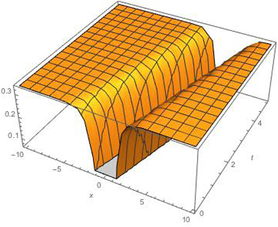
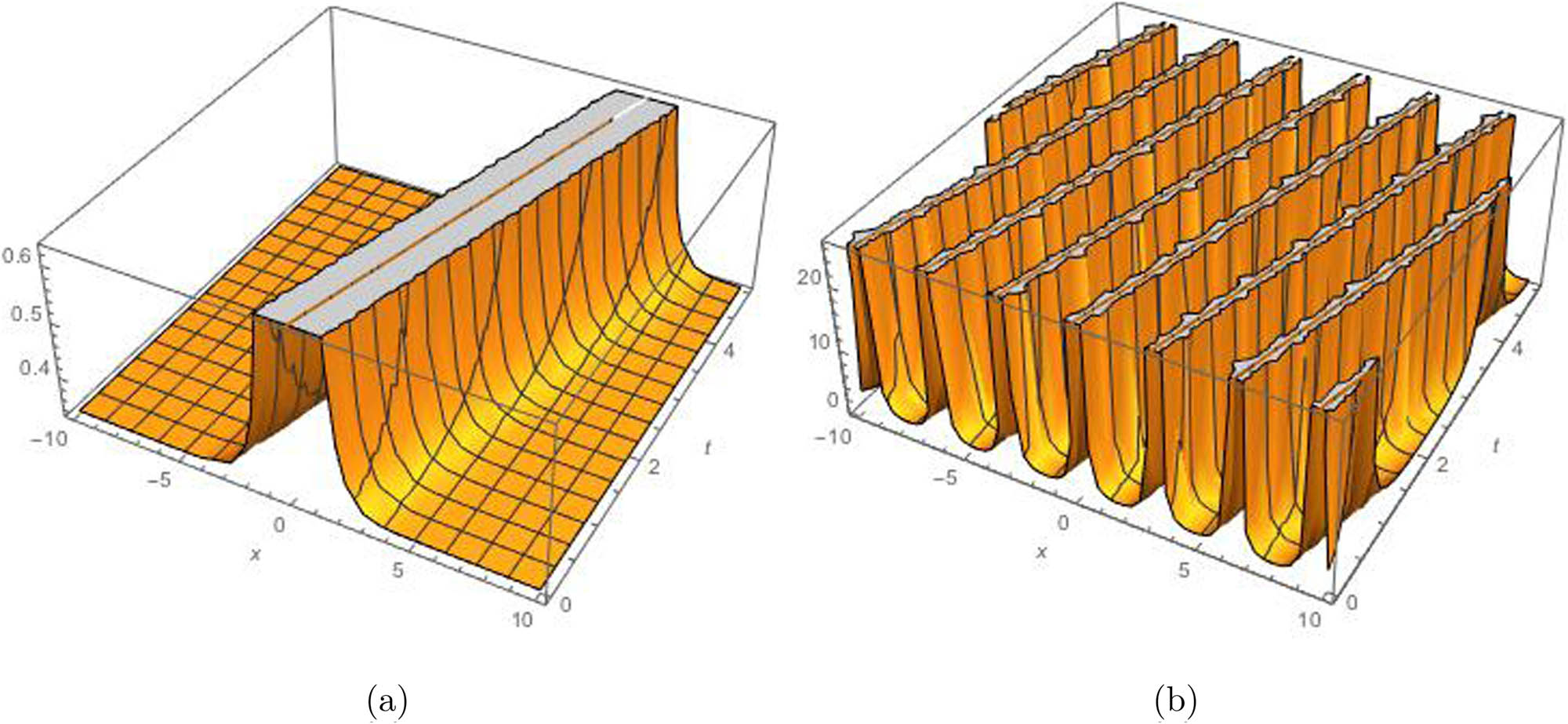
The 3D plot of the solutions (18) when k = 1 .

Case 5. If υ 0 = 1 − k 2 , υ 1 = − 2 − k 2 , and υ 2 = 1 , then Eq. (6) leads to the following solution:

(19) u ( ξ ) = 1 3 ( 2 − k 2 ) + 1 − k 2 cs ( ξ , k ) 2 ,

which can be reduced to

(20) u ( x , t ) = 2 3 + tan 2 ( t − x )

when k → 0 .

Case 6. If υ 0 = 1 , υ 1 = 2 k 2 − 1 , and υ 2 = k 2 ( k 2 − 1 ) , then Eq. (6) admits the following solution:

(21) u ( ξ ) = 1 3 ( 2 k 2 − 1 ) + 1 sd ( ξ , k ) 2 .

Furthermore, the determined solution above converts to:

(22) u ( x , t ) = 1 3 + csch 2 ( t − x )

as k → 1 .

Set 2.

(23) η 0 = 8 υ 1 3 , η 1 = 0 , η 2 = 0 , η − 1 = 0 , η − 2 = 8 υ 0 , c = 176 ( 3 υ 0 υ 2 − υ 1 2 ) .

By substituting previous values into Eq. (9), several cases of analytical solutions are constructed as follows:

Case 1. If υ 0 = 1 , υ 1 = − ( 1 + k 2 ) , and υ 2 = k 2 , then the KK equation in Eq. (8) can be solved as follows:

(24) u ( ξ ) = − 8 3 ( k 2 + 1 ) + 8 sn ( ξ , k ) 2 .

Furthermore, Eq. (24) leads to the following solution:

(25) u ( x , t ) = − 16 3 + 8 coth 2 ( 176 t − x ) ,

(26) u ( x , t ) = − 8 3 + 8 csc 2 ( 176 t − x )

when k → 1 and k → 0 , respectively.

Case 2. If υ 0 = 1 − k 2 , υ 1 = − 2 k 2 − 1 , and υ 2 = − k 2 , then Eq. (6) admits the solution as follows:

(27) u ( ξ ) = 8 3 ( 2 k 2 − 1 ) + 8 ( 1 − k 2 ) cn ( ξ , k ) 2 .

Furthermore, Eq. (14) leads to the following solution:

(28) u ( x , t ) = − 8 3 + 8 sec 2 ( 176 t − x )

when k → 0 .

Case 3. If υ 0 = k 2 − 1 , υ 1 = − 2 − k 2 , and υ 2 = − 1 , then Eq. (6) admits a solution that can be written as follows:

(29) u ( ξ ) = 8 3 ( 2 − k 2 ) + 8 ( k 2 − 1 ) dn ( ξ , k ) 2 .

Case 4. If υ 0 = k 2 , υ 1 = − 1 − k 2 , and υ 2 = 1 , then Eq. (6) satisfies a solution that can be written as follows:

(30) u ( ξ ) = − 8 3 ( k 2 + 1 ) + 8 k 2 ns ( ξ , k ) 2 .

Furthermore, Eq. (30) leads to the following form:

(31) u ( x , t ) = − 16 3 + 8 tanh 2 ( 176 t − x )

when k → 1 .

Case 5. If υ 0 = 1 − k 2 , υ 1 = − 2 − k 2 , and υ 2 = 1 , then Eq. (6) satisfies a solution that can be written as follows:

(32) u ( ξ ) = 8 3 ( 2 − k 2 ) + 8 ( 1 − k 2 ) cs ( ξ , k ) 2 ,

which can be reduced to the following equation:

(33) u ( x , t ) = 16 3 + 8 tan 2 ( 176 t − x )

when k → 0 .

Case 6. If υ 0 = 1 , υ 1 = 2 k 2 − 1 , and υ 2 = k 2 ( k 2 − 1 ) , then, Eq. (6) satisfies the following form:

(34) U ( ξ ) = 8 3 ( 2 k 2 − 1 ) + 8 sd ( ξ , k ) 2 .

Furthermore, the solution determined above transforms to the following equation:

(35) u ( x , t ) = 8 3 + 8 csch 2 ( 176 t − x )

as k → 1 .

Set 3.

(36) η 0 = υ 1 3 , η 1 = 0 , η 2 = υ 2 , η − 1 = 0 , η − 2 = 0 , c = 3 υ 0 υ 2 − υ 1 2 .

By substituting previous values into Eq. (9), several cases of analytical solutions are constructed in the following form:

Case 1. If υ 0 = 1 , υ 1 = − ( 1 + k 2 ) , and υ 2 = k 2 , then the KK equation in Eq. (8) satisfies a solution that can be written as follows:

(37) u ( ξ ) = − 1 3 ( k 2 + 1 ) + k 2 sn ( ξ , k ) 2 .

Case 2. If υ 0 = 1 − k 2 , υ 1 = − 2 k 2 − 1 , and υ 2 = − k 2 , then Eq. (6) admits the solution as follows:

(38) u ( ξ ) = 1 3 ( 2 k 2 − 1 ) − k 2 cn ( ξ , k ) 2 .

Furthermore, the form in Eq. (38) leads to the following solution:

(39) u ( x , t ) = 1 3 − sech 2 ( t − x ) ,

when k → 1 .

Case 3. If υ 0 = k 2 − 1 , υ 1 = − 2 − k 2 , and υ 2 = − 1 , then Eq. (6) satisfies a solution that can be written as follows:

(40) u ( ξ ) = 1 3 ( 2 − k 2 ) − dn ( ξ , k ) 2 .

Case 4. If υ 0 = k 2 , υ 1 = − 1 − k 2 , and υ 2 = 1 , then Eq. (6) satisfies a solution that can be written as follows:

(41) u ( ξ ) = − 1 3 ( k 2 + 1 ) + ns ( ξ , k ) 2 .

Case 5. If υ 0 = 1 − k 2 , υ 1 = − 2 − k 2 , and υ 2 = 1 , then Eq. (6) admits a solution that can be written as follows:

(42) u ( ξ ) = 1 3 ( 2 − k 2 ) + cs ( ξ , k ) 2 ,

which can be reduced to the following form:

(43) u ( x , t ) = 2 3 + cot 2 ( t − x )

when k → 0 .

Case 6. If υ 0 = 1 , υ 1 = 2 k 2 − 1 , and υ 2 = k 2 ( k 2 − 1 ) , then Eq. (6) satisfies a solution that can be written as follows:

(44) u ( ξ ) = 1 3 ( 2 k 2 − 1 ) + k 2 ( k 2 − 1 ) sd ( ξ , k ) 2 .

Set 4.

(45) η 0 = υ 1 3 , η 1 = 0 , η 2 = υ 2 , η − 1 = 0 , η − 2 = υ 0 , c = − 12 υ 0 υ 2 − υ 1 2 .

By substituting previous values into Eq. (9), several cases of exact solutions are constructed in the following forms:

Case 1. If υ 0 = 1 , υ 1 = − ( 1 + k 2 ) , and υ 2 = k 2 , then the KK equation in Eq. (8) satisfies a solution that can be written as follows:

(46) u ( ξ ) = − 1 3 ( k 2 + 1 ) + 1 sn ( ξ , k ) 2 + k 2 sn ( ξ , k ) 2 .

Furthermore, Eq. (11) leads to following form:

(47) u ( x , t ) = − 2 3 + coth 2 ( 16 t − x ) + tanh 2 ( 16 t − x )

when k → 1 .

Case 2. If υ 0 = 1 − k 2 , υ 1 = − 2 k 2 − 1 , and υ 2 = − k 2 , then Eq. (6) admits the following solution:

(48) u ( ξ ) = 1 3 ( 2 k 2 − 1 ) + 1 − k 2 cn ( ξ , k ) 2 + k 2 cn ( ξ , k ) 2 .

Case 3. If υ 0 = k 2 − 1 , υ 1 = − 2 − k 2 , and υ 2 = − 1 , then Eq. (6) admits the following form:

(49) u ( ξ ) = 1 3 ( 2 − k 2 ) + k 2 − 1 dn ( ξ , k ) 2 − dn ( ξ , k ) 2 .

Case 4. If υ 0 = k 2 , υ 1 = − 1 − k 2 , and υ 2 = 1 , then Eq. (6) admits the following form:

(50) u ( ξ ) = − 1 3 ( k 2 + 1 ) + k 2 ns ( ξ , k ) 2 + ns ( ξ , k ) 2 .

Case 5. If υ 0 = 1 − k 2 , υ 1 = − 2 − k 2 , and υ 2 = 1 , then Eq. (6) admits the following form:

(51) u ( ξ ) = 1 3 ( 2 − k 2 ) + 1 − k 2 cs ( ξ , k ) 2 + cs ( ξ , k ) 2 ,

which can be reduced to the following form:

(52) u ( x , t ) = 2 3 + cot 2 ( 16 t − x ) + tan 2 ( 16 t − x )

when k → 0 .

Case 6. If υ 0 = 1 , υ 1 = 2 k 2 − 1 , and υ 2 = k 2 ( k 2 − 1 ) , then Eq. (6) satisfies the following form:

(53) u ( ξ ) = 1 3 ( 2 k 2 − 1 ) + 1 sd ( ξ , k ) 2 + k 2 ( k 2 − 1 ) sd ( ξ , k ) 2 .

Set 5.

(54) η 0 = 8 υ 1 3 , η 1 = 0 , η 2 = 8 υ 2 , η − 1 = 0 , η − 2 = 0 , c = 176 ( 3 υ 0 υ 2 − υ 1 2 ) .

By substituting previous values into Eq. (9), several cases of the following exact solutions can be constructed:

Case 1. If υ 0 = 1 , υ 1 = − ( 1 + k 2 ) , and υ 2 = k 2 , then the KK equation in Eq. (8) admits the following form:

(55) u ( ξ ) = − 8 3 ( k 2 + 1 ) + 8 k 2 sn ( ξ , k ) 2 .

Case 2. If υ 0 = 1 − k 2 , υ 1 = − 2 k 2 − 1 , and υ 2 = − k 2 , then Eq. (6) admits the following solution:

(56) u ( ξ ) = 8 3 ( 2 k 2 − 1 ) − 8 k 2 cn ( ξ , k ) 2 .

Furthermore, Eq. (56) leads to the following form:

(57) u ( x , t ) = 8 3 − 8 sech 2 ( 176 t − x )

when k → 1 .

Case 3. If υ 0 = k 2 − 1 , υ 1 = − 2 − k 2 , and υ 2 = − 1 , then Eq. (6) admits the following solution:

(58) u ( ξ ) = 8 3 ( 2 − k 2 ) − 8 dn ( ξ , k ) 2 .

Case 4. If υ 0 = k 2 , υ 1 = − 1 − k 2 , and υ 2 = 1 , then Eq. (6) satisfies a solution that can be written as follows:

(59) u ( ξ ) = − 8 3 ( k 2 + 1 ) + 8 ns ( ξ , k ) 2 .

Case 5. If υ 0 = 1 − k 2 , υ 1 = − 2 − k 2 , and υ 2 = 1 , then Eq. (6) has a solution of the following form:

(60) u ( ξ ) = 8 3 ( 2 − k 2 ) + 8 cs ( ξ , k ) 2 ,

that can be reduced to the following equation:

(61) u ( x , t ) = 16 3 + 8 cot 2 ( 176 t − x ) ,

when k → 0 .

Case 6. If υ 0 = 1 , υ 1 = 2 k 2 − 1 , and υ 2 = k 2 ( k 2 − 1 ) , then Eq. (6) satisfies the following form of solution:

(62) U ( ξ ) = 8 3 ( 2 k 2 − 1 ) + 8 k 2 ( k 2 − 1 ) sd ( ξ , k ) 2 .

Set 6.

(63) η 0 = 8 υ 1 3 , η 1 = 0 , η 2 = 8 υ 2 , η − 1 = 0 , η − 2 = 8 υ 0 , c = − 176 ( 12 υ 0 υ 2 + υ 1 2 ) .

By substituting previous values into Eq. (9), several cases of the following exact solutions are constructed:

Case 1. If υ 0 = 1 , υ 1 = − ( 1 + k 2 ) , and υ 2 = k 2 , then the KK equation in Eq. (8) satisfies the form of solution as follows:

(64) u ( ξ ) = − 8 3 ( k 2 + 1 ) + 8 sn ( ξ , k ) 2 + 8 k 2 sn ( ξ , k ) 2 .

The solution in Eq. (24) leads to

(65) u ( x , t ) = − 16 3 + 8 coth 2 ( 2816 t − x ) + 8 tanh 2 ( 2816 t − x ) ,

when k → 1 .

Case 2. If υ 0 = 1 − k 2 , υ 1 = − 2 k 2 − 1 , and υ 2 = − k 2 , then Eq. (6) admits the following solution:

(66) u ( ξ ) = 8 3 ( 2 k 2 − 1 ) + 8 ( 1 − k 2 ) cn ( ξ , k ) 2 − 8 k 2 cn ( ξ , k ) 2 .

Case 3. If υ 0 = k 2 − 1 , υ 1 = − 2 − k 2 , and υ 2 = − 1 , then Eq. (6) admits the following solution:

(67) u ( ξ ) = 8 3 ( 2 − k 2 ) + 8 ( k 2 − 1 ) dn ( ξ , k ) 2 − 8 dn ( ξ , k ) 2 .

Case 4. If υ 0 = k 2 , υ 1 = − 1 − k 2 , and υ 2 = 1 , then Eq. (6) admits the following solution:

(68) u ( ξ ) = − 8 3 ( k 2 + 1 ) + 8 k 2 ns ( ξ , k ) 2 + 8 ns ( ξ , k ) 2 .

Case 5. If υ 0 = 1 − k 2 , υ 1 = − 2 − k 2 , and υ 2 = 1 , then Eq. (6) admits the following solution:

(69) u ( ξ ) = 8 3 ( 2 − k 2 ) + 8 ( 1 − k 2 ) cs ( ξ , k ) 2 + 8 cs ( ξ , k ) 2 ,

which can be reduced to:

(70) u ( x , t ) = 16 3 + 8 tan 2 ( 2816 t − x ) + 8 cot 2 ( 2816 t − x ) ,

when k → 0 .

Case 6. If υ 0 = 1 , υ 1 = 2 k 2 − 1 , and υ 2 = k 2 ( k 2 − 1 ) , then Eq. (6) admits the following form of solution:

(71) U ( ξ ) = 8 3 ( 2 k 2 − 1 ) + 8 sd ( ξ , k ) 2 + 8 k 2 ( k 2 − 1 ) sd ( ξ , k ) 2 .

4 Conclusion

In this manuscript, the KK equation has been studied to find new analytical solitary solutions. The MAE method has been utilized to obtain a variety of solutions to the problem under investigation. As far as we know, our solutions are new and different from those in the literature. The obtained solutions are written in terms of Jacobi functions that can be reduced to hyperbolic and trigonometric forms. All solutions obtained in the article have been verified through insertion into the primary equation. Some of the obtained solutions are plotted based on appropriate parameter values. In future work, the analytical methods MAE used in this article can be applied to other types of nonlinear equations for determining the solutions of a suitable model.

Acknowledgments

The author thanks the Dean of Scientific Research at Taif University, Taif, Saudi Arabia, for their support and funding for this work. Moreover, thanks to Dr. Althobaiti for taking the time to provide valuable comments on this article. His suggestions were helpful in accomplishing this work.

Funding information: This work was funded by the Dean of Scientific Research at Taif University, Taif, Saudi Arabia.
Author contributions: All authors have accepted responsibility for the entire content of this manuscript and approved its submission.
Conflict of interest: The author states no conflict of interest.

References

[1] Ezzat MA, El-Bary AA, Morsey MM. Space approach to the hydro-magnetic flow of a dusty fluid through a porous medium. Comput Math Appl. 2010 Apr 1;59(8):2868–79. 10.1016/j.camwa.2010.02.004Suche in Google Scholar

[2] Khater MM, Salama SA. Semi-analytical and numerical simulations of the modified Benjamin-Bona-Mahony model. J Ocean Eng Sci. 2022;7:264–71. 10.1016/j.joes.2021.08.008Suche in Google Scholar

[3] Khan K, Akbar MA, Islam SMR. Exact solution for (1+1)-dimensional nonlinear dispersive modified Benjamin-Bona- Mahony equation and coupled Klein-Gordon equations. Springer Plus. 2014;3, 724; Fractal Fract. 2022;6(399):11 of 11. Suche in Google Scholar

[4] Naher H, Abdullah FA. The modified Benjamin-Bona-Mahony equation via the extended generalized Riccati equation mapping method. Appl Math Sci. 2012;6:5495–512. Suche in Google Scholar

[5] Baskonus HM, Bulut H. Analytical studies on the (1+1)-dimensional nonlinear dispersive modified Benjamin-Bona-Mahony equation defined by seismic sea waves. Waves Random Complex Media. 2015;25:576–86. 10.1080/17455030.2015.1062577Suche in Google Scholar

[6] Che H, Yu-Lan W. Numerical solutions of variable-coefficient fractional-in-space KdV equation with the Caputo fractional derivative. Fractal Fract. 2022;6:207. 10.3390/fractalfract6040207Suche in Google Scholar

[7] Ullah H, Fiza M, Khan I, Alshammari N, Hamadneh NN, Islam S. Modification of the optimal auxiliary function method for solving fractional order KdV equations. Fractal Fract. 2022;6:288. 10.3390/fractalfract6060288Suche in Google Scholar

[8] Ezzat MA, El-Bary AA. Effects of variable thermal conductivity on Stokes’ flow of a thermoelectric fluid with fractional order of heat transfer. Int J Thermal Sci. 2016 Feb 1;100:305–15. 10.1016/j.ijthermalsci.2015.10.008Suche in Google Scholar

[9] Benjamin T, Bona J, Mahony J. Model equations for long waves in nonlinear dispersive systems. Philos Trans R Soc Lond Ser A. 1972;272:47. 10.1098/rsta.1972.0032Suche in Google Scholar

[10] Alotaibi T, Althobaiti A. Exact solutions of the nonlinear modified Benjamin-Bona-Mahony equation by an analytical method. Fractal Fract. 2022;6(7):399. 10.3390/fractalfract6070399Suche in Google Scholar

[11] Parker A. On soliton solutions of the Kaup-Kupershmidt equation. II. ‘Anomalous’ N-soliton solutions. Phys D Nonlinear Phenomena. 2000 Mar 1;137(1-2):34–48. 10.1016/S0167-2789(99)00167-0Suche in Google Scholar

[12] Prakasha DG, Malagi NS, Veeresha P, Prasannakumara BC. An efficient computational technique for time-fractional Kaup-Kupershmidt equation. Numer Meth Partial Differ Equ. 2021 Mar;37(2):1299–316. 10.1002/num.22580Suche in Google Scholar

[13] Sawada K, Kotera T., A method for finding N-soliton solutions of the KdV equation and KdV-like equation. Progress Theoretic Phys. 1974 May 1;51(5):1355–67. 10.1143/PTP.51.1355Suche in Google Scholar

[14] Inc M, Miah M, Akher Chowdhury SA, Rezazadeh H, Akinlar MA, Chu YM. New exact solutions for the Kaup-Kupershmidt equation, Aims Math. 2020 Jan 1;5(6):6726–38. 10.3934/math.2020432Suche in Google Scholar

[15] Kaup DJ. On the inverse scattering problem for cubic eigenvalue problems of the class ψxxx+6Qψx+6Rψ=λψ. Stud Appl Math. 1980 Jun;62(3):189–216. 10.1002/sapm1980623189Suche in Google Scholar

[16] Kupershmidt BA. A super Korteweg-de Vries equation: an integrable system. Phys Lett A. 1984 May 21;102(5–6):213–5. 10.1016/0375-9601(84)90693-5Suche in Google Scholar

[17] Shah NA, Hamed YS, Abualnaja KM, Chung JD, Shah R, Khan A. A comparative analyzis of fractional-order Kaup-Kupershmidt equation within different operators. Symmetry. 2022 May 11;14(5):986. 10.3390/sym14050986Suche in Google Scholar

[18] El-Sayed AA, Agarwal P. Numerical solution of multiterm variable-order fractional differential equations via shifted Legendre polynomials. Math Meth Appl Sci. 2019 Jul 30;42(11):3978–91. 10.1002/mma.5627Suche in Google Scholar

[19] El-Sayed AA, Baleanu D, Agarwal P. A novel Jacobi operational matrix for numerical solution of multi-term variable-order fractional differential equations. J Taibah Univ Sci. 2020 Jan 1;14(1):963–74. 10.1080/16583655.2020.1792681Suche in Google Scholar

[20] Rezapour S, Etemad S, Tellab B, Agarwal P, Garcia Guirao JL. Numerical solutions caused by DGJIM and ADM methods for multi-term fractional BVP involving the generalized ψ-RL-operators. Symmetry. 2021 Mar 25;13(4):532. 10.3390/sym13040532Suche in Google Scholar

[21] Agarwal P, Singh R, ul Rehman A. Numerical solution of hybrid mathematical model of dengue transmission with relapse and memory via Adam-Bashforth-Moulton predictor-corrector scheme. Chaos Solitons Fractals. 2021 Feb 1;143:110564. 10.1016/j.chaos.2020.110564Suche in Google Scholar

[22] Sunarto A, Agarwal P, Sulaiman J, Lung JC. Numerical investigation on the solution of a space-fractional via preconditioned SOR iterative method. Progress Fract Differ Appl. 2022;8(2):289–95. 10.18576/pfda/080208Suche in Google Scholar

[23] Seadawy AR, Rehman SU, Younis M, Rizvi ST, Althobaiti A. On solitons: propagation of shallow water waves for the fifth-order KdV hierarchy integrable equation. Open Physics. 2022 Jan 3;19(1):828–42. 10.1515/phys-2021-0089Suche in Google Scholar

[24] Hereman W, Nuseir A. Symbolic methods to construct exact solutions of nonlinear partial differential equations. Math Comput Simulat. 1997 Jan 1;43(1):13–27. 10.1016/S0378-4754(96)00053-5Suche in Google Scholar

[25] Mahak N, Akram G. The modified auxiliary equation method to investigate solutions of the perturbed nonlinear Schrodinger equation with Kerr law nonlinearity. Optik. 2020;207:164467. 10.1016/j.ijleo.2020.164467Suche in Google Scholar

[26] Althobaiti A. Travelling waves solutions of the KP equation in weakly dispersive media. Open Physics. 2022 Jul 22;20(1):715–23. 10.1515/phys-2022-0053Suche in Google Scholar

[27] Islam R, Alam MN, Hossain AK, Roshid HO, Akbar MA. Traveling wave solutions of nonlinear evolution equations via exp(−ϕ(η))-expansion method. Global J Sci Frontier Res. 2013;13(11):63–71. Suche in Google Scholar

[28] Raslan KR, Khalid KA, Shallal MA. The modified extended tanh method with the Riccati equation for solving the space-time fractional EW and MEW equations. Chaos Solitons Fractals. 2017;103:404–9. 10.1016/j.chaos.2017.06.029Suche in Google Scholar

[29] Gepreel KA, Nofal TA, Althobaiti AA. The modified rational Jacobi elliptic functions method for nonlinear differential difference equations. J Appl Math. 2012;2012:427479. 10.1155/2012/427479Suche in Google Scholar

[30] Althobaiti A, Althobaiti S, El-Rashidy K, Seadawy AR. Exact solutions for the nonlinear extended KdV equation in a stratified shear flow using modified exponential rational method. Results Phys. 2021;29:104723. 10.1016/j.rinp.2021.104723Suche in Google Scholar

[31] Kaewta S, Sirisubtaweee S, Koonprasert S, Sungnul S. Applications of the G’/G2-expansion method for solving certain nonlinear conformable evolution equations. Fractal Fract. 2021;5:88. 10.3390/fractalfract5030088Suche in Google Scholar

[32] Rezazadeh H, Ullah N, Akinyemi L, Shah A, Mirhosseini-Alizamin SM, Chu YM, et al. Optical soliton solutions of the generalized non-autonomous nonlinear Schrödinger equations by the new Kudryashov’s method. Results Phys. 2021;24:104179. 10.1016/j.rinp.2021.104179Suche in Google Scholar

[33] Gepreel KA, Althobaiti AA. Exact solutions of nonlinear partial fractional differential equations using fractional sub-equations method. Indian J Phys. 2014;88(3):293–300. 10.1007/s12648-013-0407-0Suche in Google Scholar

[34] Alotaibi T, Althobaiti A. Exact wave solutions of the nonlinear Rosenau equation using an analytical method. Open Physics. 2021 Dec 31;19(1):889–96. 10.1515/phys-2021-0103Suche in Google Scholar

[35] Banaja MA, Al Qarni AA, Bakodah HO, Zhou Q, Moshokoa SP, Biswas A. The investigate of optical solitons in cascaded system by improved adomian decomposition scheme. Optik. 2017;130:1107–14.10.1016/j.ijleo.2016.11.125Suche in Google Scholar

[36] Alqudah MA, Ashraf R, Rashid S, Singh J, Hammouch Z, Abdeljawad T. Novel numerical investigations of fuzzy Cauchy reaction-diffusion models via generalized fuzzy fractional derivative operators. Fract Fract. 2021;5:151. 10.3390/fractalfract5040151Suche in Google Scholar

[37] Shakhanda R, Goswami P, He J.-H, Althobaiti A. An approximate solution of the time-fractional two-mode coupled Burgers equations. Fract Fract. 2021;5:196. 10.3390/fractalfract5040196Suche in Google Scholar

Received: 2023-05-09

Revised: 2023-08-10

Accepted: 2023-10-14

Published Online: 2023-12-19

This work is licensed under the Creative Commons Attribution 4.0 International License.

Artikel in diesem Heft

https://doi.org/10.1515/phys-2023-0134

Schlagwörter für diesen Artikel

solitary waves; solitons; exact solutions; Jacobi functions; exponential solution

Creative Commons

BY 4.0