Investigation of nanomaterials in flow of non-Newtonian liquid toward a stretchable surface

Lamia Abu El Maati; M. Ijaz Khan; Shaimaa A. M. Abdelmohsen; Badriah M. Alotaibi

doi:10.1515/phys-2023-0171

Article Open Access

Investigation of nanomaterials in flow of non-Newtonian liquid toward a stretchable surface

Lamia Abu El Maati , M. Ijaz Khan , Shaimaa A. M. Abdelmohsen and Badriah M. Alotaibi

Published/Copyright: December 31, 2023

Published by

Become an author with De Gruyter Brill

Submit Manuscript Author Information Explore this Subject

From the journal Open Physics Volume 21 Issue 1

Abstract

This article features the buoyancy-driven electro-magnetohydrodynamic micropolar nanomaterial flow subjected to motile microorganisms. The flow is engendered via an elongating surface, and the energy relation includes heat source generation, magnetohydrodynamics, and radiation. A Buongiorno nanomaterial model (which includes thermophoretic and Brownian diffusions) together with chemical reaction and bioconvection aspects is pondered. The nonlinear governing expressions are transfigured into a dimensionless system, and the dimensionless expressions are computed using the numerical differential-solve scheme. Graphical analyses are conducted to examine the liquid flow, microrotation velocity, microorganism concentration, and temperature in relation to secondary variables. It is observed that a higher Hartman number has an opposite influence on temperature and velocity profiles. A rise in material variables engenders a decline in microrotation velocity. The temperature is enhanced through radiation. The concentration shows conflicting trends for both thermophoretic and random factors. The presence of motile microorganisms reduces the bioconvection Lewis and Peclet numbers.

Keywords: bioconvection; micropolar nanofluid; Ohmic heating; random and thermophoresis diffusions; heat generation and radiation

1 Introduction

In recent times, the inspection of micropolar materials has been remarkable because of its abundant engineering and industrials usages like cervical flows, radial diffusive paint rheology, colloids, and thrust bearing technologies. A micropolar model captures translation along with rotational motions of fluid particles. It has distinct real-world usages in biological fluids and microorganisms (e.g., cilia motion, flagella, and other microorganisms in biological systems), lubrication and bearings (the micropolar model can be applied to evaluate the characteristics of lubricants in bearings and other mechanical components, where the rotational movements of fluid particles play a noteworthy role in the overall fluid dynamics), suspensions and colloidal systems (in suspensions of particles or colloidal systems, the micropolar model can provide insights into the interactions between particles, comprising both translational and rotational aspects), advanced materials processing (understanding micropolar fluid behavior can be beneficial in processes encompassing advanced materials, for illustration composite manufacturing along with additive printing, where the accurate mechanism of fluid flows is essential) and astrophysical fluids (the micropolar model can be utilized in astrophysics to scrutinize the fluid behavior in celestial bodies and space environments). The Naiver–Stokes’ equation that has only a drastic limitation does not adequately describe (by definition) the flow properties for fluids with microstructure. The hypothesis of micropolar material was first given by Eringen [1,2], dealing with fluids that unveil microscopic characteristics appearing from local structure and fundamental motion of liquid elements. The micropolar material is non-Newtonian liquid containing a suspension of small body liquid and colloidal liquid particles like giant dumbbell molecules. Solutal and heat transport analyses for magnetized micropolar liquid flow considering dissipation toward a stretchable wall are elaborated by Saidulu and Reddy [3]. They computed numeric outcomes and found an increment in temperature subjected to higher Eckert number values, while concentration declines with higher Schmidt number values. Kumar et al. [4] investigated the entropy feature for micropolar nanomaterial flow subject to Ohmic heating. They utilized a homotopic scheme for nonlinear analysis. They further reported a rise in angular velocity for the increasing squeezed factor. Magneto-hydrodynamic impact in micropolar nanomaterial flow considering thermal analysis subject to stretchable permeable medium is illuminated by Bilal et al. [5]. They employed the Shooting algorithm for numerical outcomes. Their findings indicate a decline in micro-rotational velocity when the magnetic (Hartman) factor is augmented. Shahzad et al. [6] reported the radiating bioconvective flow of nanomaterial subject to Darcy–Forchheimer rotating disks and generalized heat-mass fluxes. They obtained numeric results through the bvp4c algorithm. The nanoparticle concentration is enlarged when the thermophoresis factor is enlarged. Activation energy characteristics for micropolar material flow featuring varying fluid (viscosity) and thermal (temperature-dependent conductivity) aspects are demonstrated by Saraswathy et al. [7]. They utilized a response surface scheme for solution development. They reported a rise in shear-stress and couple-stress subjected to the increasing viscosity variation factor. Thermal aspects of magnetized flow Williamson micropolar material subject to non-Darcy permeable surface are illustrated by Mishra et al. [8]. They utilized the Runge–Kutta algorithm for computational results. They witnessed a reduction in material velocity against non-Darcian and magnetic factors. Bian et al. [9], Zhang et al. [10], and Yang et al. [11] scrutinized the dynamics of bio-inspired magneto-responsive hybrid type microstructure materials, formulation of a sandwich micro-shell and electromagnetic interference shielding, and electrical performance, respectively. Few important analyses regarding non-Newtonian fluid flow are demonstrated in previous studies [12–15].

A living thing that is so small can be seen only through a microscope. Microorganisms consist of algae, fungi, and bacteria. It helps in processing food digestion, antibiotic development, cleansing environment, farming, nitrogen cycle, and also in the fixation of nitrogen. Bioconvection phenomenon appears due to swimming of motile microorganisms in a liquid. Microorganisms perform incredibly an influential task in the development of pharmaceuticals, engine cooling, agricultural and industrials processes such as biotechnology fields, biofuel, biomedicine, biofertilizers, and bioconvective secondary metabolites. Motile microorganisms have a vital role in biotechnology, medical sciences, micro-systems, micro-fluidic techniques, and many others. One of the most important microorganisms (algae) has the ability to produce more rapid biomass, which can be converted into biodiesel and biofuel [16]. To investigate particular characteristics of these microorganisms in the literature, numerous struggles have been done. Kuznetsov [17] reported the bioconvective flow of nanomaterial containing motile microorganisms considering random and thermophoretic diffusions. He acquired perturbed solutions for nonlinear mathematical expressions and declared that the presence of nanoparticles upsurges the critical Rayleigh factor by a considerable quantity. Avramenko et al. [18] illustrated the magnetized bioconvective flow of viscous liquid including motile microorganisms. They used a Lorenz procedure and reported the bioconvective flow instability. According to them, when the Schmidt number exceeds 8, then variations in viscosity or diffusion exert a more pronounced influence on the oscillations than the microorganism-specific shape. An impact of the Marangoni convective radiating flow of the Williamson nanoliquid containing microorganisms subjected to moving surface is illustrated by Kairi et al. [19]. They applied the Runge–Kutta–Fehlberg algorithm and computed numeric outcomes. They noted a decline in heat–mass transfer rates when the material variable is enlarged. Aziz et al. [20] highlighted features of motile microorganisms with the suspension of nanoparticles in the viscous fluid flow. They computed numerical results and reported that the buoyancy factor has a noteworthy influence on dimensionless physical quantities. Ghachem et al. [21] highlighted features of heat source in bio-convective dissipative flow of nanoliquid considering convective condition. Here, the nonlinear expressions are computed numerically through the shooting scheme. The consideration of convective along with slip boundary constraints effectually improved the transference phenomenon. Zhang et al. [22] examined micro-structural and mechanical characteristics of alkali-activated nanocomposites. Xu et al. [23], Zheng et al. [24], and Hu et al. [25] recently explored the behavior of bio-mimetic nanomaterials as fluorescent sensors, dielectric barrier discharge plasma actuator, and hybrid liquid flow with the multiphysics coupling model. Few important investigations about gyrotactic microorganism and other flow assumptions are presented in previous studies [26–31].

Nanofluids are deployed to intensify the thermal transportation phenomenon of base liquid that leads to enhance the heat transfer coefficient. They have many biomedical and engineering applications in cancer therapy, cooling industry, and process industry. Enhancement in thermal conductivity increases the performance of thermal systems. In some cases, specific heat capacity of nanofluid declines with the addition of nanoparticles in the base fluid. Nanofluids represent those fluids that contains nanometer-sized particles. The nanoparticles have exceptionally smaller size or similar to coherent or de Brogile waves. Due to this phenomenon, nanoparticles exhibit behaviors akin to energy materials. Their size should be in the range of 1–100 nm. These particles are utilized to upsurge or decline the heat transference. In recent times, scientists have been increasingly captivated by nanoliquids owing to their crucial thermal properties. Enhancing the thermal efficiency of their transport stands is one of the several applications of such substances. Nanoliquids can be applied in vehicle cooling, nanowires, artificial intelligence, fuel cells, radiotherapy, brain tumors, inorganic lungs, nanofibers, surgery, pharmaceutical processes, engine cooling, electronic chilling system, cancer therapy, domestic refrigerators, and radiators. Choi et al. [32,33] introduced the concept of nanofluids. In his work, he delved into the nanomaterial thermal conductivity. Buongiorno [34] presented the concept of thermal conduction improvement of liquid. The Buongiorno model offers a comprehensive framework to study the behavior of nanofluids by considering interactions between the base materials and dispersed nanoparticles. It provides insights into heat transfer and fluid dynamics in nanofluid-based systems, impacting a range of practical applications. Kalpana et al. [35] highlighted the magnetohydrodynamic time-dependent flow of the nanomaterial subject to thermophoresis and random diffusions. They utilized the finite difference algorithm, quasilinear approach, and Thomas scheme for simulation. Significant findings reveal that increasing the wavy wall amplitude has a noticeable impact on flow. Few related studies regarding nanofluid are presented in previous studies [36–45].

In this study, the subsequent dimensionless couple systems are calculated numerically via numerical differential (ND)-solve technique. Features of liquid flow, concentration, microrotation velocity, motile microorganisms, and temperature against emerging variables are graphically analyzed.

2 Constitutive relations

The fundamental expressions governing the micropolar fluid are as follows [46]:

(1) d i v V = 0 ,

(2) ρ f d V d t = d i v T ,

(3) ρ f j d Ω d t = d i v M + ε 1 ,

(4) T = λ 1 ∗ ( tr A 1 ) I + 2 μ A 1 + 2 k ∗ ε 1 ⋅ ( ω − Ω ) ,

(5) M = α ν ( ∇ ⋅ Ω ) I + β ν ( ∇ Ω ) tr + γ ν ∇ Ω ,

(6) A 1 = 1 2 [ g r a d V + ( g r a d V ) tr ] ,

(7) ω = 1 2 ( ∇ × V ) ,

(8) V = [ u ( x , y ) , v ( x , y ) , 0 ] ,

(9) Ω = [ 0 , N ( x , y ) , 0 ] ,

where ( M , T ) represents (couple-stress, stress) tensor, ( V , ω ) represents (velocity, vorticity) vector, ρ f is the nanofluid density, Ω is the angular velocity representing fluid particles micro-motion, j is micro-inertia, ε 1 is third-rank tensor, ( k ∗ , λ 1 ∗ , μ ) is the (vortex, bulk, shear) viscosity, I represents volume coupling force, and ( α ν , β ν , γ ν ) represents spin viscosities.

The aforementioned expressions yield [46]:

(10) ∂ u ∂ x + ∂ v ∂ y = 0 ,

(11) u ∂ u ∂ x + v ∂ u ∂ y = ν + k ∗ ρ f ∂ 2 u ∂ y 2 + k ∗ ρ f ∂ N ∂ y ,

(12) u ∂ N ∂ x + v ∂ N ∂ y = γ ν ρ f j ∂ 2 N ∂ y 2 − k ∗ ρ f 2 N + ∂ u ∂ y .

3 Formulation

Here, electromagnetohydrodynamics two-dimensional bioconvection flow of micropolar nanomaterial containing microorganisms toward a stretched wall is considered. Boungiorno’s model is deployed to inspect the nanofluid significance by thermophoretic and random diffusions. Heat generation, chemical reaction, Ohmic heating, and radiation are taken into account. Uniform electric ( E 0 ) and magnetic ( B 0 ) fields are applied. Moving surface has velocity u = u w = a x (in which a is the rate constant). The micropolar nanoliquid is expected to exist as a diluted suspension subjected to a uniform distribution of gyrotactic microorganisms. The stability of suspension certifies that nanoparticles do not agglomerate. It is important to mention that the presence of nanoparticles does not influence the swimming velocity or the direction of gyrotactic microorganisms when the nanoparticle concentration remains below 1%. The bioconvection effects turn out to be significant under lower adjourned nanoparticle concentrations. The diffusing species concentration in binary concoction is considered significantly smaller compared to the other existing species. As a result, the Soret–Dufour aspects can be overlooked, and the temperature within the flowing fluid is primarily determined by the energy concentration expression, which includes radiative heat considerations. Figure 1 elucidates the flow configuration.

Figure 1

Schematic flow analysis.

The related equations subjected to considered rheological characteristics are as follows [47]:

(13) ∂ u ∂ x + ∂ v ∂ y = 0 ,

(14) u ∂ u ∂ x + v ∂ u ∂ y = μ + k ρ f ∂ 2 u ∂ y 2 + k ρ f ∂ N ∂ y + σ f ρ f ( E 0 B 0 − B 0 2 u ) 1 ρ f g ρ f β ∗ ( 1 − C ∞ ) ( T − T ∞ ) − g ( ρ p − ρ f ) ( C − C ∞ ) − γ 1 g ( ρ m − ρ f ) ( n − n ∞ ) ,

(15) u ∂ N ∂ x + v ∂ N ∂ y = γ ∗ ρ j ∂ 2 N ∂ y 2 − k ρ j 2 N + ∂ u ∂ y ,

(16) u ∂ T ∂ x + v ∂ T ∂ y = α 1 ∂ 2 T ∂ y 2 + τ D B ∂ T ∂ y ∂ C ∂ y + D T T ∞ ∂ T ∂ y 2 + σ f ( ρ c p ) f ( u B 0 − E 0 ) 2 + Q 0 ( ρ c p ) f ( T − T ∞ ) + 16 σ ∗ T ∞ 3 3 k ∗ ( ρ c p ) f ∂ 2 T ∂ y 2 ,

(17) u ∂ C ∂ x + v ∂ C ∂ y = D B ∂ 2 C ∂ y 2 + D T T ∞ ∂ 2 T ∂ y 2 − k r ( C − C ∞ ) ,

(18) u ∂ n ∂ x + v ∂ n ∂ y + b W C ( C w − C ∞ ) ∂ ∂ y n ∂ C ∂ y = D m ∂ 2 n ∂ y 2 ,

with the following conditions [47]:

(19) u = a x , v = 0 , N = − m 0 ∂ u ∂ y , T = T w , C = C w , n = n w at y = 0 u → 0 , N → 0 , T → T ∞ , C → C ∞ , n → n ∞ , as y → ∞ .

Here, ( u , v ) are the velocity components, ν f is the kinematic viscosity, ( x , y ) is the Cartesian coordinate, g is the gravity, σ f is the electrical conductivity, ( k , γ ∗ ) are vortex and spin-gradient viscosities, respectively, j is the micro inertia, k f is the thermal conductivity, β ∗ is the volume expansion coefficient, T is the temperature, σ ∗ is the Stefan–Boltzmann constant, N is the micro-rotation velocity, ρ f is density, D T is the thermophoresis coefficient, Q 0 is heat-generation coefficient, m 0 is the boundary variable, D B is the Brownian–diffusion coefficient, α f is thermal diffusivity, D m is the swimming microorganism coefficient, τ is the ratio of heat capacitance, c p is specific heat, k ∗ is the mean-absorption coefficient, ( T ∞ , n ∞ , C ∞ ) are ambient temperature, microorganism concentration, and concentration, respectively, n is the concentration of microorganisms, W C is cell swimming speed, k r is the reaction rate, b is the chemotaxis constant, and ( T w , n w , C w ) are the wall temperature, microorganism concentration, and concentration, respectively.

Letting [47]:

(20) u = a x f ′ ( η ) , v = − a ν f f ( η ) , θ ( ξ , η ) = T − T ∞ T w − T ∞ , ϕ ( η ) = C − C ∞ C w − C ∞ ξ ( η ) = n − n ∞ n w − n ∞ , N = a x a ν f g , η = a ν f y .

Finally, we have

(21) ( 1 + K ) f ‴ − f f ″ − f ′ 2 + K g ′ + Ha ( E − f ′ ) + λ ( θ − β 1 ϕ − β 2 ξ ) = 0 ,

(22) 1 + K 2 g ″ − f ′ g + g ′ f − K ( 2 g + f ″ ) = 0 ,

(23) ( 1 + Rd ) θ ″ + Pr f θ ′ + Pr HaEc ( f ′ − E ) 2 + Pr Nb θ ′ ϕ ′ + Pr Nt θ ′ 2 + Pr Q θ = 0 ,

(24) ϕ ″ + Sc f ϕ ′ + Nt Nb θ ″ − Sc γ ϕ = 0 ,

(25) ξ ″ + Lb f ξ − Pe [ ϕ ″ ( Ω + ξ ) + ξ ′ ϕ ′ ] = 0 ,

(26) f ′ ( 0 ) = 1 , f ( 0 ) = 0 , g ( 0 ) = − m 0 f ″ ( 0 ) , θ ( 0 ) = 1 , ϕ ( 0 ) = 1 , ξ ( 0 ) = 1 f ′ ( ∞ ) = 0 , g ( ∞ ) = 0 , θ ( ∞ ) = 0 , ϕ ( ∞ ) = 0 , ξ ( ∞ ) = 0 .

In the aforementioned expressions, Ha = σ f B 0 2 a ρ f is the Hartman number, K = k μ f is the material parameter, Nt = τ D T ( T w − T ∞ ) ν f T ∞ is the thermophoresis variable, E = E 0 u w B 0 is the electric field variable, Pe = b W C D m is the Peclet number, λ = g β ∗ ( 1 − C ∞ ) ( T w − T ∞ ) a ρ f is the mixed convection factor, Rd = 16 σ ∗ T ∞ 3 3 k ∗ k f is the radiative variable, Pr = ν f α f is the Prandtl number, Nb = τ D B ( C w − C ∞ ) ν f is the Brownian diffusion factor, Ec = u 0 2 c p ( T w − T ∞ ) is the Eckert number, β 1 = ( ρ p − ρ f ) ( C w − C ∞ ) g β ∗ ( 1 − C ∞ ) ( T w − T ∞ ) is the buoyancy ratio variable, Q = Q 0 a ( ρ c p ) f is the thermal-generation variable, β 2 = γ 1 ( ρ m − ρ f ) ( n w − n ∞ ) g β ∗ ( 1 − C ∞ ) ( T w − T ∞ ) is the bioconvection Rayleigh number, γ = k r a is the reactive variable, Lb = ν f D m is the bioconvective Lewis number, and Ω = n ∞ ( n w − n ∞ ) is the microorganism difference factor.

4 Engineering quantities

4.1 Heat transference rate (Nusselt number)

The heat-transference rate is given by [38]:

(27) Nu x = x q w k f ( T w − T ∞ ) ,

where heat flux ( q w ) is expressed as follows:

(28) q w = − k f + 16 σ ∗ T ∞ 3 3 k ∗ ∂ T ∂ y y = 0 .

A dimensionless form is given by

(29) Nu x R e x − 1 / 2 = − ( 1 + Rd ) θ ′ ( 0 ) .

4.2 Mass transference rate (Sherwood number)

The Sherwood number is given by [38]:

(30) Sh x = x j w D B ( C w − C ∞ ) .

The mass flux ( j w ) obeys the following equation:

(31) j w = − D B ∂ C ∂ y y = 0 .

A nondimensional form is given by

(32) Sh x R e x − 1 / 2 = − ϕ ′ ( 0 ) .

5 Numerical computation

This section provides an overview of the numerical techniques used in this study. The computational approach employed in this investigation utilizes the ND-solve method, a boundary value problem solver implemented in MATHEMATICA. This method, also known as the “Shooting” method, is specifically designed for solving various flow problems (e.g., Navier–Stokes expressions) under distinct conditions. The governing mathematical expressions expressed in a nondimensional mathematical form are developed from Navier–Stokes expressions. To effectually compute such nonlinear expressions, the “shooting” method employs a series of carefully selected similarity transformations. These transformations allow for the manipulation and the solution of governing flow rheological expressions in a more efficient manner.

In this study, a crucial step in the transformation process involves converting the coupled systems (i.e., Eqs. (21)–(26)) into first-order mathematical systems via transformations. This conversion from higher-order mathematical expressions to first-order mathematical one simplifies the problem and makes it more well suited with the deployed numerical schemes. The interpretation of these novel transformational mathematical systems is described in detail below.

(33) f = z 1 , f ′ = z 2 , f ″ = z 3 , f ‴ = Z 11 g = z 4 , g ' = z 5 , g ' ' = Z 22 θ = z 6 , θ ' = z 7 , θ ' ' = Z 33 ϕ = z 8 , ϕ ' = z 9 , ϕ ' ' = Z 44 ξ = z 10 , ξ ' = z 11 , ξ ' ' = Z 55 ,

(34) Z 11 = 1 ( 1 + K ) [ z 1 z 3 + z 2 2 − K z 5 − Ha ( E − z 2 ) − λ ( z 6 − β 1 z 8 − β 2 z 10 ) ] ,

(35) Z 22 = 1 1 + K 2 [ z 1 z 5 − z 2 z 4 + K ( 2 z 4 + z 3 ) ] ,

(36) Z 33 = − 1 1 + Rd [ Pr z 1 z 6 + Pr HaEc ( z 2 − E ) 2 + Pr Nb z 7 z 9 + Pr Nt z 7 2 + Pr Q z 6 ] ,

(37) Z 44 = − 1 Sc z 1 z 9 + Nt Nb Z 33 − Sc γ Z 8 ,

(38) Z 55 = − 1 Lb [ z 1 z 10 − Pe ( Z 44 ( Ω + z 10 ) + z 11 z 9 ) ] ,

with

(39) z 1 ( 0 ) = 0 , z 2 ( 0 ) = 1 , z 4 ( 0 ) = − m 0 z 3 ( 0 ) , z 6 ( 0 ) = z 8 ( 0 ) = z 10 ( 0 ) = 1 z 2 ( ∞ ) = 0 , z 4 ( ∞ ) = 0 , z 6 ( ∞ ) = 0 , z 8 ( ∞ ) = 0 , z 10 ( ∞ ) = 0 .

6 Analysis

This section elaborates nondimensional parameters impact on dimensionless parameters such as velocity f ′ ( η ) , microrotation velocity ( g ( η ) ) , temperature ( θ ( η ) ) , concentration ( ϕ ( η ) ) , and motile microorganisms ( ξ ( η ) ) . These parameters are plotted in Figures 2–15.

$Figure 2 f ′ ( η ) f^{\prime} (\eta ) via E E .$

Figure 2

f ′ ( η ) via E .

$Figure 3 f ′ ( η ) f^{\prime} (\eta ) via Ha \text{Ha} .$

Figure 3

f ′ ( η ) via Ha .

$Figure 4 f ′ ( η ) f^{\prime} (\eta ) via K K .$

Figure 4

f ′ ( η ) via K .

$Figure 5 f ′ ( η ) f^{\prime} (\eta ) via λ \lambda .$

Figure 5

f ′ ( η ) via λ .

$Figure 6 g ( η ) g(\eta ) via m 0 {m}_{0} .$

Figure 6

g ( η ) via m 0 .

$Figure 7 θ ( η ) \theta (\eta ) via Ha \text{Ha} .$

Figure 7

θ ( η ) via Ha .

$Figure 8 θ ( η ) \theta (\eta ) via Nt \text{Nt} .$

Figure 8

θ ( η ) via Nt .

$Figure 9 θ ( η ) \theta (\eta ) via Pr \Pr .$

Figure 9

θ ( η ) via Pr .

$Figure 10 θ ( η ) \theta (\eta ) via Rd \text{Rd} .$

Figure 10

θ ( η ) via Rd .

$Figure 11 ϕ ( η ) \phi (\eta ) via γ \gamma .$

Figure 11

ϕ ( η ) via γ .

$Figure 12 ϕ ( η ) \phi (\eta ) via Sc \text{Sc} .$

Figure 12

ϕ ( η ) via Sc .

$Figure 13 ξ ( η ) \xi (\eta ) via Ω \Omega .$

Figure 13

ξ ( η ) via Ω .

$Figure 14 ξ ( η ) \xi (\eta ) via Pe \text{Pe} .$

Figure 14

ξ ( η ) via Pe .

$Figure 15 ξ ( η ) \xi (\eta ) via Lb \text{Lb} .$

Figure 15

ξ ( η ) via Lb .

The electric field ( E ) characteristics versus velocity f ′ ( η ) are explained in Figure 2. Physically increasing values of the electric field leads to upsurge the velocity field. This relationship is a vital characteristic of electromagnetism, where a sturdier electric field utilizes greater force on charged elements, accelerating them and subsequently improving the velocity field. This phenomenon is usually witnessed in numerous physical systems and plays a crucial role in comprehension and deploying electrical and electromagnetic procedures. Figure 3 reports the velocity variation against the Hartmann number ( Ha ) . Due to increasing Lorentzian forces, a decay in velocity is evidently observed subjected to higher Hartmann number. The observed phenomenon suggests that the Lorentz forces, resulting from the interaction between electric currents and magnetic fields, serve to restrict the velocity within the system as the Hartmann number (which quantifies the strength of the magnetic field) increases. Figure 4 shows the material ( K ) variable effects against f ′ ( η ) . An increment occurs in the fluid flow for higher material parameter. Physically when viscosity upsurges, the resistance to the liquid flow rises as well. Consequently, it necessitates extra force or energy to propel the liquid, leading to heightened liquid motion. Figure 5 depicts thermal convection variation ( λ ) variations versus f ′ ( η ) . There is an enhancement of velocity against ( λ ) . The convection factor describes the balance between forced convection (persuaded by external forces) and natural convection (driven by thermal gradients). When λ increases, it implies a more noticeable effect of forced convection, which characteristically leads to augmented fluid velocity as external forces have a sturdier influence on the flow. Figure 6 explains the effect of ( m 0 ) on microrotation velocity ( g ( η ) ) . The maximum values of ( m 0 ) boost the microrotation velocity. The fluid unveils a more significant response to the influencing factors or conditions, representing a sensitivity of fluid’s behavior subjected to increasing ( m 0 ) . Figure 7 portrays the impact of Hartmann ( Ha ) number on temperature ( θ ( η ) ) . Clearly, the thermal field is the enhancing function of Hartmann number. Without a doubt, the larger Hartmann ( Ha ) number leads to greater Lorentzian resistive force within the system. This, in turn, results in elevated temperatures. The relationship between ( Ha ) and the Lorentzian resistive force implies that higher ( Ha ) values augment the resistive features of magnetic forces on the fluid, causing more noteworthy heating and contributing to higher temperatures within the system. Characteristic of thermal filed subject to thermophoresis ( Nt ) parameter is reported in Figure 8. Higher approximation of thermophoresis and Brownian motion variable leads to the increased thermal distribution. The increasing Brownian diffusion factor leads to an instantaneous and more erratic random particle movement, eventually yielding higher temperature. Furthermore, the thermophoresis phenomenon comprises the particle movement from hotter toward cooler. This movement of fluid particles yields an elevation in the nanofluid temperature. Figure 9 displays the Prandtl number variation on θ ( η ) . Physically rising values of Prandtl ( Pr ) number leads to reduction in the thermal diffusivity and consequently a decline in temperature. This phenomenon transpires because a higher Prandtl ( Pr ) number implies a sturdier dominance of momentum diffusion over thermal diffusion. Therefore, heat is transported less competently, causing the temperature to diminution due to reduced diffusivity. Figure 10 depicts the influence of radiation variable ( Rd ) against temperature. It shows that the rising values of the radiation variable intensify the thermal field. In other words, as the radiation variable ( Rd ) turns out to be larger, it applies a greater impact on the thermal aspects of system, leading to an enhancement in the thermal field. Figure 11 elaborates the effect of reaction variable ( γ ) on concentration ( ϕ ( η ) ) . It is obvious from the figure that as γ rises, the concentration ( ϕ ( η ) ) declines. This reveals a strong inverse relationship between γ and ϕ ( η ) , signifying that a larger γ leads to a decrease in ϕ ( η ) . Figure 12 reveals the impact of the Schmidt number ( Sc ) on the concentration profile. The concentration distribution decreases as the Schmidt number increased. This means that as the Schmidt number (which describes the relationship between momentum and mass diffusion) becomes larger, the concentration distribution diminishes. The graphical explanation of ( Ω ) on ( ξ ( η ) ) is shown in Figure 13. Motile microorganisms reduce with higher approximation of ( Ω ) . In fact, larger Ω produces a larger disparity between the density of microorganisms at plate surface and the ambient density of microorganisms. This disparity inspires the concentration of motile microorganisms. In simpler terms, as Ω upsurges, the difference in microorganism density near the plate and in the surrounding environment turns out to be more noticeable, which, in turn, stimulates the concentration of motile microorganisms near the plate surface. The effects of Peclet and bioconvective Lewis ( Lb ) numbers are shown in Figures 14 and 15. Here, the microorganism field ( ξ ( η ) ) decays for higher Peclet and Lewis numbers. Physically, the increasing Peclet number engenders a decline in density of motile microorganisms, which corresponds to lower concentration. In addition, the concentration of motile microorganisms diminishes when Lb is augmented. Such a trend is found because swimming microorganism coefficient ( D m ) reduces when Lb is increased.

Table 1 exhibits a comparative study about results acquired here with those from the research of Waqas et al. [43], and it is evident that the obtained results are in strong agreement. Such agreement between independent studies enhances the reliability and validity of the utilized methodology.

Table 1

Comparative outcomes of − C fx Re x − 1 2 for distinct estimations of Ha

Ha	Waqas et al. [43]	Current study
0.0	−1.00000	−1.00000
0.5	−1.1180	−1.11803
1.0	−1.4141	−1.41421

7 Closing remarks

The present analysis has provided several key findings:

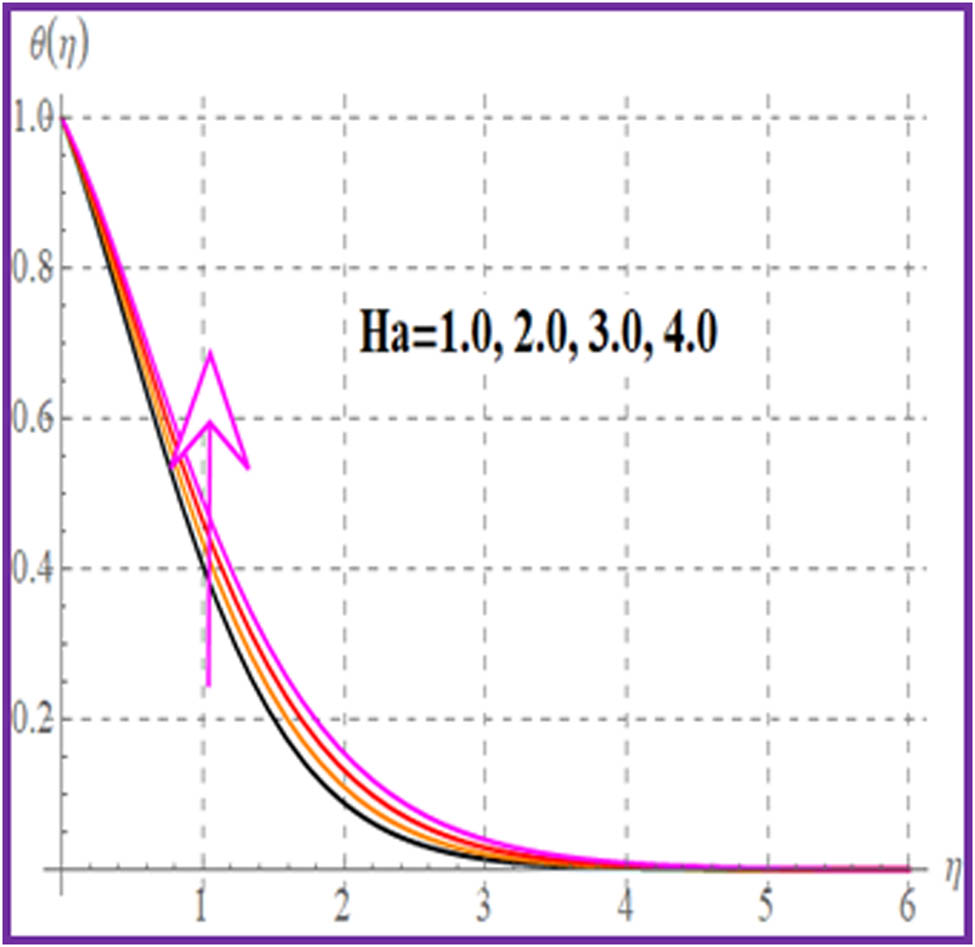
Fluid flow decays as the Hartmann number increases, while the reverse trend is observed for temperature.
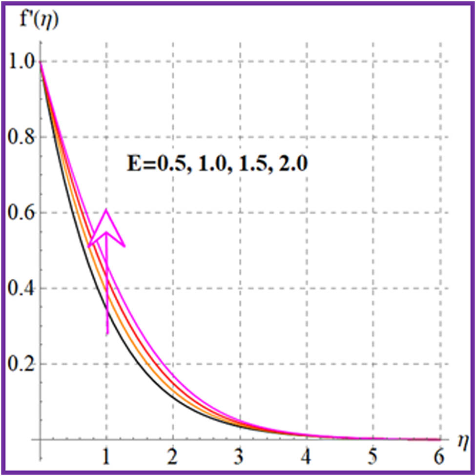
A larger estimation of the electric field variable enhances the velocity.
Higher material variables lead to a reverse behavior in fluid flow and microrotation velocity.
Microrotation velocity increases against an unknown variable.
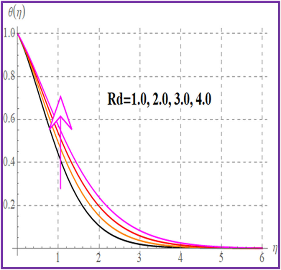
Temperature exhibits opposite behavior for larger radiation and Prandtl numbers.
The thermal field shows an increasing behavior with random and thermophoresis variables.
An increase in concentration is observed against the thermophoresis variable.
Variation in the Schmidt number yields concentration reduction.
Concentration decreases for Brownian and thermophoresis variables.
Motile microorganisms decay for higher unknown variable.
Motile microorganisms shrink against higher Peclet numbers.
Variation in the bioconvective Lewis number engenders a decline in motile microorganisms.

These findings provide useful understandings regarding fluid flow, temperature, microrotation velocity, concentration, and motile microorganisms under different variables. Further research can be conducted to explore the underlying mechanisms and extend the analysis to more complex systems.

Acknowledgments

The authors extend their appreciation to the Deputyship for Research & Innovation, Ministry of Education in Saudi Arabia for funding this research work through the project number RI-44-0332.

Funding information: The authors extend their appreciation to the Deputyship for Research & Innovation, Ministry of Education in Saudi Arabia for funding this research work through the project number RI-44-0332.
Author contributions: All authors have accepted responsibility for the entire content of this manuscript and approved its submission.
Conflict of interest: The authors state no conflict of interest.

References

[1] Eringen AC. Simple microfluids. Int J Eng Sci. 1964;2:205–17.10.1016/0020-7225(64)90005-9Search in Google Scholar

[2] Eringen AC. Theory of micropolar fluids. J Math Mech. 1966;16:1–18.10.1512/iumj.1967.16.16001Search in Google Scholar

[3] Saidulu B, Reddy KS. Evaluation of combined heat and mass transfer in hydromagnetic micropolar flow along a stretching sheet when viscous dissipation and chemical reaction is present. Partial Differ Equ Appl Math. 2023;7:100467. 10.1016/j.padiff.2022.100467.Search in Google Scholar

[4] Kumar NN, Sastry DRVSRK, Shaw S. Irreversibility analysis of an unsteady micropolar CNT-blood nanofluid flow through a squeezing channel with activation energy-Application in drug delivery. Comput Methods Prog Biomed. 2022;226:107156. 10.1016/j.cmpb.2022.107156.Search in Google Scholar PubMed

[5] Bilal M, Ramzan M, Siddique I, Sajjad A. Magneto-micropolar nanofluid flow through the convective permeable channel using Koo-Kleinstreuer-Li model. J Magn Magn Mater. 2023;565:170288. 10.1016/j.jmmm.2022.170288.Search in Google Scholar

[6] Shahzad A, Imran M, Tahir M, Khan SA, Akgül A, Abdullaev S, et al. Brownian motion and thermophoretic diffusion impact on Darcy-Forchheimer flow of bioconvective micropolar nanofluid between double disks with Cattaneo-Christov heat flux. Alex Eng J. 2023;62:1–15.10.1016/j.aej.2022.07.023Search in Google Scholar

[7] Saraswathy M, Prakash D, Muthtamilselvan M, Mdallal QMA. Arrhenius energy on asymmetric flow and heat transfer of micropolar fluids with variable properties: A sensitivity approach. Alex Eng J. 2022;61:12329–52.10.1016/j.aej.2022.06.015Search in Google Scholar

[8] Mishra P, Kumar D, Kumar J, Aty AHA, Park C, Yahia IS. Analysis of MHD Williamson micropolar fluid flow in non-Darcian porous media with variable thermal conductivity. Case Stud Therm Eng. 2022;36:102195. 10.1016/j.csite.2022.102195.Search in Google Scholar

[9] Bian Y, Zhu S, Li X, Tao Y, Nian C, Zhang C, et al. Bioinspired magnetism-responsive hybrid microstructures with dynamic switching toward liquid droplet rolling states. Nanoscale. 2023;15:11945–54.10.1039/D3NR02082GSearch in Google Scholar PubMed

[10] Zhang M, Jiang X, Arefi M. Dynamic formulation of a sandwich microshell considering modified couple stress and thickness-stretching. Eur Phys J Plus. 2023;138:227.10.1140/epjp/s13360-023-03753-4Search in Google Scholar

[11] Yang B, Wang H, Zhang M, Jia F, Liu Y, Lu Z. Mechanically strong, flexible, and flame-retardant Ti3C2Tx MXene-coated aramid paper with superior electromagnetic interference shielding and electrical heating performance. Chem Eng J. 2023;476:146834.10.1016/j.cej.2023.146834Search in Google Scholar

[12] Fares ME, Salem MG, Atta D, Elmarghany MK. Mixed variational principle for micropolar elasticity and an accurate two-dimensional plate model. Eur J Mech A Solids. 2023;99:104870. 10.1016/j.euromechsol.2022.104870.Search in Google Scholar

[13] Shabbir T, Mushtaq M, Khan MI, Hayat T. Modeling and numerical simulation of micropolar fluid over a curved surface: Keller box method. Comput Methods Prog Biomed. 2022;187:105220. 10.1016/j.cmpb.2019.105220.Search in Google Scholar PubMed

[14] Faisal M, Mabood F, Asogwa KK, Badruddin IA. Bidirectional radiative transport of magnetic Maxwell nanofluid mobilized by Arrhenius energy and prescribed thermal/concentration conditions: Significance of Ludwig-Soret and pedesis effects. Ain Shams Eng J. 2023;14:101933.10.1016/j.asej.2022.101933Search in Google Scholar

[15] Waqas M, Sadiq MA, Bahaidarah HMS. Gyrotactic bioconvection stratified flow of magnetized micropolar nanoliquid configured by stretchable radiating surface with Joule heating and viscous dissipation. Int Commun Heat Mass Transf. 2022;138:106229. 10.1016/j.icheatmasstransfer.2022.106229.Search in Google Scholar

[16] Singh SP, Singh P. Effect of temperature and light on the growth of algae species: A review. Renew Sustain Energy Rev. 2015;50:431–44.10.1016/j.rser.2015.05.024Search in Google Scholar

[17] Kuznetsov AV. The onset of nanofluid bioconvection in a suspension containing both nanoparticles and gyrotactic microorganisms. Int Commun Heat Mass Trans. 2010;37:1421–5.10.1016/j.icheatmasstransfer.2010.08.015Search in Google Scholar

[18] Avramenko AA, Kovetska YY, Shevchuk IV. Lorenz approach for analysis of bioconvection instability of gyrotactic motile microorganisms. Chaos Solit Fractals. 2023;166:112957. 10.1016/j.chaos.2022.112957.Search in Google Scholar

[19] Kairi RR, Roy S, Raut S. Stratified thermosolutal Marangoni bioconvective flow of gyrotactic microorganisms in Williamson nanofluid. Eur J Mech B/Fluids. 2023;97:40–52.10.1016/j.euromechflu.2022.09.004Search in Google Scholar

[20] Aziz A, Khan WA, Pop I. Free convection boundary layer flow past a horizontal flat plate embedded in porous mediumfilled by nanofluid containing gyrotactic microorganisms. Int J Therm Sci. 2012;56:48–57.10.1016/j.ijthermalsci.2012.01.011Search in Google Scholar

[21] Ghachem K, Ahmad B, Noor S, Abbas T, Khan SU, Anjum S, et al. Numerical simulations for radiated bioconvection flow of nanoparticles with viscous dissipation and exponential heat source. J Indian Chem Soc. 2023;100(1):100828. 10.1016/j.jics.2022.100828.Search in Google Scholar

[22] Zhang C, Khorshidi H, Najafi E, Ghasemi M. Fresh, mechanical and microstructural properties of alkali-activated composites incorporating nanomaterials: A comprehensive review. J Clean Prod. 2023;384:135390.10.1016/j.jclepro.2022.135390Search in Google Scholar

[23] Xu P, Liu X, Zhao Y, Lan D, Shin I. Study of graphdiyne biomimetic nanomaterials as fluorescent sensors of ciprofloxacin hydrochloride in water environment. Desalin Water Treat. 2023;302:129–37.10.5004/dwt.2023.29723Search in Google Scholar

[24] Zheng B, Lin D, Qi S, Hu Y, Jin Y, Chen Q, et al. Turbulent skin-friction drag reduction by annular dielectric barrier discharge plasma actuator. Phys Fluids. 2023;35:125129.10.1063/5.0172381Search in Google Scholar

[25] Hu G, Ying S, Qi H, Yu L, Li G. Design, analysis and optimization of a hybrid fluid flow magnetorheological damper based on multiphysics coupling model. Mech Syst Signal Process. 2023;205:110877.10.1016/j.ymssp.2023.110877Search in Google Scholar

[26] Tham L, Nazar R, Pop I. Mixed convection flow over a solid sphere embedded in a porous medium filled by a nanofluid containing gyrotactic microorganisms. Int Commun Heat Mass Transf. 2013;62:647–60.10.1016/j.ijheatmasstransfer.2013.03.012Search in Google Scholar

[27] Ali A, Sulaiman M, Islam S, Shah Z, Bonyah E. Three-dimensional magnetohydrodynamic (MHD) flow of Maxwell, nanofluid containing gyrotactic micro-organisms with heat source/sink. AIP Adv. 2018;8:085303. 10.1063/1.5040540.Search in Google Scholar

[28] Asogwa KK, Goud BS, Shah NA, Yook S-J. Rheology of electromagnetohydrodynamic tangent hyperbolic nanofluid over a stretching riga surface featuring dufour effect and activation energy. Sci Rep. 2022;12:14602.10.1038/s41598-022-18998-9Search in Google Scholar PubMed PubMed Central

[29] Garg A, Sharma YD, Jain SK. Stability analysis of thermo-bioconvection flow of Jeffrey fluid containing gravitactic microorganism into an anisotropic porous medium. Forces Mech. 2023;10:100152. 10.1016/j.finmec.2022.100152.Search in Google Scholar

[30] Ali A, Sarkar S, Das S. Bioconvective chemically reactive entropy optimized Cross-nano-material conveying oxytactic microorganisms over a flexible cylinder with Lorentz force and Arrhenius kinetics. Math Comput Simul. 2023;205:1029–51.10.1016/j.matcom.2022.11.002Search in Google Scholar

[31] Goud BS, Reddy YD, Asogwa KK. Chemical reaction, Soret and Dufour impacts on magnetohydrodynamic heat transfer Casson fluid over an exponentially permeable stretching surface with slip effects. Int J Mod Phys B. 2023;37:2350124.10.1142/S0217979223501242Search in Google Scholar

[32] Choi SUS. Enhancing thermal conductivity of fluids with nanoparticles. ASME J Fluids Eng Publ Fed. 1995;231:99–106.Search in Google Scholar

[33] Eastman JA, Choi SUS, Li S, Yu W, Thompson LJ. Anomalously increased effective thermal conductivities of ethylene glycol-based nanofluids containing copper nanoparticles. Appl Phys Lett. 2001;78:718–20.10.1063/1.1341218Search in Google Scholar

[34] Buongiorno J. Convective transport in nanofluids. ASME. J. Heat Transf. 2006;128:240–50.10.1115/1.2150834Search in Google Scholar

[35] Kalpana G, Madhura KR, Kudenatti RB. Numerical study on the combined effects of Brownian motion and thermophoresis on an unsteady magnetohydrodynamics nanofluid boundary layer flow. Math Comput Simul. 2022;200:78–96.10.1016/j.matcom.2022.04.010Search in Google Scholar

[36] Oudina FM, Aissa A, Mahanthesh B, Oztop HF. Heat transport of magnetized Newtonian nanoliquids in an annular space between porous vertical cylinders with discrete heat source. Int Commun Heat Mass Transf. 2020;117:104737.10.1016/j.icheatmasstransfer.2020.104737Search in Google Scholar

[37] Ahmed S, Xu H, Zhou Y, Yu Q. Modelling convective transport of hybrid nanofluid in a lid driven square cavity with consideration of Brownian diffusion and thermophoresis. Int Commun Heat Mass Transf. 2022;137:106226. 10.1016/j.icheatmasstransfer.2022.106226.Search in Google Scholar

[38] Farooq S, Khan MI, Riahi A, Chammam W, Khan WA. Modeling and interpretation of peristaltic transport in single wall carbon nanotube flow with entropy optimization and Newtonian heating. Comput Methods Prog Biomed. 2020;192:105435.10.1016/j.cmpb.2020.105435Search in Google Scholar PubMed

[39] Kalpana G, Madhura KR, Kudenatti RB. Magnetohydrodynamic boundary layer flow of hybrid nanofluid with the thermophoresis and Brownian motion in an irregular channel: A numerical approach. Eng Sci Technol Int J. 2022;32:101075. 10.1016/j.jestch.2021.11.001.Search in Google Scholar

[40] Ahmed MF, Zaib A, Ali F, Bafakeeh OT, Tag-ElDin ESM, Guedri K, et al. Numerical computation for gyrotactic microorganisms in MHD radiative Eyring–Powell nanomaterial flow by a static/moving wedge with Darcy–Forchheimer relation. Micromachines. 2022;13:1768. 10.3390/mi13101768.Search in Google Scholar PubMed PubMed Central

[41] Muruganandam M, Kumar PM. Experimental analysis on internal combustion engine using MWCNT/water nanofluid as a coolant. Mater Today Proc. 2020;21:248–52.10.1016/j.matpr.2019.05.411Search in Google Scholar

[42] Patil S, Kataria C, Kumar A, Kumar A. Effect of segregation and advection governed heterogeneous distribution of nanoparticles on NEPCM discharging behavior. J Energy Storage. 2023;57:106230. 10.1016/j.est.2022.106230.Search in Google Scholar

[43] Waqas M, Khan WA, Pasha AA, Islam N, Rahman MM. Dynamics of bioconvective Casson nanoliquid from a moving surface capturing gyrotactic microorganisms, magnetohydrodynamics and stratifications. Therm Sci Eng Prog. 2022;36:101492.10.1016/j.tsep.2022.101492Search in Google Scholar

[44] Dutta S, Bhattacharyya S, Pop I. Effect of hybrid nanoparticles on conjugate mixed convection of a viscoplastic fluid in a ventilated enclosure with wall mounted heated block. Alex Eng J. 2023;62:99–111.10.1016/j.aej.2022.06.042Search in Google Scholar

[45] Bafakeeh OT, Raza A, Khan SU, Khan MI, Nasr A, Khedher NB, et al. Physical interpretation of nanofluid (copper oxide and silver) with slip and mixed convection effects: Applications of fractional derivatives. Appl Sci. 2022;12:10860.10.3390/app122110860Search in Google Scholar

[46] Waqas M. Modeling and analysis for nonlinear flows due to stretched surface. 2018. http://142.54.178.187:9060/xmlui/handle/123456789/11062.Search in Google Scholar

[47] Li Y, Anwar MI, Katbar NM, Prakash M, Saqlain M, Waqas M, et al. Analysis of magnetized micropolar fluid subjected to generalized heat-mass transfer theories. Open Phys. 2023;21:20230117.10.1515/phys-2023-0117Search in Google Scholar

Received: 2023-07-10

Revised: 2023-12-02

Accepted: 2023-12-17

Published Online: 2023-12-31

This work is licensed under the Creative Commons Attribution 4.0 International License.

Articles in the same Issue

https://doi.org/10.1515/phys-2023-0171

Keywords for this article

bioconvection; micropolar nanofluid; Ohmic heating; random and thermophoresis diffusions; heat generation and radiation

Creative Commons

BY 4.0