Research on WPD and DBSCAN-L-ISOMAP for circuit fault feature extraction

Yu Zhang; Zhonghua Cheng; Guangyao Lian; Enzhi Dong; Zhenghao Wu; Runze Zhao

doi:10.1515/phys-2022-0254

Article Open Access

Research on WPD and DBSCAN-L-ISOMAP for circuit fault feature extraction

Yu Zhang , Zhonghua Cheng , Guangyao Lian , Enzhi Dong , Zhenghao Wu and Runze Zhao

Published/Copyright: July 12, 2023

Published by

Become an author with De Gruyter Brill

Submit Manuscript Author Information Explore this Subject

From the journal Open Physics Volume 21 Issue 1

Abstract

To solve the problem of feature extraction in electronic circuits due to the nonstationary and nonlinear characteristics of fault signals, a fault feature extraction method for electronic circuits is proposed, which combines wavelet packet analysis and an improved landmark ISOMAP mapping algorithm. The wavelet packet technology is used to decompose and reconstruct the fault feature signals at multiple levels. The extracted wavelet entropy is used to construct the feature vector matrix. The density-based spatial clustering of applications with noise (DBSCAN) clustering algorithm is used to calculate and screen the landmark points. The improved landmark ISOMAP is used to embed the high-dimensional fault feature parameter set into the low-dimensional eigenspace, extract the low-dimensional and sensitive fault feature subset, and apply the support vector machine to identify the fault. The fault diagnosis experiment of the three-phase VIENNA rectifier shows that compared with the principal component analysis method, the traditional ISOMAP method, and the landmark ISOMAP method, the landmark ISOMAP method based on DBSCAN clustering algorithm extracts the fault signal characteristics of electronic equipment more easily.

Keywords: electronic circuit failure; feature extraction; wavelet packet analysis; DBSCAN algorithm; isometric feature mapping method of landmarks; support vector machines

1 Introduction

In recent years, with the development of power electronic technology, the application field of power electronic systems has been gradually expanding [1]. As an important part of the power electronic system, a power electronic circuit will lead to system failure once it breaks down and will directly cause significant losses if it is serious [2]. Therefore, electronic circuit fault diagnosis technology has always been the focus of related research. As the premise and foundation of fault diagnosis technology, rapid and accurate fault feature extraction of electronic circuits has also received extensive attention [3].

Power electronic circuits are nonlinear circuits, and their fault signals usually show nonstationary and nonlinear characteristics [4]. How to extract fault feature information that can reflect their operation status from the complex and changeable signals of electronic circuits with noise interference is a key problem to be solved [5]. At present, the commonly used feature indicators mainly include time domain indicators based on time domain analysis, frequency domain indicators based on frequency domain analysis, and time–frequency domain indicators based on time–frequency analysis [6]. Xu-Sheng et al. [7] proposed a feature extraction method based on kernel-supervised locality preserving projection, which is used to construct the principal component feature set from the fault sample set, establish the fault identification model, and improve the soft fault diagnosis capability of analog circuits; Lin et al. [8] proposed a circuit fault diagnosis method based on a fuzzy cerebellar model neural network (FCMNN), which utilizes a fast Fourier transform to analyze fault signals, extract fault features, and use the FCMNN to achieve parametric fault diagnosis of circuits. Zhang et al. [9] used improved Variational Modal Decomposition to extract data features of battery capacity and established particle filter and Gaussian process regression models to predict future battery capacity and remaining service life, respectively. The effectiveness of the proposed hybrid method has been verified through experiments. Zhao et al. [10] used the generalized learning system (BLS) algorithm to generate feature nodes according to the historical battery capacity data and as the input layer of the long- and short-term memory neural network to build a fusion neural network model that can predict the battery state. Experiments verify the accuracy of this prediction method. Sun et al. [11] used wavelet packet analysis to extract energy value from the node voltage signal of the circuit as a fault feature vector and used an optimized deep confidence network to realize fault diagnosis of the circuit. Zhang et al. [12] proposed an evaluation technique based on incremental capacity analysis and an improved BLS to address the issue of difficulty in accurately evaluating the health status of lithium batteries and verified the effectiveness of this method through experiments.

At the same time, given the problem that the extracted feature parameter dimension is too high, which is likely to lead to dimension disaster, the low dimensional structure hidden in the high-dimensional feature parameter is often obtained through dimension reduction technology [13]. The dimensionality reduction methods are generally divided into two types: linear dimensionality reduction and nonlinear dimensionality reduction. Common linear dimensionality reduction methods include principal component analysis (PCA), independent component analysis (ICA), and multi-dimensional scaling (MDS) [14]. These methods can well maintain the essential information of data and find the compact expression of data. However, because electronic circuit fault signals tend to show nonlinear characteristics, they are constrained by their linear nature. The linear dimensionality reduction method is not suitable for the data dimensionality reduction of electronic circuit fault signals [15]. The literature [16,17] published in Science first proposed the concept of manifold learning and created nonlinear dimensionality reduction methods such as ISOMAP and local linear embedding (LLE). Facts have proved that manifold learning methods can effectively mine low-dimensional manifolds in high-dimensional data, providing a more ideal solution for dimensionality reduction of high-dimensional and nonlinear electronic circuit fault feature parameters. For example, Wang et al. [18] used the supervised ISOMAP method to obtain important low-dimensional feature sets from high-dimensional fault signal sets of wind turbines and input them into the adaptive chaotic aquila optimization-based support vector machine classifier to identify faults. The superiority of the proposed method was verified through simulation and wind turbine experiments. Yuan et al. [19] used a combination of LLE and diffusion graph (DM) to extract fault features of analog circuits while reducing the dimensionality of feature data. The experimental results showed that this method is superior to traditional linear dimensionality reduction methods. Wang et al. [20] proposed an intelligent fault diagnosis method based on Markov semi-supervised map manifold learning algorithm and beetle antenna search support vector machine in view of the high dimension and non-stationary characteristics of motor rolling bearing fault signals. The application results show that the method is effective.

The ISOMAP method is a nonlinear dimensionality reduction method based on the MDS method. To address the problem of sample distortion caused by simple measurement of Euclidean distance between data points in the MDS method, a low dimensional manifold that maintains the same geodesic distance between samples is obtained by approximating the geodesic distance between data points [21]. However, the ISOMAP method needs to calculate the shortest path between each node and decompose the dense matrix. As a result, its computational complexity is high and its running time is long. Therefore, Silva et al. [16] proposed the landmark ISOMAP method (L-ISOMAP). This algorithm randomly selects some data from all the data as landmark points and establishes the shortest path map between each data and landmark point. This method reduces the computational complexity of geodetic distance and low-dimensional embedding, improves the computational efficiency of the ISOMAP algorithm, and plays an important role in image recognition, fault diagnosis, and other fields. However, there is still a problem worth studying: how to select appropriate landmark points for L-ISOMAP.

The traditional L-ISOMAP method assumes that the data in the fault feature vector are uniformly distributed and that the landmarks are randomly selected from all the data. However, due to the complexity and variability of electronic circuit fault signals, the dataset of fault feature vectors extracted is irregular, and the local density changes greatly [22]. Therefore, the randomly selected landmarks cannot accurately express the true geometric structure of fault feature vectors, leading to the damage of dimensionality reduction results. The density-based spatial clustering of applications with noise (DBSCAN) algorithm is a clustering algorithm based on data density. By setting neighborhood radius and other parameters, cluster data of different densities with the core point as the cluster center [23]. The core point is the point containing more than a certain amount of data in the neighborhood radius. It can be seen from the definition that the core point is similar to the landmark of the L-ISOMAP method. Therefore, the DBSCAN algorithm can be used to calculate and filter the core point of the feature dataset to approximately determine the landmark. This makes the selection of landmarks more reasonable.

In this article, the theory of time–frequency domain analysis and the idea of manifold learning are combined, and a fusion of wavelet packet analysis and improved landmark ISOMAP method for electronic circuit fault feature extraction are proposed. The three-phase VIENNA rectifier circuit is taken as the research object to extract the characteristics of signals under different voltages and fault conditions. First, wavelet packet technology is used to decompose and reconstruct the fault feature signals at multiple levels. The extracted wavelet entropy is used to construct the feature vector matrix and determine its edge dimensions by maximum likelihood estimation. Then, based on the landmark equidistant feature mapping method of the DBSCAN clustering algorithm, high-dimensional fault feature parameter sets are embedded into the low-dimensional eigenspace to extract low-dimensional, sensitive fault feature subsets. Finally, using the SVM [24] to compare PCA methods, ISOMAP methods, and L-ISOMAP methods, it is proved that the L-ISOMAP method based on the DBSCAN clustering algorithm extracts the fault signal characteristics of electronic equipment more easily. Its process is shown in Figure 1.

Figure 1

Fault feature extraction flow chart.

2 Wavelet packet analysis

2.1 Basic theory of wavelet packet analysis

Wavelet packet decomposition (WPD) is a signal time–frequency analysis method, which is an extension of the multi-resolution analysis method. Because multi-resolution analysis only decomposes the low-frequency part of the target signal, it ignores the high-frequency signal processing. Wavelet packet analysis has improved this. It can decompose the low- and high-frequency parts of the signal at the same time, adaptively determine the resolution of the signal in different frequency bands, and is very suitable for processing nonstationary and nonlinear signals [25]. Its schematic diagram is shown in Figure 2.

Figure 2

Schematic diagram of wavelet packet analysis.

The wavelet basis function is the foundation and key of wavelet packet analysis. Due to the nonuniqueness of wavelet bases, the selection of different wavelet basis functions has a significant impact on the results of wavelet packet analysis. The selection of wavelet basis function needs to consider many factors, such as continuity, regularity, tight support, orthogonality of wavelet packet functions, computational complexity, band-pass characteristics, time–frequency resolution, and other factors. Commonly used wavelet basis functions include Haar, Daubechies, Symlets, Coiflets, Biorthogonal, etc. Among them, the Symlets wavelet basis function is a new type of wavelet basis function developed in recent years, which has better smoothing performance and time–frequency resolution. It has good processing performance, especially for nonstationary and nonlinear signals generated by electronic circuit faults [26]. Therefore, the wavelet packet analysis in this article adopts the Symlets wavelet basis function.

The wavelet packet analysis selects a wavelet basis function and sets its filter coefficient as h = { h n } , g n = ( − 1 ) n h 1 − n , n ∈ Z , and the scaling function u 0 ( t ) has a double scale relationship with the wavelet function as follows:

(1) u 0 ( t ) = ∑ k ∈ Z h k u 0 ( 2 t − k ) , { h k } k ∈ z ∈ l 2 ,

(2) u 1 ( t ) = ∑ k ∈ Z g k u 0 ( 2 t − k ) , { g k } k ∈ z ∈ l 2 .

Among them, u 0 ( t ) = φ ( t ) and u 1 ( t ) = ψ ( t ) define recursive functions u n ( t ) as follows:

(3) u 2 m ( t ) = 2 ∑ k ∈ Z h ( k ) u m ( 2 t − k ) ,

(4) u 2 m + 1 ( t ) = 2 ∑ k ∈ Z g ( k ) u m ( 2 t − k ) .

The Eqs. (3) and (4) determine { u n ( t ) } is scaling function and u 0 ( t ) = φ ( t ) is a wavelet packet. The decomposition algorithm is

(5) d 1 j + 1 , 2 n = ∑ k h 1 − 2 k d k j , n ,

(6) d 1 j + 1 , 2 n + 1 = ∑ k g 1 − 2 k d k j , n .

Its reconstruction algorithm is

(7) d 1 j , n = ∑ k [ h 1 − 2 k d k j + 1 , 2 n + g 1 − 2 k d k j + 1 , 2 n + 1 ] .

The formula uses wavelet packet analysis to further decompose the high-frequency wavelet coefficients that have not been decomposed in the wavelet analysis, which can provide a more detailed analysis of the signal [27].

2.2 Basic steps of wavelet packet analysis

The wavelet packet analysis theory is used to extract the fault characteristic signal of the electronic circuit. The specific algorithm steps are as follows:

Perform j-layer WPD on signal data under different fault states of electronic circuits, and extract signal feature values of 2^j frequency bands in the j-layer, respectively [28].
Calculate the total energy of signals in each frequency band, i.e., the wavelet entropy of each frequency band. Let E j , n be the wavelet entropy of node n in layer j after WPD, then
(8) E j , n = ∑ k = 1 N ∣ X n , k j ∣ 2 ,
where X n , k j ( n = 0 , 1 , ⋯ , 2 j − 1 ; k = 1 , 2 , ⋯ , N ) represents the amplitude of discrete points of the signal.
The fault feature vector T is constructed with the wavelet entropy of each frequency band as the element. The construction process is as follows:

(9) T = [ E j , 0 , E j , 1 , ⋯ , E j , 2 j − 1 ] .

To facilitate the later calculation, the feature vector T is generally normalized as follows:

(10) E = ∑ k = 0 2 j − 1 ∣ E j k ∣ 2 1 / 2 ,

(11) T ′ = [ E j , 0 / E , E j , 1 / E , ⋯ , E j , 2 j − 1 / E ] .

The vector T′ is the normalized eigenvector.

The feature vector T′ (or T) is the fault feature vector after the WPD of the fault signal of the electronic circuit. However, due to the complexity of the electronic circuit fault, the fault feature vector directly extracted by the WPD may have the problem of having too high dimension, so it is not suitable to directly input it into the classifier for fault recognition. Therefore, it is also necessary to reduce the dimension of the fault feature vector.

3 L-ISOMAP method based on the DBSCAN algorithm

3.1 DBSCAN algorithm

The DBSCAN algorithm is a density-based clustering algorithm that can identify noise. Its core idea is the maximum density connected sample set derived from the density reachability relationship, and clusters of any shape can be found in the noisy dataset [29].

The DBSCAN clustering algorithm has several basic concepts [30], including core point, core point threshold, neighborhood radius, boundary point, noise point, direct density reachability, and density connection. There are two key parameters: neighborhood radius Eps and core point threshold MinPts. Eps is the minimum distance between two pieces of data, which means that if the distance between two pieces of data is less than or equal to a value, then these two pieces of data are neighbors to each other. MinPts is the threshold for defining the core point, which is the minimum number of data required to form a cluster class. For the neighborhood radius Eps, setting it too small means that no point is the core point, and most data cannot be clustered. Setting it too small will cause all points to merge into the same cluster. If Eps remains unchanged and MinPts is set too much, it will cause points in the same cluster to be marked as noise points. If MinPts is too small, it will cause a large number of core points to pile up. Therefore, the setting and adjustment of the two parameters are crucial for the DBSCAN clustering algorithm. If set improperly, it will cause a decrease in clustering quality.

Combining parameter settings and adjustments, the operational process of the DBSCAN clustering algorithm is as follows:

For the given fault sample dataset X = { x ( i ) , i = 0 , 1 , ⋯ n } , for any point x ( i ) , calculate the distance between all points in a subset S = { x ( 1 ) , x ( 2 ) , ⋯ x ( i − 1 ) , x ( i ) , x ( i + 1 ) , ⋯ x ( n ) } of D, sorted in ascending order. Assuming the sorted distance set is D = { d ( 1 ) , d ( 2 ) , ⋯ d ( k − 1 ) , d ( k ) , d ( k + 1 ) , ⋯ d ( n ) } , d ( k ) is called k-distance, which is the closest distance between x ( i ) and all points, obtain the k-distance set E = { e ( 1 ) , e ( 2 ) , ⋯ e ( n ) } of all points.
After sorting the set E in ascending order, the k-distance set E′ is obtained. Then, the value of the k-distance corresponding to the inflection point position with sharp changes in the set is found, which is determined as the value of the neighborhood radius Eps. At the same time, the value of k in the k-distance is obtained, and MinPts is adjusted according to the empirical formula MinPts ≥ k to ultimately determine the values of parameters Eps and MinPts.
Access a random data and find the data x i ( i = 1 , 2 , ⋯ , n ) sub-dataset N Eps ( x i ) in its neighborhood Eps. If the number of sub-dataset data meets ∣ N Eps ( x i ) ∣ ≥ MinPts , in which case, data x i is the core point, join the core point collection Ω = Ω ∪ { x i } , then find all the core points of the dataset X .
Randomly select a core point o ∈ Ω , and all datasets that can reach the density directly and the density that can reach the core point form a cluster C _j (j ∈ Z j < n).
If the noncore point is within the neighborhood Eps of the core point, the noncore sample is the boundary point; otherwise, it is the noise point.
Then visit other core points that have not been visited to find a dataset that can reach density. At this time, another cluster is obtained. Run until all core points have been visited [31], and output all clusters C = { C 1 , C 2 , ⋯ , C k } .

Take the variant “Difficult” dataset of the classic “Swiss roll” dataset [16] in popular learning as an example, and its dataset distribution is shown in Figure 3(a). Then, use the DBSCAN algorithm to cluster the dataset; after calculation and adjustment, set Eps to 0.3 and MinPts to 1; and the clustering result is shown in Figure 3(b).

Figure 3

(a) “Difficult” dataset sketch map. (b) DBSCAN algorithm clustering results.

It can be seen from the figure that the dataset is divided into 20 clusters by the DBSCAN algorithm, i.e., 20 core points are calculated and filtered, which has a good clustering effect; noise points with an interference effect are also screened. In the operation process of the DBSCAN clustering algorithm, the most important step is to find the core points that meet the parameters Eps and MinPts in all data, which can also be called the clustering center based on all data density. The calculation and selection of core points lay the foundation for the selection of L-ISOMAP landmarks in the next step of research.

3.2 Improved L-ISOMAP method

Compared with the ISOMAP method, which needs to calculate the geodesic distance matrix between all data pairs on the dataset [32], the L-ISOMAP method only needs to calculate the geodesic distance matrix between the marker points and other data by selecting a certain number of marker points [33]. This method not only retains the advantages of the global geometric characteristics of ISOMAP but also solves the problems of high computational complexity and long computational time of ISOMAP [34].

However, the L-ISOMAP method itself also has some problems in the selection of landmarks. Because the traditional L-ISOMAP method randomly selects landmarks from all data, it cannot accurately express the true geometric structure of the dataset, resulting in damaged dimension reduction results. Therefore, an improved L-ISOMAP method based on the DBSCAN clustering algorithm is proposed, which uses the DBSCAN algorithm to calculate and filter the core points of the dataset to approximately determine the marker points, making the selection of marker points more reasonable, thus improving the dimension reduction effect of the L-ISOMAP method. The process is as follows:

1) Identify landmarks: For a given fault sample dataset X = { x 1 , x 2 , ⋯ , x n } , through the DBSCAN clustering algorithm in 3.1, you can obtain all core point sets Ω = { x i } , i ≤ n in the dataset, The i core points obtained are regarded as landmarks in the L-ISOMAP method.

2) Construct a neighborhood graph: To construct a neighborhood graph G, select neighborhood K in the dataset, calculate the Euclidean distance r between any data point x a and other data points in the dataset, obtain the Euclidean distance matrix R E of n × n , and define the weight of edge e a , b as Euclidean distance r ( x a , x b ) between data points x a and x b .

3) Calculate geodesic distance: It is different from the ISOMAP method, wherein it needs to calculate the geodesic distance matrix D n ( n × n ) of all data points in the dataset. The L-ISOMAP method only needs to use the Dijkstra algorithm to obtain the geodesic distance matrix D n ( n × n ) between the landmark points and each data point on the neighborhood graph G and calculate it.

4) The improved landmark multidimensional scaling algorithm is implemented to construct low-dimensional embedding. For the matrix D i , n ( i × n ) , i landmark points are pre-selected to map to the low-dimensional space using the classical MDS method, and the rest of the high-dimensional data points are mapped to the low-dimensional space [34] based on the landmark points that have been mapped to finally obtain the mapping matrix Z of the dataset X in the low-dimensional space.

Taking the “Difficult” dataset in Figure 3(a) as an example, the PCA method, ISOMAP method, L-ISOMAP method, and the landmark isometric mapping method based on DBSCAN clustering algorithm (DBSCAN-L-ISOMAP) method are used to reduce the dimensions of the dataset. The dimension reduction results are shown in Figure 4.

Figure 4

(a) Result of PCA; (b) result of ISOMAP; (c) result of L-ISOMAP; (d) result of DBSCAN-L-ISOMAP.

By comparing the dimension reduction results of the four methods, it can be seen that because the DBSCAN algorithm is used to screen the landmarks according to the data density of the dataset, the data distribution after dimension reduction of the DBSCAN-L-ISOMAP method is more uniform.

4 Fault diagnosis experiment of three-phase VIENNA rectifier

To verify the fault diagnosis effect of electronic circuits based on wavelet packet analysis and the DBSCAN-L-ISOMAP method, this article takes the three-phase VIENNA rectifier as an example, uses MATLAB software to establish the main circuit simulation model of the three-phase VIENNA rectifier, conducts wavelet packet analysis on the signal samples taken under different fault modes through simulated fault injection, and uses the DBSCAN-L-ISOMAP method to reduce the dimension of the wavelet entropy feature vector obtained. Finally, an SVM is used for fault identification to verify that, when compared with traditional PCA and other methods, the fault signal features of electronic equipment extracted by the DBSCAN-L-ISOMAP method are easier to identify.

4.1 Establishment of the experimental model and signal acquisition

A three-phase VIENNA rectifier is a kind of power electronic converter that belongs to the three-level rectifier. It has the advantages of low harmonic content, few power switching devices, and no direct connection of output voltage. It can effectively improve the problem of power quality degradation. As a power electronic converter, it has been widely used in many fields [35].

Figure 5 shows the VIENNA rectifier model established by using the Simulink toolbox in MATLAB software, where D1, D2, D3, D4, D5, and D6 are common rectifier diodes; M1, M2, M3, M4, M5, and M6 are metal-oxide-semiconductor field-effect transistor (MOSFET) switch tubes; and Simulink tool has a special pulse width modulation waveform generation module, which can be directly used in the modeling process.

Figure 5

Circuit model of a three-phase VIENNA rectifier.

The internal main circuit of the three-phase VIENNA rectifier is mainly composed of MOSFET and diode [36]. Since MOSFET switches are often controlled on and off as required, their switching loss and conduction loss are large, which is the weak link of the circuit, while other components such as diodes are relatively stable in structure and low in failure rate [37]. To simplify the analysis, this article mainly analyzes the results of the single fault mode of the MOSFET switch open circuit and simulates the output waveform of the main circuit of the three-phase VIENNA rectifier in the case of a MOSFET switch open circuit fault through the MATLAB Simulink toolbox.

According to the actual situation and experimental requirements, we assume that under the open circuit fault of MOSFET switches, at most two MOSFET switches will fail at the same time, while the probability of three or more MOSFET switches having open circuit faults at the same time is relatively small, so it will not be considered temporarily. According to the number and position of MOSFET switches, there are 21 types of open circuit faults, namely M1, M2, M3, M4, M5, M6, M1M2, M1M3, M1M4, M1M5, M1M6, M2M3, M2M4, M2M5, M2M6, M3M4, M3M5, M3M6, M4M5, M4M6, and M5M6. Use MATLAB software to simulate the normal state and different fault states of the circuit. When the voltage is 310 V, the output waveforms obtained are shown in Figures 6–8 (because there are many fault types, only individual fault type output waveforms are shown here).

Figure 6

The output waveform of the circuit is in a normal state.

Figure 7

Output waveform when M1 is open circuit.

Figure 8

Output waveform when M1M2 is open circuit.

It can be seen from the current output waveform obtained by modeling and simulation that the output waveform of the three-phase VIENNA rectifier in case of fault is different from that in the normal state, and the signal energy values in the same frequency band of output signals between different faults are also different. Therefore, in the signal energy of each frequency band, the characteristic data of different fault types can be extracted as the basis for distinguishing faults.

Taking 21 fault types of a three-phase VIENNA rectifier in normal state and MOSFET switch open circuit as the research object, by continuously adjusting the initial voltage value, the current output of the circuit is collected according to different phases of the circuit (A-phase, B-phase, and C-phase). A total of 100 groups of signal samples are collected for each fault type. Each fault signal sample contains 2,000 data points and 6,600 (22 × 100 × 3) sets of signal samples.

4.2 Circuit fault feature extraction

For 6,600 groups of signal samples collected by the main circuit of a three-phase VIENNA rectifier under different fault types, wavelet packet analysis and DBSCAN-L-ISOMAP methods are used to extract features. The specific steps are as follows:

The fault signals collected are analyzed by wavelet packets. The original fault signals collected are nonlinear and nonstationary, and each signal sample contains up to 2,000 data points. There are many data points and noise interference. If they are directly input into the classifier for fault identification, the recognition rate will be low, which will affect the fault diagnosis of electronic circuits. Therefore, wavelet packet analysis is used to decompose and reconstruct the original fault signals, which initially reduces the data dimension and has the function of noise reduction. Finally, the extracted wavelet entropy is used to construct the eigenvector matrix that can represent different fault modes.

Three-layer wavelet packet analysis is selected to decompose the current output waveform signal of the three-phase VIENNA rectifier. Under different fault types, wavelet entropy values of eight frequency bands will be obtained for each phase of the three-phase VIENNA rectifier, respectively, S _(3.0), S _(3.1), S _(3.2), S _(3.3), S _(3.4), S _(3.5), S _(3.6), and S _(3.7). Taking the initial voltage of 310 V as an example, the WPD of the normal state of phase A and the open circuit of switch tube M1 is shown in Figure 9.

Figure 9

(a) WPD of normal state; (b) WPD for M1 open circuit.

The WPD of the output signals of other fault types is expanded according to this and will not be listed one by one. Finally, the decomposition results of the A-phase under different fault types at the initial voltage of 310 V are shown in Table 1 (the decomposition results of the B-phase and C-phase are expanded according to this and will not be listed).

Table 1

Decomposition results of A-phase output under different faults

Components	S _a(3.0)	S _a(3.1)	S _a(3.2)	…	S _a(3.5)	S _a(3.6)	S _a(3.7)
Normal	−2.48 × 10⁶	16.144	5.205	…	0.834	0.225	0.236
M1	−2.75 × 10⁶	13.649	4.369	…	0.708	0.190	0.202
M2	−2.06 × 10⁶	12.627	5.184	…	0.781	0.170	0.309
M3	−3.41 × 10⁶	12.378	2.408	…	0.646	0.252	0.274
M4	−2.43 × 10⁶	8.341	6.446	…	0.727	0.200	0.282
M5	−9.36 × 10⁵	19.687	3.521	…	0.955	0.241	0.303
M6	−1.81 × 10⁶	20.431	2.772	…	0.679	0.204	0.234
M1M2	−1.97 × 10⁶	17.860	6.166	…	0.573	0.193	0.237
M1M3	−1.12 × 10⁶	18.515	2.394	…	0.900	0.163	0.298
M1M4	−1.07 × 10⁶	11.457	5.007	…	0.576	0.201	0.367
M1M5	−8.54 × 10⁵	12.635	6.387	…	0.865	0.211	0.234
M1M6	−1.10 × 10⁶	11.359	2.654	…	0.658	0.202	0.292
M2M3	−1.17 × 10⁶	12.400	6.593	…	0.818	0.240	0.304
M2M4	−1.13 × 10⁶	15.432	6.581	…	0.891	0.208	0.363
M2M5	−1.07 × 10⁶	21.236	4.172	…	0.814	0.228	0.353
M2M6	−4.08 × 10⁶	20.051	4.556	…	0.590	0.195	0.301
M3M4	−7.24 × 10⁵	10.404	3.926	…	0.614	0.186	0.239
M3M5	−7.33 × 10⁵	20.363	4.641	…	0.830	0.229	0.248
M3M6	−7.22 × 10⁵	8.346	2.550	…	0.576	0.260	0.296
M4M5	−7.11 × 10⁵	15.676	5.484	…	0.596	0.204	0.239
M4M6	−3.19 × 10⁶	14.270	3.778	…	0.757	0.256	0.288
M5M6	−7.52 × 10⁵	17.641	4.112	…	0.662	0.212	0.245

Perform three-layer WPD on 100 sets of signal samples collected for each fault type so that eight wavelet entropy values are obtained for each phase of A, B, and C, resulting in 24 wavelet entropy values for each fault type. Finally, 2,200 × 24 wavelet entropy eigenvector matrix T is obtained as follows:

(12) T = E 1 , 1 … E 1 , 24 ⋮ ⋱ ⋮ E 2200 , 1 ⋯ E 2200 , 24 .

The distribution of eigenvector data points is shown in Figure 10.

Figure 10

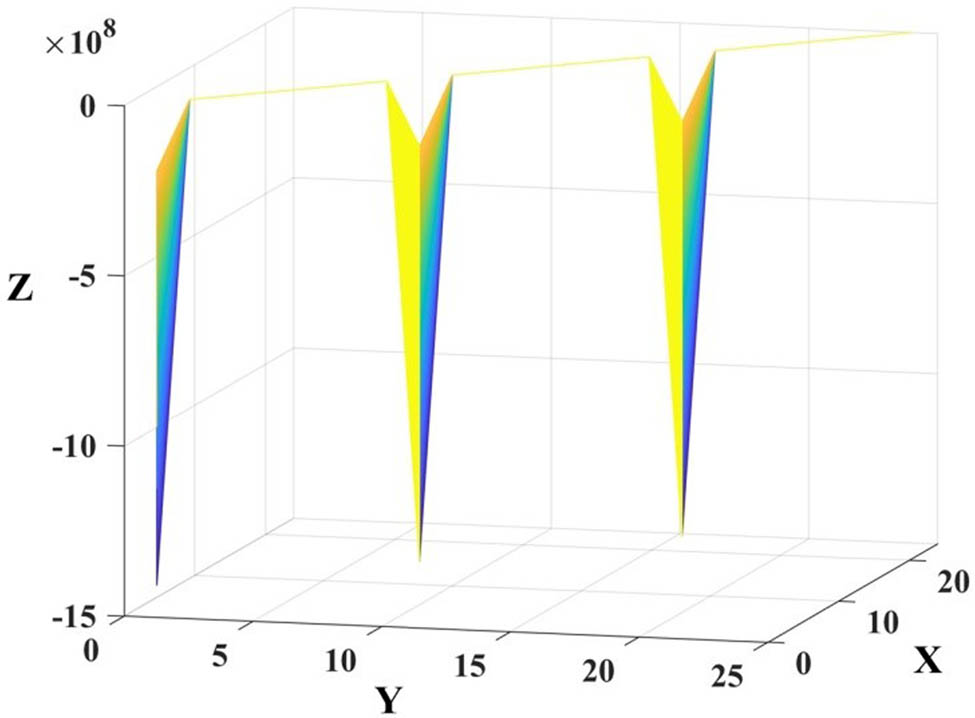
Characteristic vector data point distribution map.

It can be seen from the figure that since the energy value of the fault signal in the low-frequency band is far greater than that in other high-frequency bands, the distribution of wavelet entropy data points is extremely irregular, which is not conducive to the later dimension reduction processing. Therefore, we need to normalize the data. The expression of normalization processing is generally as follows:

(13) y = x − x min x max − x min .

Normalization processing is carried out for the same wavelet entropy column of different fault types. Due to a large amount of data, the normalized feature vector of phase A is still displayed with the initial voltage of 310 V as an example, as shown in Table 2.

Table 2

A-phase normalized eigenvector

Components	S _a(3.0)	S _a(3.1)	S _a(3.2)	…	S _a(3.5)	S _a(3.6)	S _a(3.7)
Normal	0.4749	0.6051	0.6694	…	0.6832	0.6391	0.2060
M1	0.3947	0.4116	0.4703	…	0.3534	0.2783	0.1632
M2	0.5995	0.3323	0.6644	…	0.5445	0.0721	0.6484
M3	0.1988	0.3130	0.1033	…	0.1910	0.9175	0.43636
M4	0.4897	0.1491	0.9649	…	0.4031	0.3814	0.4848
M5	0.9332	0.8798	0.2683	…	0.9563	0.8041	0.6121
M6	0.6737	0.9375	0.0901	…	0.2774	0.4226	0.1939
M1M2	0.6262	0.7381	0.8983	…	0.0502	0.3092	0.2121
M1M3	0.8785	0.7889	0.0409	…	0.8560	0.0526	0.5818
M1M4	0.8934	0.2416	0.6222	…	0.0078	0.3917	0.9852
M1M5	0.9575	0.3329	0.9509	…	0.7643	0.4948	0.1939
M1M6	0.8845	0.2340	0.0619	…	0.2225	0.4020	0.5454
M2M3	0.8637	0.3147	0.9876	…	0.6413	0.7938	0.6181
M2M4	0.8756	0.5499	0.9971	…	0.8324	0.4639	0.9757
M2M5	0.8934	0.9531	0.4234	…	0.6308	0.6701	0.9151
M2M6	0.1766	0.9081	0.5148	…	0.0445	0.3298	0.6235
M3M4	0.9961	0.1599	0.3648	…	0.1073	0.2371	0.2242
M3M5	0.9934	0.9322	0.5351	…	0.6727	0.6804	0.2787
M3M6	0.9967	0.1329	0.0371	…	0.0078	0.9862	0.5696
M4M5	0.9987	0.5688	0.7358	…	0.0602	0.4226	0.2242
M4M6	0.2641	0.4597	0.3296	…	0.4816	0.9587	0.5212
M5M6	0.9878	0.7212	0.4091	…	0.2329	0.5051	0.2606

After normalizing the wavelet entropy eigenvector matrix T, 2,200 × 24 normalized eigenvector T′ is obtained as follows:

(14) T ′ = E 1 , 1 ′ … E 1 , 24 ′ ⋮ ⋱ ⋮ E 2200 , 1 ′ ⋯ E 2200 , 24 ′ .

The distribution of eigenvector data points is shown in Figure 11.

Use the DBSCAN algorithm to screen the landmarks. Use the characteristics that the core point in the DBSCAN clustering algorithm is similar to the landmark definition in the L-ISOMAP method to calculate and filter the landmark; after calculation and adjustment, set the parameters Eps to 1.35 and MinPts to 1; and perform the DBSCAN clustering operation on the feature vector dataset T′, as shown in Figure 12.

Figure 11

Distribution of feature vector T′ data points.

Figure 12

Diagram of DBSCAN clustering operation.

After the DBSCAN clustering operation, the wavelet entropy eigenvector dataset is divided into 101 clusters, i.e., 101 core points are calculated and filtered, and the core point set is set as Ω , i.e., Ω = { E i } ( i = 1 , 2 , ⋯ , 101 ) .

The improved L-ISOMAP method is used to reduce the dimension. The core point set obtained by the DBSCAN clustering algorithm is taken as the landmark set of the L-ISOMAP method, which can effectively avoid the distortion of dimension reduction results caused by the random selection of landmarks by the traditional L-ISOMAP method. PCA method, ISOMAP method, L-ISOMAP method, and DBSCAN-L-ISOMAP method are, respectively, used to reduce the dimension of normalized wavelet entropy feature vector matrix T′. The dimension reduction results are shown in Figure 13.

Figure 13

(a) Result of PCA; (b) result of ISOMAP; (c) result of L-ISOMAP; (d) result of DBSCAN-L-ISOMAP.

The dimension reduction result is consistent with the conclusion in Section 2.2. The dimension reduction data obtained by the DBSCAN-L-ISOMAP method is more evenly distributed, and finally, 2,200 × 2 eigenvector matrix D after dimension reduction is obtained as follows:

(15) D = a 1 , 1 a 1 , 2 a 2 , 1 a 2 , 2 ⋮ ⋮ a 2021 , 1 a 2021 , 2 a 2022 , 1 a 2022 , 2 .

However, the specific dimension reduction effect evaluation also needs to bring the dimension reduction results obtained by different dimension reduction methods into the classifier for fault diagnosis and verify the advantages of the method by comparing the speed and accuracy of fault diagnosis.

4.3 Fault diagnosis analysis

To verify the superiority of the DBSCAN-L-ISOMAP method compared to traditional dimensionality reduction methods, this article uses the SVM as the classifier to classify the fault feature vectors of three-phase VIENNA rectifier wavelet entropy after dimensionality reduction by PCA method, ISOMAP method, L-ISOMAP method, and DBSCAN-L-ISOMAP method in Section 3.2 and compares the dimensionality reduction diagnosis speed and the accuracy of fault recognition.

The SVM is a kind of generalized linear classifier that classifies data in a binary way according to supervised learning. It can also classify data in a nonlinear way through the kernel method. It has the characteristics of strong universality, high robustness, and relatively perfect theory [24].

Identify the six single transistor disconnection fault states and normal states of the three-phase VIENNA rectifier circuit separately. As mentioned above, each fault type has 100 groups of data samples, a total of 700 groups of samples. Using the SVM toolbox in MATLAB, allocate training samples and test samples according to the proportion of 8:2, so the training samples and test samples are 560 groups and 140 groups, respectively. Input the dimension reduction results obtained by different dimension reduction methods in Section 3.2 into the SVM toolbox.

Taking the DBSCAN-L-ISOMAP method as an example, 2,200 × 2 eigenvector matrix D is obtained after dimension reduction. The eigenvector matrix D′ is composed of 700 groups of samples in normal state and single pipe fracture, namely:

(16) D ′ = a 1 , 1 a 1 , 2 a 2 , 1 a 2 , 2 ⋮ ⋮ a 699 , 1 a 699 , 2 a 700 , 1 a 700 , 2 .

Input the eigenvector matrix D′ into the SVM toolbox in MATLAB. After the dimensionality reduction results obtained by the four dimensionality reduction methods are classified by fault identification of the SVM, their diagnosis results are expressed by a confusion matrix. To avoid randomness and ensure high accuracy, each method is tested ten times, and then the classification accuracy and dimensionality reduction diagnosis time are averaged. Figure 14 shows one group of representative diagnosis results.

Figure 14

(a) Result of PCA; (b) result of ISOMAP; (c) result of L-ISOMAP; (d) result of DBSCAN-L-ISOMAP.

The average classification accuracy and average dimensionality reduction diagnostic time obtained by four dimensionality reduction methods using SVMs are shown in Table 3.

Table 3

The average classification accuracy and average dimensionality reduction diagnostic time of different dimensionality reduction methods

Dimension reduction method	Classification accuracy (%)	Dimension reduction diagnosis time (s)
PCA	91.53	1.8
ISOMAP	96.51	13.5
L-ISOMAP	95.12	2.9
DBSCAN-L-ISOMAP	99.08	3.5

It can be seen from Table 3 that the PCA method belongs to the linear dimension reduction method, and the dimension reduction diagnosis speed is the fastest. However, because the fault signals of electronic circuits are nonlinear, the classification accuracy is low; ISOMAP needs to calculate the geodesic distance matrix between two pairs of all data points. Although the classification accuracy is high, its high computational complexity leads to the longest running time. The L-ISOMAP method overcomes the problem of the high computational complexity of the ISOMAP method by selecting landmark points to calculate the geodetic distance matrix between landmark points and other data, which greatly reduces the time for dimension reduction diagnosis. However, due to the randomness of landmark point selection, its classification accuracy is not high. The DBSCAN-L-ISOMAP method uses the DBSCAN clustering algorithm to determine the core points from the data density and filters the landmark points according to the similarity between the core points and the landmark definitions in the L-ISOMAP method, which greatly improves the scientificity of landmark point selection. Although the dimension reduction time is slightly increased due to the addition of the DBSCAN clustering algorithm, the accuracy of fault classification is greatly improved, which verifies the superiority of the DBSCAN-L-ISOMAP method.

We further validated the advantages of the DBSCAN-L-ISOMAP method by comparing and analyzing it with other classic algorithms in manifold learning. The data samples were dimensionally reduced using the Laplace feature mapping Laplacian eigenmaps (LE) method, LLE method, t-distributed stochastic neighbor embedding (t-SNE) method, and DBSCAN-L-ISOMAP method, respectively. The obtained dimensionality reduction results were then used for fault recognition and classification using SVMs. Each method was tested ten times, and then the classification accuracy and dimensionality reduction diagnostic time were averaged. Figure 15 shows one representative set of diagnostic results.

Figure 15

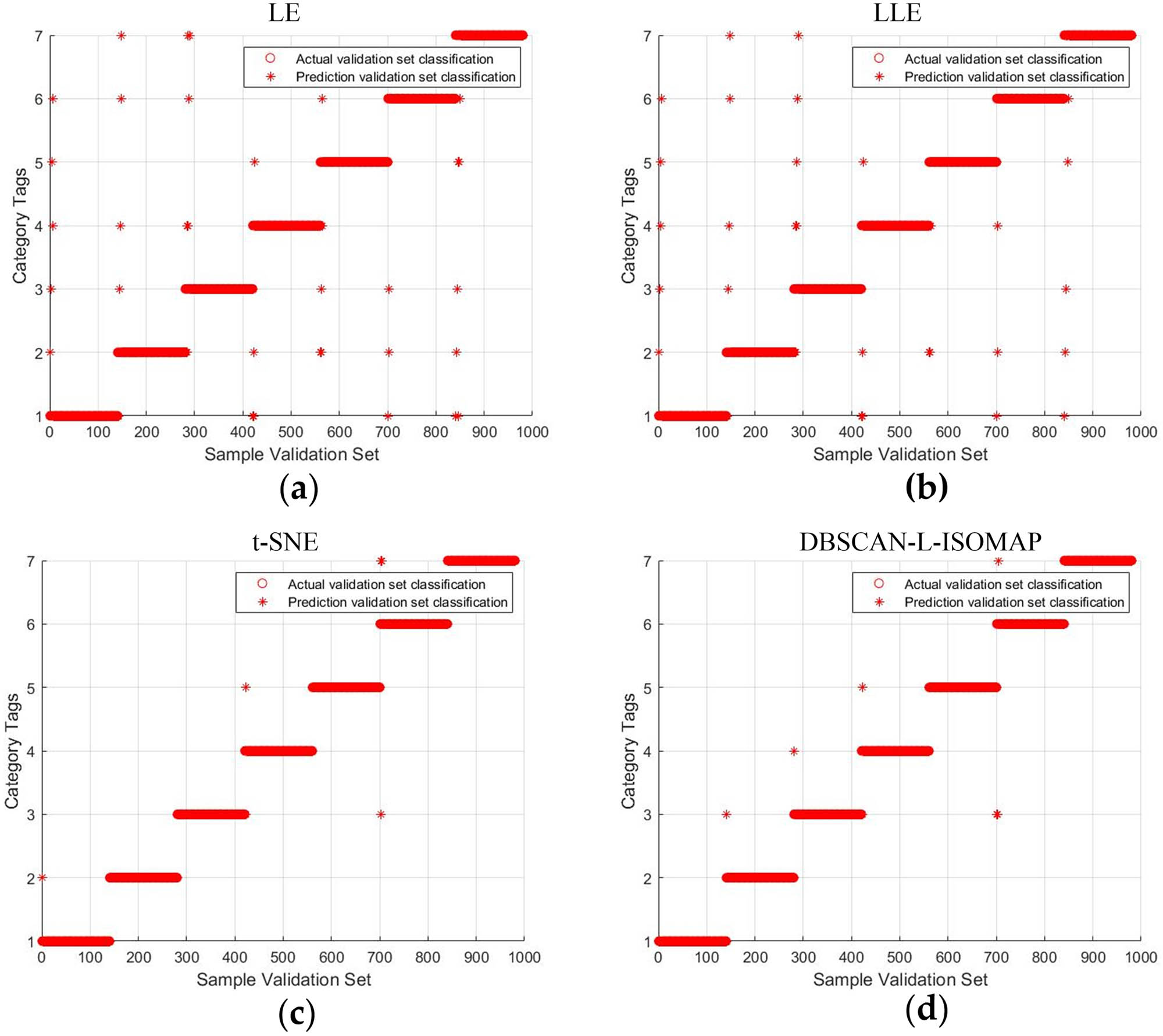
(a) Result of LE; (b) result of LLE; (c) result of t-SNE; (d) result of DBSCAN-L-ISOMAP.

The average classification accuracy and average dimensionality reduction diagnostic time obtained by four dimensionality reduction methods using SVMs are shown in Table 4.

Table 4

The average classification accuracy and average dimensionality reduction diagnostic time of different dimensionality reduction methods

Dimension reduction method	Classification accuracy (%)	Dimension reduction diagnosis time (s)
LE	95.10	2.8
LLE	95.51	3.1
t-SNE	99.29	40.6
DBSCAN-L-ISOMAP	99.08	3.4

It can be seen from Table 4 that because the LE and LLE methods have similar ideas, both belong to local algorithms. The dimensionality reduction of high-dimensional feature vectors is achieved by obtaining the correspondence between high-dimensional space and low-dimensional structure in the local sense, which makes them only need to establish a sparse matrix for calculation, reducing the dimensionality reduction diagnosis time, but it is also easy to have data global structure variations so that the data cannot effectively and correctly reflect the true mapping relationship, causing low classification accuracy for both. The t-SNE method defines similar distributions for points in low-dimensional embeddings by creating probability distributions of high-dimensional samples in a reduced feature space and minimizes the distance between the two distributions in high- and low-dimensional spaces. Therefore, the t-SNE method itself has a certain degree of data aggregation ability, which makes its classification accuracy very high. However, its drawbacks are also very obvious. Due to the large computational complexity, the dimensionality reduction diagnosis time is very long. After considering the balance between classification accuracy and dimensionality reduction diagnosis time, the best dimensionality reduction method is still the DBSCAN-L-ISOMAP method, further verifying the superiority of the DBSCAN-L-ISOMAP method.

5 Conclusions

In this article, we propose an improved marker equidistant feature mapping method based on wavelet packet analysis and the DBSCAN algorithm to solve the problem of feature extraction of electronic circuit fault signals. The feature vector matrix based on wavelet entropy is constructed by using wavelet packet analysis to solve the problem of many original fault signal data points and noise interference. The DBSCAN algorithm is used to calculate and filter the core points of the feature vector dataset, and the feature vector dataset is used as the set of landmarks, which solves the randomness problem of the L-ISOMAP dimension reduction method. The SVM is used to compare the classification accuracy and dimension reduction diagnosis time of the dimension reduction results obtained by PCA method, ISOMAP method, L-ISOMAP method, and DBSCAN-L-ISOMAP method, which verifies the superiority of DBSCAN-L-ISOMAP dimension reduction method and provides a certain reference for the problem of feature extraction of electronic circuit fault signals. However, there are still shortcomings in the method proposed in this article. For example, the selection of individual parameters in the DBSCAN-L-ISOMAP method still requires manual setting, and only a single fault of the electronic component open circuit in electronic circuits has been studied. There are still shortcomings in the validation research of diagnostic methods under different fault conditions, such as short circuits and high resistance. Currently, research and improvement are being carried out on these issues.

Funding information: This research was funded by the National Natural Science Foundation of China (71871219) and the National Defense Pre-Research Project (50904020501).
Author contributions: Conceptualization, Y.Z., Z.C., and G.L.; methodology, Y.Z. and G.L.; software, Y.Z.; validation, Y.Z.; formal analysis, Y.Z.; investigation, Y.Z.; resources, Y.Z. and E.D.; data curation, Y.Z.; writing – original draft preparation, Y.Z.; writing – review and editing, Y.Z. and E.D.; visualization, Y.Z. and Z.W.; supervision, Y.Z. and Z.Z.; project administration, Y.Z.; and funding acquisition, Y.Z. All authors have accepted responsibility for the entire content of this manuscript and approved its submission.
Conflict of interest: The authors state no conflict of interest.

References

[1] Fan JS, Yuan W. Review of parametric fault prediction methods for power electronic circuits. Eng Res Express. 2021;3(4):042002.10.1088/2631-8695/ac340bSearch in Google Scholar

[2] Rongjie W, Yiju Z, Meiqian C, Haifeng Z. Fault diagnosis technology based on Wigner–Ville distribution in power electronics circuit. Int J Electron. 2011;98(9):1247–57.10.1080/00207217.2011.589738Search in Google Scholar

[3] Zhang C, He Y, Yuan L, Xiang S. Analog circuit incipient fault diagnosis method using DBN based features extraction. IEEE Access. 2018;6:23053–64.10.1109/ACCESS.2018.2823765Search in Google Scholar

[4] Wang L, Zhou D, Zhang H, Zhang W, Chen J. Application of relative entropy and gradient boosting decision tree to fault prognosis in electronic circuits. Symmetry. 2018;10(10):495.10.3390/sym10100495Search in Google Scholar

[5] He W, He Y, Li B. Generative adversarial networks with comprehensive wavelet feature for fault diagnosis of analog circuits. IEEE Trans Instrum Meas. 2020;69(9):6640–50.10.1109/TIM.2020.2969008Search in Google Scholar

[6] Qin X, Wang P, Liu Y, Guo L, Sheng G, Jiang X. Research on distribution network fault recognition method based on time-frequency characteristics of fault waveforms. IEEE Access. 2017;6:7291–300.10.1109/ACCESS.2017.2728015Search in Google Scholar

[7] Xu-Sheng G, Hong Q, Xiang-Wei M, Chun-Lan W, Jie Z. Research on ELM soft fault diagnosis of analog circuit based on KSLPP feature extraction. IEEE Access. 2019;7:92517–27.10.1109/ACCESS.2019.2923242Search in Google Scholar

[8] Lin Q, Chen S, Lin CM. Parametric fault diagnosis based on fuzzy cerebellar model neural networks. IEEE Trans Ind Electron. 2018;66(10):8104–15.10.1109/TIE.2018.2884195Search in Google Scholar

[9] Zhang C, Zhao S, He Y. An integrated method of the future capacity and RUL prediction for lithium-ion battery pack. IEEE Trans Veh Technol. 2021;71(3):2601–13.10.1109/TVT.2021.3138959Search in Google Scholar

[10] Zhao S, Zhang C, Wang Y. Lithium-ion battery capacity and remaining useful life prediction using board learning system and long short-term memory neural network. J Energy Storage. 2022;52:104901.10.1016/j.est.2022.104901Search in Google Scholar

[11] Sun Q, Wang Y, Jiang Y. A novel fault diagnostic approach for DC-DC converters based on CSA-DBN. IEEE Access. 2017;6:6273–85.10.1109/ACCESS.2017.2786458Search in Google Scholar

[12] Zhang C, Zhao S, Yang Z, Chen Y. A reliable data-driven state-of-health estimation model for lithium-ion batteries in electric vehicles. Front Energy Res. 2022;10:10.10.3389/fenrg.2022.1013800Search in Google Scholar

[13] Chopra P, Yadav SK. Fault detection and classification by unsupervised feature extraction and dimensionality reduction. Complex & Intell Syst. 2015;1(1):25–33.10.1007/s40747-015-0004-2Search in Google Scholar

[14] Ding S, Li X, Hang J, Wang Y. Application of hybrid dimensionality reduction for fault diagnosis of three-phase inverter in PMSM drive system. Electr Eng. 2019;101(3):813–27.10.1007/s00202-019-00823-8Search in Google Scholar

[15] Kileel J, Moscovich A, Zelesko N, Singer A. Manifold learning with arbitrary norms. J Fourier Anal Appl. 2021;27(5):1–56.10.1007/s00041-021-09879-2Search in Google Scholar

[16] Tenenbaum JB, Silva VD, Langford JC. A global geometric framework for nonlinear dimensionality reduction. Science. 2000;290(5500):2319–23.10.1126/science.290.5500.2319Search in Google Scholar PubMed

[17] Roweis ST, Saul LK. Nonlinear dimensionality reduction by locally linear embedding. Science. 2000;290(5500):2323–6.10.1126/science.290.5500.2323Search in Google Scholar PubMed

[18] Wang Z, Li G, Yao L, Cai Y, Lin T, Zhang J, et al. Intelligent fault detection scheme for constant-speed wind turbines based on improved multiscale fuzzy entropy and adaptive chaotic Aquila optimization-based support vector machine. ISA Trans. 2023;138:582–602.10.1016/j.isatra.2023.03.022Search in Google Scholar PubMed

[19] Millan-Ariño L, Yuan ZF, Oomen ME, Brandenburg S, Chernobrovkin A, Salignon J, et al. An efficient feature extraction approach based on manifold learning for analogue circuits fault diagnosis. Analog Integr Circuits Signal Process. 2020;102:237–52.10.1007/s10470-018-1377-0Search in Google Scholar

[20] Wang Z, Yao L, Cai Y, Zhang J. Mahalanobis semi-supervised mapping and beetle antennae search based support vector machine for wind turbine rolling bearings fault diagnosis. Renew Energy. 2020;155:1312–27.10.1016/j.renene.2020.04.041Search in Google Scholar

[21] Yang B, Xiang M, Zhang Y. Multi-manifold discriminant Isomap for visualization and classification. Pattern Recognit. 2016;55:215–30.10.1016/j.patcog.2016.02.001Search in Google Scholar

[22] Wang Y, Yan Y, Wang Q. Wavelet-based feature extraction in fault diagnosis for biquad high-pass filter circuit. Math Probl Eng. 2016;2016:2016–13.10.1155/2016/5682847Search in Google Scholar

[23] Boonchoo T, Ao X, Liu Y, Zhao W, Zhuang F, He Q. Grid-based DBSCAN: Indexing and inference. Pattern Recognit. 2019;90:271–84.10.1016/j.patcog.2019.01.034Search in Google Scholar

[24] Miao D. Research on fault diagnosis of high-voltage circuit breaker based on support vector machine. Int J Pattern Recognit Artif Intell. 2019;33(6):1959019.10.1142/S0218001419590195Search in Google Scholar

[25] Ahmad K. Wavelet packets and their statistical applications. Singapore: Springer; 2018.10.1007/978-981-13-0268-8Search in Google Scholar

[26] Guan N, Yashiro K, Ohkawa S. On a choice of wavelet bases in the wavelet transform approach. IEEE Trans Antennas Propag. 2000;48(8):1186–91.10.1109/8.884485Search in Google Scholar

[27] Abdelkader R, Chérif BDE, Bendiabdellah A, Kaddour A. Three-phase inverters open-circuit faults diagnosis using an enhanced variational mode decomposition, wavelet packet analysis, and scalar indicators. Electr Eng. 2022;104:1–13.10.1007/s00202-022-01633-1Search in Google Scholar

[28] Gan C, Wu J, Yang S, Hu Y, Cao W. Wavelet packet decomposition-based fault diagnosis scheme for SRM drives with a single current sensor. IEEE Trans Energy Convers. 2015;31(1):303–13.10.1109/TEC.2015.2476835Search in Google Scholar

[29] Chen Y, Zhou L, Pei S, Yu Z, Chen Y, Liu X, et al. KNN-BLOCK DBSCAN: Fast clustering for large-scale data. IEEE Trans Syst Man Cybern Systems. 2019;51(6):3939–53.10.1109/TSMC.2019.2956527Search in Google Scholar

[30] Ienco D, Bordogna G. Fuzzy extensions of the DBScan clustering algorithm. Soft Comput. 2018;22(5):1719–30.10.1007/s00500-016-2435-0Search in Google Scholar

[31] Luchi D, Rodrigues AL, Varejão FM. Sampling approaches for applying DBSCAN to large datasets. Pattern Recognit Lett. 2019;117:90–6.10.1016/j.patrec.2018.12.010Search in Google Scholar

[32] Zhai Y, Wang N, Zhang L, Hao L, Hao C. Automatic crop classification in Northeastern China by improved nonlinear dimensionality reduction for satellite image time series. Remote Sens. 2020;12(17):2726.10.3390/rs12172726Search in Google Scholar

[33] Orsenigo C. An improved set covering problem for Isomap supervised landmark selection. Pattern Recognit Lett. 2014;49:131–7.10.1016/j.patrec.2014.07.007Search in Google Scholar

[34] Shi H, Yin B, Kang Y, Shao C, Gui J. Robust L-Isomap with a novel landmark selection method. Math Probl Eng. 2017;2017:3930957.10.1155/2017/3930957Search in Google Scholar

[35] Li X, Sun Y, Wang H, Su M, Huang S. A hybrid control scheme for three-phase Vienna rectifiers. IEEE Trans Power Electron. 2017;33(1):629–40.10.1109/TPEL.2017.2661382Search in Google Scholar

[36] Wang Y, Li Y, Guo X, Huang S. Hybrid space vector PWM strategy for three-phase VIENNA rectifiers. Sensors. 2022;22(17):6607.10.3390/s22176607Search in Google Scholar PubMed PubMed Central

[37] Zhang L, Zhao R, Ju P, Ji C, Zou Y, Ming Y, et al. A modified DPWM with neutral point voltage balance capability for three-phase Vienna rectifiers. IEEE Trans Power Electron. 2020;36(1):263–73.10.1109/TPEL.2020.3002660Search in Google Scholar

Received: 2022-11-30

Revised: 2023-05-09

Accepted: 2023-05-23

Published Online: 2023-07-12

This work is licensed under the Creative Commons Attribution 4.0 International License.

Articles in the same Issue

https://doi.org/10.1515/phys-2022-0254

Keywords for this article

electronic circuit failure; feature extraction; wavelet packet analysis; DBSCAN algorithm; isometric feature mapping method of landmarks; support vector machines

Creative Commons

BY 4.0