Different lump k-soliton solutions to (2+1)-dimensional KdV system using Hirota binary Bell polynomials

Xingxing Wu; Jalil Manafian; Gurpreet Singh; Baharak Eslami; Abdullah Aldurayhim; Noor Alhuda Mohammad Ali khalil; Ahmed Alawadi

doi:10.1515/phys-2023-0167

Article Open Access

Different lump k-soliton solutions to (2+1)-dimensional KdV system using Hirota binary Bell polynomials

Xingxing Wu , Jalil Manafian , Gurpreet Singh , Baharak Eslami , Abdullah Aldurayhim , Noor Alhuda Mohammad Ali khalil and Ahmed Alawadi

Published/Copyright: December 31, 2023

Published by

Become an author with De Gruyter Brill

Submit Manuscript Author Information Explore this Subject

From the journal Open Physics Volume 21 Issue 1

Abstract

In this article, the (2+1)-dimensional KdV equation by Hirota’s bilinear scheme is studied. Besides, the binary bell polynomials and then the bilinear form is created. In addition, an interaction lump with k -soliton solutions of the addressed system with known coefficients is presented. With the assistance of the stated methodology, a cloaked form of an analytical solution is discovered in expressions of lump-soliton rational functions with a few lovable parameters. Solutions to this study’s problems are identified specifically as belonging to the lump-one, two, three, and four soliton solutions. By defining the specific advantages of the epitomized parameters by the depiction of figures and by interpreting the physical occurrences are established acceptable soliton arrangements and dealt with the physical importance of the obtained arrangements. Finally, under certain conditions, the physical behavior of solutions is analyzed by using the mentioned method. Moreover, the graphs with high resolutions including three-dimensional plots, density plots, and two-dimensional plots to determine a deep understanding of plotted solutions that will arise in the applied mathematics and nonlinear physics are employed.

Keywords: Hirota bilinear scheme; (2+1)-dimensional KdV equation; interaction lump with k-soliton solutions

1 Introduction

Nonlinear partial differential equations (NLPDEs) have been used in various domains from physics to engineering, chemistry and biology, and environmental monitoring system as mathematical models of complex physical processes [1–3]. In the investigation of nonlinear physical events, the exact solutions to nonlinear evolution equations (NLEEs) play a significant role. To obtain the exact solutions of the NLEEs, the Cole–Hopf transformation is also widely used, e.g., on the miscellaneous soliton waves in metamaterials model [4], diffusive susceptible-infected-susceptible epidemic model [5], and the nonlinear vibration and dispersive wave systems [6]. The optical soliton solutions to the Kudryashov’s quintuple self-phase modulation with dual-form [7], the unified method [8], homogeneous Neumann boundary conditions [9], the Hirota bilinear method [10–12], the acid–base theory of surfaces [13], the deep learning algorithm [14], distributed parallel particle swarm optimization [15], image processing and flow field reconstruction algorithm [16], behaviors in group decision-making systems [17], sector beam synthesis in linear antenna arrays [18], a hybrid stochastic-deterministic approach [19], a novel fractional-order multiple-model type-3 [20], N -lump and interaction solutions [21], derivation of optimized equations for estimation of dispersion coefficient [22], truss optimization with metaheuristic algorithms and under dynamic loading [23], an improved Hirota bilinear method [24], optimal bidding and offering strategies [25], quantum chromo dynamics sum rules [26,27], a hybrid convolutional neural network [28], the proton-exchange membrane fuel cells based on deep learning [29], the robust optimization technique [30,31], the network governance step by step method [32], and the neural network method [33] are just few of the methodologies discovered for obtaining explicit solutions to NLEEs. Solitary wave solutions, periodic wave solutions, shock wave solutions, and other exact solutions were achieved using these methods. The interested reader can see some good topics in previous studies [34]–[40].

The objective of this research is to go further into the subject of how to find solitary waves and lump solutions to the (2+1)-dimensional Korteweg–de Vries (KdV) equation. To achieve this, we have adopted the Hirota bilinear method and the binary bell-polynomials (BBPs) approach.

Ma [41] invented the lump transformation as a straightforward and easy approach for obtaining solutions as a combination of positive functions to NLPDEs. Zhao et al. [42] obtained the interaction between lump and two kink, periodic, wave, and other solutions for the Burger system by using the multidimensional Bell polynomials and based on the binary Bäcklund transformations and the generalized Bell polynomials. Akter and Hafez [43] explored the head-on collision between two-counter propagating positron acoustic solitons and double layers in an unmagnetized collisionless plasma. By using a technique of the symbolic computations utilizing Maple, Ma obtained the lump-soliton, lump-kink, and lump-periodic solutions, which were computed for the Hirota–Satsuma–Ito equation in (2+1) dimensions [44]. The same author explored the novel (2+1)-dimensional nonlinear equations containing lump solutions via the Hirota bilinear method and he formulated a combined fourth-order nonlinear equation for guaranteeing the existence of lump solutions [45]. N-soliton solutions and dynamic property analysis of the generalized three-component Hirota–Satsuma coupled KdV equation [46] and a (2+1)-dimensional combined equation [47] were investigated by capable scholarships. Numerous exact and lump soliton solutions have been achieved using the logarithm transformation.

The Hirota BBPs unifies the Hirota bilinear method and the BBPs to give systematic and straightforward handling of the solution process of nonlinear equations. We have employed an improved version of the Hirota BBPs approach to acquire variety lump solutions to the (2+1)-dimensional KdV system. Lump solutions construct positive quadratic function solutions of a novel type, and also lump-multi-soliton combines a positive quadratic function and different exponential functions solutions. So it is feasible to develop lump and lump-solitons solutions to NLPDEs with simplifying the complicated computations. For this purpose, the Hirota bilinear form along with BBPs of the proposed problem is utilized to create the mentioned solutions.

The following (2+1)-dimensional Hietarinta equation has been introduced and studied by some researchers, for example, the spectral transform of a KdV equation in two space dimensions by using of the weak Lax pair [48], single- and multi-solitary wave solutions [49], generalized dromion solutions of the (2+1)-dimensional KdV equation [50], the localized excitations of the (2+1)-dimensional KdV equation [51], and solitons and singular solitons for the Gardner-KP equation [52]. The (2+1)-dimensional KdV equation [53] is considered as follows:

(1.1) u t + 3 ( u v ) x − u x x x = 0 , u x = v y ,

or u = ∫ x v y d x , where u = u ( x , y , t ) and v = v ( x , y , t ) . Wang et al. [53] offered the periodic type of three-wave solutions for Eq. (1.1) using Hirota’s bilinear form. Based on the Painlevé analysis in the study by Wang et al. [53], the new exact periodic cross-kink wave solutions for the (2+1)-dimensional KdV equation were obtained by Liu and Ye [54]. The following transformations are obtained

(1.2) u ( x , y , t ) = u 0 + 2 [ ϕ ( x , y , t ) ] x y , v ( x , y , t ) = v 0 + 2 [ ϕ ( x , y , t ) ] x x ,

where here u 0 and v 0 are two constants and ϕ ( x , y , t ) is uncertain function. According to the Painlevé analysis, the bilinear formalism of the (2+1)-dimensional KdV equation was obtained in the study by Liu et al. [55]. In the study by Liu et al. [56], the interaction between lump-type solutions to (2+1)-dimensional asymmetrical Nizhnik–Novikov–Veselov equation were obtained. Ilhan et al. [57] used the Hirota bilinear method for investigating the third-order evolution equation to determine the soliton-type solutions.

The BBPs was considered in the study by Shen et al. [58]. Based on the study by Li et al. [24], ℘ = ℘ ( x 1 , x 2 , … , x n ) be a C ∞ function with the following multi-variables:

(1.3) ϒ n 1 x 1 , … , n j x j ( ℘ ) ≡ ϒ n 1 , … , n j ( ℘ b 1 x 1 , … , b j x j ) = e − ℘ ∂ x 1 n 1 … ∂ x j n j e ℘ ,

with the below formalism (BBPs [24])

℘ b 1 x 1 , … , b j x j = ∂ x 1 b 1 … ∂ x j b j ℘ , ℘ 0 x i ≡ ℘ , b 1 = 0 , … , n 1 ; … ; b j = 0 , … , n j ,

one become

ϒ 1 ( ℘ ) = ℘ x , ϒ 2 ( ℘ ) = ℘ 2 x + ℘ x 2 , ϒ 3 ( ℘ ) = ℘ 3 x + 3 ℘ x ℘ 2 x + ℘ x 3 , … , ℘ = ℘ ( x , t ) ,

(1.4) ϒ x , t ( ℘ ) = ℘ x , t + ℘ x ℘ t , ϒ 2 x , t ( ℘ ) = ℘ 2 x , t + ℘ 2 x ℘ t + 2 ℘ x , t ℘ x + ℘ x 2 ℘ t , … .

The multidimensional BBPs can be written as follows:

(1.5) Σ n 1 x 1 , … , n j x j ( μ 1 , μ 2 ) = ϒ n 1 , … , n j ( ℘ ) ∣ ℘ b 1 x 1 , … , b j x j = μ 1 b 1 x 1 , … , b j x j , b 1 + b 2 + … + b j , is odd μ 2 b 1 x 1 , … , b j x j , b 1 + b 2 + … + b j , is even.

We can find the required relations as the following:

(1.6) Σ x ( μ 1 ) = μ 1 x , Σ 2 x ( μ 1 , μ 2 ) = μ 2 2 x + μ 1 x 2 , Σ x , t ( μ 1 , μ 2 ) = μ 2 x , t + μ 1 x μ 1 t , … .

Proposition 1.1

Let μ 1 = ln ( Ω 1 ∕ Ω 2 ) and μ 2 = ln ( Ω 1 Ω 2 ) , and hence, the relation between BBPs and Hirota D-operator shows

(1.7) Σ n 1 x 1 , … , n j x j ( μ 1 , μ 2 ) ∣ μ 1 = ln ( Ω 1 ∕ Ω 2 ) , μ 2 = ln ( Ω 1 Ω 2 ) = ( Ω 1 Ω 2 ) − 1 D x 1 n 1 … D x j n j Ω 1 Ω 2 ,

with the following derivative

(1.8) ∏ i = 1 j D x i n i g ⋅ η = ∏ i = 1 j ∂ ∂ x i − ∂ ∂ x i ′ n i Ω 1 ( x 1 , … , x j ) Ω 2 ( x 1 ′ , … , x j ′ ) x 1 = x 1 ′ , … , x j = x j ′ .

Proposition 1.2

Take Ξ ( γ ) = ∑ i δ i P d 1 x 1 , … , d j x j = 0 and μ 1 = ln ( Ω 1 ∕ Ω 2 ) , μ 1 = ln ( Ω 1 Ω 2 ) , we consider

(1.9) ∑ i δ 1 i ϒ n 1 x 1 , … , n j x j ( μ 1 , μ 2 ) = 0 , ∑ i δ 1 i ϒ d 1 x 1 , … , d j x j ( μ 1 , μ 2 ) = 0 ,

with the following mentioned conditions:

(1.10) S ( γ ′ , γ ) = S ( γ ′ ) − S ( γ ) = S ( μ 2 + μ 1 ) − S ( μ 2 − μ 1 ) = 0 .

The generalized Bell polynomials ϒ n 1 x 1 , … , n j x j ( ξ ) is presented as follows:

(1.11) ( Ω 1 Ω 2 ) − 1 D x 1 n 1 … D x j n j Ω 1 Ω 2 = Σ n 1 x 1 , … , n j x j ( μ 1 , μ 2 ) ∣ μ 1 = ln ( Ω 1 ∕ Ω 2 ) , μ 2 = ln ( Ω 1 Ω 2 ) = Σ n 1 x 1 , … , n j x j ( μ 1 , μ 1 + γ ) ∣ μ 1 = ln ( Ω 1 ∕ Ω 2 ) , γ = ln ( Ω 1 Ω 2 ) = ∑ k 1 n 1 … ∑ k j n j ∏ i = 1 j n i k i P k 1 x 1 , … , k j x j ( γ ) ϒ ( n 1 − k 1 ) x 1 , … , ( n j − k j ) x j ( μ 1 ) .

The Cole–Hopf relation is given as follows:

(1.12) ϒ k 1 x 1 , … , k j x j ( μ 1 = ln ( τ ) ) = τ n 1 x 1 , … , n j x j τ ,

(1.13) ( Ω 1 Ω 2 ) − 1 D x 1 n 1 … D x j n j Ω 1 Ω 2 ∣ Ω 2 = exp ( γ ∕ 2 ) , Ω 1 ∕ Ω 2 = τ = τ − 1 ∑ k 1 n 1 … ∑ k j n j ∏ l = 1 j n l k l P k 1 x 1 , … , k l x l ( γ ) τ ( n 1 − k 1 ) x 1 , … , ( n d − k l ) x l ,

with

(1.14) ϒ t ( μ 1 ) = τ t τ , ϒ 2 x ( μ 1 , β ) = γ 2 x + τ 2 x τ , ϒ 2 x , y ( μ 1 , μ 2 ) = γ 2 x τ y τ + 2 γ x , y τ x τ + τ 2 x , y τ .

To be used in later stages, the mentioned issue with the bilinear form to the (2+1)-dimensional KdV equation is obtained from

(1.15) ( D G ) ( ϕ . ϕ ) = ∏ i = 1 3 ∂ ∂ x i − ∂ ∂ x i ′ n i Θ ( x 1 , x 2 , x 3 ) Δ ( x 1 ′ , x 2 ′ , x 3 ′ ) x 1 = x 1 ′ , x 2 = x 2 ′ , x 3 = x 3 ′ = 2 [ ( ϕ ϕ y t − ϕ y ϕ t ) + ( ϕ ϕ x x x y − 3 ϕ x ϕ x x y + 3 ϕ x x ϕ x y − ϕ x x x ϕ y ) + 3 u 0 ( ϕ ϕ x x − ϕ x 2 ) + 3 v 0 ( ϕ ϕ x y − ϕ x ϕ y ) ] = [ D y D t + D y D x 3 + 3 u 0 D x 2 + 3 v 0 D x D y ] ϕ . ϕ = 0 .

Gang et al. [59] studied an integrable of the generalized Calogero–Bogoyavlenskii–Schiff–Bogoyavlensky–Konopelchenko equation by employing Hirota’s bilinear method and obtained the multiple-soliton solutions. Zhao et al. [60] investigated the N-soliton solutions of a generalized (2+1)-dimensional Hirota–Satsuma–Ito equation by means of the bilinear method and three kinds of high-order hybrid solutions were presented. Based on the bilinear method for a generalized (2+1)-dimensional nonlinear wave equation, the N-soliton solutions, were obtained in the study by He et al. [61]. In the study of lump-N soliton solutions, Tan et al. investigated M-solitons for the (2+1)-dimensional KdV system [62,63] and some new lump solutions of the (2+1)-dimensional breaking Soliton system [64] by the help of Hirota bilinear technique. The Hirota bilinear scheme and τ -function formalism were used in the study of localized nonlinear wave interaction structures generated by the six-soliton solutions of the generalized Kadomtsev–Petviashvili equation [65]. Cheng et al. [66] investigated an extended KdV equation in (2+1)-dimensions, which cannot be directly bilinearized.

Based on the invariant subspace method, the Lie symmetries including Riemann–Liouville and Erdelyi–Kober fractional derivatives of time-fractional form of the Gardner equation have been studied [67]. Numerical analysis of bioconvective heat and mass transfer across a nonlinear stretching sheet with hybrid nanofluids was investigated in the study by [68]. The (2+1)-dimensional Benjamin–Bona–Mahony–Burgers model was considered and reduced to the bilinear form by using the Hirota bilinear scheme [69]. The modified Oskolkov equation in incompressible viscoelastic Kelvin–Voigt fluid and fluid dynamics was considered using the modified simple equation method to retrieve various dynamical structural solutions of the nonlinear models [70].

Some closed-form invariant solutions and dynamical behavior of multiple solitons for the (2+1)-dimensional nonlinear r th dispersionless Dym equation using the Lie symmetry approach have been found by Kumar et al. [71]. The (2+1)-dimensional Kadomtsev–Petviashvili–Benjamin–Bona–Mahony equation by using two powerful techniques, the Lie symmetry method and the generalized exponential rational function method, with the help of symbolic computations has been worked [72]. The (2+1)-dimensional modified Calogero–Bogoyavlenskii–Schiff equation using the Lie group of transformation method was studied, and all of the vector fields, commutation table, invariant surface condition, Lie symmetry reductions, infinitesimal generators, and explicit solutions were constructed [73].

The Hirota bilinear method was used to the equation of the shallow water wave in oceanography and atmospheric science was extended to (3+1) dimensions [74]. The (2+1)-dimensional variable-coefficient Caudrey–Dodd–Gibbon–Kotera–Sawada model used in soliton hypothesis and implemented by operating the Hirota bilinear scheme was studied [75]. Zhou et al. [76] studied the (3+1)-dimensional variable-coefficient nonlinear wave equation, which is taken in soliton theory and generated by utilizing the Hirota bilinear technique and obtained some new exact analytical solutions, containing interaction between a lump-two kink solitons and interaction between two lumps.

The important topic of this article is to gain the valuable results on exact analytical solutions, containing interaction lump with k -soliton solutions for the (2+1)-dimensional KdV equation. There is a famous fact that soliton equations can be rewritten as the Hirota bilinear forms by applying the Hirota bilinear derivatives. These good results are shown that the Hirota bilinear derivative is a powerful mathematical tool to handle nonlinear integrable equation from nature. On the basis of the Hirota bilinear forms of this considered equation, a class of good results such as the lump-1 soliton solutions, lump double soliton solutions, N-soliton solutions, and rational solutions was obtained.

The arrangement and organization of this article is given as follows. In Section 2, the interaction lump with k -soliton solutions in subsections including lump-one, two, three, and four soliton solutions to the (2+1)-D KdV equation by employing the BBP and the bilinear form of Eq. (1.15) and according to Hirota’s direct scheme are discussed. Finally, conclusions are given is Section 3.

2 Resonant soliton solutions

The lump-one, two, three, and four soliton wave solutions are studied and presented in the following subsections. The general form of the lump with k -soliton solution can be written as follows:

(2.1) ϕ = a 1 2 + a 2 2 + ∑ l = 1 k λ l exp ( a l + 2 ) + λ k + 1 ,

where

a l = λ l x + λ l + 1 y + λ l + 2 t + λ l + 3 , l = 1 , 2 , … , k .

2.1 Lump-1 soliton solutions

There are many aforementioned equations, and we have to specify the number of equation as follows:

(2.2) ϕ = a 1 2 + a 2 2 + λ 13 exp ( a 3 ) + λ 14 , a 1 = λ 3 t + λ 1 x + λ 2 y + λ 4 , a 2 = λ 7 t + λ 5 x + λ 6 y + λ 8 , a 3 = λ 11 t + λ 9 x + λ 10 y + λ 12 .

Afterward, the values λ l , ( l = 1 : 14 ) will be received. By substituting Eq. (2.2) into (1.15) and taking the coefficients of exponential function e Φ ( x , y , t ) and polynomials function with regard to x , y , t to zero, we yield a system of nonlinear algebraic for constants λ l , ( l = 1 : 14 ) . We can obtain the relationship between u = u 0 + 2 ( ln ϕ ) x y and v = v 0 + 2 ( ln ϕ ) x x by using of the logarithm transformation.

2.1.1 Category I solutions

(2.3) λ 1 = − λ 5 λ 6 λ 2 , λ 2 = λ 2 , λ 3 = 3 λ 5 λ 6 v 0 λ 2 , λ 4 = λ 4 , λ 5 = λ 5 , λ 6 = λ 6 , λ 7 = − 3 λ 5 v 0 , λ 8 = λ 8 , λ 9 = λ 9 , λ 10 = 0 , λ 11 = − λ 9 3 − 3 λ 9 v 0 , λ 12 = λ 12 , λ 13 = λ 13 , λ 14 = λ 14 ,

where λ s are free values for s = 2 , 4 , 5 , 6 , 8 , 9 , 12 , 13 , 14 . To obtain the real function, we need the following condition:

(2.4) λ 2 ≠ 0 .

Along with the bilinear equation and using the values of parameters obtained in Eq. (2.3) in Eq. (2.2), we acquire

(2.5) u 1 = u 0 + 2 ( ln ϕ ( x , y , t ) ) x y = u 0 + 2 ∂ 2 ∂ y ∂ x ϕ ( x , y , t ) ϕ ( x , y , t ) − ∂ ∂ x ϕ ( x , y , t ) ∂ ∂ y ϕ ( x , y , t ) ( ϕ ( x , y , t ) ) 2 ,

v 1 = v 0 + 2 ( ln ϕ ( x , y , t ) ) x x = v 0 + 2 ∂ 2 ∂ x 2 ϕ ( x , y , t ) ϕ ( x , y , t ) − ∂ ∂ x ϕ ( x , y , t ) 2 ( ϕ ( x , y , t ) ) 2 ,

ϕ = 3 λ 5 λ 6 v 0 t λ 2 − x λ 5 λ 6 λ 2 + λ 2 y + λ 4 2 + ( − 3 t λ 5 v 0 + x λ 5 + y λ 6 + λ 8 ) 2 + λ 13 e ( − λ 9 3 − 3 λ 9 v 0 ) t + λ 9 x + λ 12 + λ 14 .

If x → ∞ , then lump-one soliton solution of solution functions u and v with any time. Figures 1 and 2 show the dynamical properties of lump and move forward of soliton as exponential function with plots of u and v by the following determined values:

λ 2 = 2 , λ 4 = 2 , λ 5 = 1 , λ 6 = 1 , λ 8 = 1 , λ 9 = 1 , λ 12 = 1 , λ 13 = 1 , λ 14 = 1 , v 0 = 2 , t = − 1 ,

u 1 = − 160 ( 30 + 5 x + 2 e 8 + x ) ( 1 + y ) ( 5 x 2 + 20 y 2 + 4 e 8 + x + 60 x + 40 y + 204 ) 2 ,

v 1 = 2 ( 5 x 2 + 20 y 2 + 4 e 8 + x + 60 x + 40 y + 204 ) 2 × [ 25 x 4 + 200 x 2 y 2 + 400 y 4 + 60 e 8 + x x 2 + 240 e 8 + x y 2 + 600 x 3 + 400 x 2 y + 2,400 x y 2 + 1,600 y 3 + 16 ( e 8 + x ) 2 + 640 x e 8 + x + 480 e 8 + x y + 5,590 x 2 + 4,800 x y + 9,960 y 2 + 2,008 e 8 + x + 23,880 x + 16,720 y + 40,056 ]

in Eq. (2.5). By using the aforementioned parameters, the structural properties among a lump and one parallel y -kink of solutions are shown in Figures 1 and 2 and with illustrations of 3D and 2D plots. It is remarkable that changing the parameters affects the final results.

$Figure 1 Plot of lump-one soliton solution (2.5) ( u 1 {u}_{1} ) (3D, density, and 2D plot y y ).$

Figure 1

Plot of lump-one soliton solution (2.5) ( u 1 ) (3D, density, and 2D plot y ).

$Figure 2 Plot of lump-one soliton solution (2.5) ( v 1 {v}_{1} ) (3D, density, and 2D plot y y ).$

Figure 2

Plot of lump-one soliton solution (2.5) ( v 1 ) (3D, density, and 2D plot y ).

2.1.2 Set II solutions

(2.6) λ 1 = λ 2 = λ 3 = 0 , λ 4 = λ 4 , λ 5 = λ 7 = 0 , λ 6 = λ 6 , λ 7 = 0 , λ 8 = λ 8 , λ 9 = λ 9 , λ 10 = λ 10 , λ 11 = − λ 9 3 − 3 λ 9 v 0 , λ 12 = λ 12 , λ 13 = λ 13 , λ 14 = λ 14 ,

where λ s are free values for s = 4 , 6 , 8 , 9 , 10 , 12 , 13 , 14 . Using the values of parameter obtained in Eq. (2.6) in Eq. (2.2) yields

(2.7) u 2 = u 0 + 2 λ 13 λ 9 λ 10 e ( − λ 9 3 − 3 λ 9 v 0 ) t + λ 9 x + y λ 10 + λ 12 λ 4 2 + ( y λ 6 + λ 8 ) 2 + λ 13 e ( − λ 9 3 − 3 λ 9 v 0 ) t + λ 9 x + y λ 10 + λ 12 + λ 14

− 2 λ 13 λ 9 e ( − λ 9 3 − 3 λ 9 v 0 ) t + λ 9 x + y λ 10 + λ 12 ( 2 ( y λ 6 + λ 8 ) λ 6 + λ 13 λ 10 e ( − λ 9 3 − 3 λ 9 v 0 ) t + λ 9 x + y λ 10 + λ 12 ) ( λ 4 2 + ( y λ 6 + λ 8 ) 2 + λ 13 e ( − λ 9 3 − 3 λ 9 v 0 ) t + λ 9 x + y λ 10 + λ 12 + λ 14 ) 2 ,

v 2 = v 0 + 2 λ 13 λ 9 2 e ( − λ 9 3 − 3 λ 9 v 0 ) t + λ 9 x + y λ 10 + λ 12 λ 4 2 + ( y λ 6 + λ 8 ) 2 + λ 13 e ( − λ 9 3 − 3 λ 9 v 0 ) t + λ 9 x + y λ 10 + λ 12 + λ 14

− 2 λ 13 2 λ 9 2 ( e ( − λ 9 3 − 3 λ 9 v 0 ) t + λ 9 x + y λ 10 + λ 12 ) 2 ( λ 4 2 + ( y λ 6 + λ 8 ) 2 + λ 13 e ( − λ 9 3 − 3 λ 9 v 0 ) t + λ 9 x + y λ 10 + λ 12 + λ 14 ) 2 .

If x → ∞ with λ 13 > 0 , then lump-one soliton solution of solution functions u 2 and v 2 with any time. Figures 3 and Figure 4 show the dynamical properties of lump and move forward of soliton as exponential function by plots of u and v by the below determined values

λ 4 = 2 , λ 6 = 1 , λ 8 = 1 , λ 9 = 1 , λ 10 = 1 , λ 12 = 1 , λ 13 = 1 , λ 14 = 1 , u 0 = 1 , v 0 = 2 , t = 1 ,

u 2 = 2 y 4 + 3 e − 6 + x + y y 2 + 4 y 3 + ( e − 6 + x + y ) 2 + 6 e − 6 + x + y y + 16 y 2 + 18 e − 6 + x + y + 24 y + 36 ( y 2 + e − 6 + x + y + 2 y + 6 ) 2 ,

v 2 = v 0 + 2 λ 13 λ 9 2 e − t λ 9 3 − 3 t λ 9 v 0 + λ 9 x + y λ 10 + λ 12 ( y 2 λ 6 2 + 2 y λ 6 λ 8 + λ 4 2 + λ 8 2 + λ 14 ) ( y 2 λ 6 2 + 2 y λ 6 λ 8 + λ 13 e − t λ 9 3 − 3 t λ 9 v 0 + λ 9 x + y λ 10 + λ 12 + λ 4 2 + λ 8 2 + λ 14 ) 2 ,

in Eq. (2.7). By using of the aforementioned parameters the physical properties among a lump and one parallel y -kink of solutions as shown in Figures 3 and 4 and by 3D, density, and 2D graphs.

$Figure 3 Graph of lump-one soliton solution (2.7) ( u 2 {u}_{2} ) (3D, density, and 2D plot y y ).$

Figure 3

Graph of lump-one soliton solution (2.7) ( u 2 ) (3D, density, and 2D plot y ).

$Figure 4 Graph of lump-one soliton solution (2.7) ( v 2 {v}_{2} ) (3D, density, and 2D plot y y ).$

Figure 4

Graph of lump-one soliton solution (2.7) ( v 2 ) (3D, density, and 2D plot y ).

2.2 Lump-2 soliton solutions

To find the exact forms of solutions of the Eq. (1.15), we define the lump-two soliton solutions as follows:

(2.8) ϕ = a 1 2 + a 2 2 + λ 17 exp ( a 3 ) + λ 18 exp ( a 4 ) + λ 19 exp ( a 3 + a 4 ) + λ 20 ,

a 1 = λ 3 t + λ 1 x + λ 2 y + λ 4 , a 2 = λ 7 t + λ 5 x + λ 6 y + λ 8 ,

a 3 = λ 11 t + λ 9 x + λ 10 y + λ 12 , a 4 = λ 15 t + λ 13 x + λ 14 y + λ 16 .

Afterward, the values λ l , ( l = 1 : 20 ) arbitrary constants that are to be discovered. By inserting Eq. (2.8) into Eq. (1.15), a system of algebraic equations is fulfilled. We acquire the following cases from the solutions of the system:

2.2.1 Set I solutions

(2.9) u 0 = 0 , λ 1 = λ 3 = λ 5 = λ 7 = 0 , λ s = λ s , s = 2 , 4 , 6 , 8 , 12 , 13 , 16 , λ 9 = − λ 13 , λ 10 = − λ 14 , λ 11 = λ 13 ( λ 13 2 + 3 v 0 ) , λ 15 = − λ 13 ( λ 13 2 + 3 v 0 ) ,

where λ s are free values for s = 2 , 4 , 6 , 8 , 12 , 13 , 16 , … , 20 . Along with the bilinear equation and using the values of parameters determined in Eq. (2.9) in Eq. (2.8), we yield

(2.10) u = u 0 + 2 ( ln ϕ ( x , y , t ) ) x y = u 0 + 2 ∂ 2 ∂ y ∂ x ϕ ( x , y , t ) ϕ ( x , y , t ) − ∂ ∂ x ϕ ( x , y , t ) ∂ ∂ y ϕ ( x , y , t ) ( ϕ ( x , y , t ) ) 2 ,

v = v 0 + 2 ( ln ϕ ( x , y , t ) ) x x = v 0 + 2 ∂ 2 ∂ x 2 ϕ ( x , y , t ) ϕ ( x , y , t ) − ∂ ∂ x ϕ ( x , y , t ) 2 ( ϕ ( x , y , t ) ) 2 ,

ϕ = ( y λ 2 + λ 4 ) 2 + ( y λ 6 + λ 8 ) 2 + λ 17 e λ 13 ( λ 13 2 + 3 v 0 ) t − λ 13 x + λ 14 y + λ 12 + λ 18 e − λ 13 ( λ 13 2 + 3 v 0 ) t + λ 13 x + λ 14 y + λ 16 + λ 19 e 2 λ 14 y + λ 12 + λ 16 + λ 20 .

If x → ∞ , then we obtain lump-two soliton solution of solution functions u and v with any time. Figures 5 and 6 show the dynamical properties of lump and move forward of solitons as two exponential functions by plots of u and v by the following determined amounts:

λ 2 = 2 , λ 4 = 1 , λ 6 = λ 8 = λ 12 = λ 14 = λ 16 = λ 17 = 1 , λ 18 = 2 , λ 19 = 3 , λ 20 = 1 , v 0 = 2 , t = 1 ,

u 1 = 2 ( e 8 − x + y − 2 e − 6 + x + y ) ( − 5 y 2 + 3 e 2 y + 2 + 4 y + 3 ) ( 5 y 2 + e 8 − x + y + 2 e − 6 + x + y + 3 e 2 y + 2 + 6 y + 3 ) 2 ,

v 2 = 2 + 2 5 e 8 − x + y y 2 + 10 e − 6 + x + y y 2 + 8 e 2 y + 2 + 3 e 10 − x + 3 y + 6 e 8 − x + y y + 6 e − 4 + x + 3 y + 12 e − 6 + x + y y + 3 e 8 − x + y + 6 e − 6 + x + y ( 5 y 2 + e 8 − x + y + 2 e − 6 + x + y + 3 e 2 y + 2 + 6 y + 3 ) 2

in Eq. (2.10). By using of the aforementioned parameters, the physical properties among lump-two and one parallel y -kink of two kink solutions are presented in Figures 5 and 6 and by 3D, density, and 2D graphs.

$Figure 5 Graph of lump-two soliton solution (2.10) ( u 1 {u}_{1} ) (3D, density, and 2D plot y y ).$

Figure 5

Graph of lump-two soliton solution (2.10) ( u 1 ) (3D, density, and 2D plot y ).

$Figure 6 Graph of lump-two soliton solution (2.10) ( v 1 {v}_{1} ) (3D, density, and 2D plot y y ).$

Figure 6

Graph of lump-two soliton solution (2.10) ( v 1 ) (3D, density, and 2D plot y ).

2.2.2 Set II solutions

(2.11) λ 1 = − λ 5 λ 6 λ 2 , λ 3 = 3 λ 5 λ 6 v 0 λ 2 , λ 2 = λ 2 , λ 4 = λ 4 , λ 5 = λ 5 , λ 6 = λ 6 , λ 7 = − 3 λ 5 v 0 , λ 8 = λ 8 , λ 9 = λ 11 = λ 13 = λ 14 = λ 15 = 0 , λ 10 = λ 10 , λ 12 = λ 12 ,

where λ 2 , λ 4 , λ 5 , λ 6 , λ 8 , λ 10 , λ 12 , and λ i , ( i = 16 : 20 ) are free amounts and with the following

(2.12) λ 2 ≠ 0 .

Along with the bilinear equation and using the values of parameters determined in Eq. (2.11) in Eq. (2.10), we acquire

(2.13) u 2 = u 0 − 2 ( 2 Q 1 ( x , y , t ) λ 2 + 2 Q 2 ( x , y , t ) λ 6 + λ 17 λ 10 e y λ 10 + λ 12 + λ 19 λ 10 e y λ 10 + λ 12 + λ 16 ) − 2 Q 1 ( x , y , t ) λ 5 λ 6 λ 2 + 2 Q 2 ( x , y , t ) λ 5 ( ( Q 1 ( x , y , t ) ) 2 + ( Q 2 ( x , y , t ) ) 2 + λ 17 e y λ 10 + λ 12 + λ 18 e λ 16 + λ 19 e y λ 10 + λ 12 + λ 16 + λ 20 ) 2 ,

v 2 = v 0 + 2 2 λ 5 2 λ 6 2 λ 2 2 + 2 λ 5 2 ( Q 1 ( x , y , t ) ) 2 + ( Q 2 ( x , y , t ) ) 2 + λ 17 e y λ 10 + λ 12 + λ 18 e λ 16 + λ 19 e y λ 10 + λ 12 + λ 16 + λ 20 −

2 − 2 Q 1 ( x , y , t ) λ 5 λ 6 λ 2 + 2 Q 2 ( x , y , t ) λ 5 2 ( 2 ( Q 1 ( x , y , t ) ) 2 + λ 17 e y λ 10 + λ 12 + λ 18 e λ 16 + λ 19 e y λ 10 + λ 12 + λ 16 + λ 20 ) 2 .

If x → ∞ with λ 13 > 0 , then lump-two soliton solution of solution functions u and v with any time. Figures 7 and 8 show the dynamical properties of lump and progress of solitons as two exponential functions with plots of u and v with the following determined parameters:

λ 4 = λ 5 = λ 6 = λ 8 = λ 10 = λ 12 = λ 16 = λ 17 = 1 , λ 18 = 2 , λ 19 = 3 , λ 20 = 1 , λ 2 = 2 , v 0 = 2 , t = 1 ,

u 2 = − 2 ( − 14 + 5 ∕ 2 x ) ( 10 y + 6 + e y + 1 + 3 e y + 2 ) ( ( 4 − x ∕ 2 + 2 y ) 2 + ( x + y − 5 ) 2 + e y + 1 + 2 e + 3 e y + 2 + 1 ) 2 ,

v 2 = 2 + 4 − 25 x 2 + 100 y 2 + 20 e y + 1 + 60 e y + 2 + 40 e + 280 x + 120 y − 728 ( 5 x 2 + 20 y 2 + 4 e y + 1 + 12 e y + 2 + 8 e − 56 x + 24 y + 168 ) 2 ,

in Eq. (2.13). By using the aforementioned parameters, the physical properties among lump-two and one parallel y -kink of two kink solutions are presented in Figures 7 and 8 and by 3D, density, and 2D graphs.

$Figure 7 Graph of lump-two soliton solution (2.13) ( u 2 {u}_{2} ) (3D, density, and 2D plot y y ).$

Figure 7

Graph of lump-two soliton solution (2.13) ( u 2 ) (3D, density, and 2D plot y ).

$Figure 8 Graph of lump-two soliton solution (2.13) ( v 2 {v}_{2} ) (3D plot, density plot, and 2D plot y y ), respectively.$

Figure 8

Graph of lump-two soliton solution (2.13) ( v 2 ) (3D plot, density plot, and 2D plot y ), respectively.

2.2.3 Other solutions

(2.14) ϕ 3 = ( y λ 2 + λ 4 ) 2 + ( y λ 6 + λ 8 ) 2 + λ 17 e − λ 9 ( λ 9 2 + 3 v 0 ) t + λ 9 x + y λ 10 + λ 12 + λ 18 e λ 14 y + λ 16 + λ 19 e − λ 9 ( λ 9 2 + 3 v 0 ) t + λ 9 x + y λ 10 + λ 14 y + λ 12 + λ 16 + λ 20 ,

ϕ 4 = ( y λ 2 + λ 4 ) 2 + ( y λ 6 + λ 8 ) 2 + λ 17 e y λ 10 + λ 12 + λ 18 e − λ 13 ( λ 13 2 + 3 v 0 ) t + λ 13 x + λ 14 y + λ 16 + λ 19 e − λ 13 ( λ 13 2 + 3 v 0 ) t + λ 13 x + y λ 10 + λ 14 y + λ 12 + λ 16 + λ 20 ,

ϕ 5 = ( y λ 2 + λ 4 ) 2 + ( t λ 7 + x λ 5 + λ 8 ) 2 + λ 17 e y λ 10 + λ 12 + λ 18 e λ 14 y + λ 16 + λ 19 e y λ 10 + λ 14 y + λ 12 + λ 16 + λ 20 ,

ϕ 6 = ( − 3 t λ 1 v 0 + x λ 1 + λ 4 ) 2 + ( − 3 t λ 5 v 0 + x λ 5 + λ 8 ) 2 + λ 17 e y λ 10 + λ 12 + λ 18 e λ 16 + λ 19 e y λ 10 + λ 12 + λ 16 + λ 20 ,

ϕ 7 = ( y λ 2 + λ 4 ) 2 + ( y λ 6 + λ 8 ) 2 + λ 17 e y λ 10 + λ 12 + λ 18 e ( − λ 13 3 − 3 λ 13 v 0 ) t + λ 13 x + λ 16 + λ 19 e ( − λ 13 3 − 3 λ 13 v 0 ) t + λ 13 x + y λ 10 + λ 12 + λ 16 + λ 20 ,

ϕ 8 = ( − 3 t λ 1 v 0 + x λ 1 + λ 4 ) 2 + ( − 3 t λ 5 v 0 + x λ 5 + λ 8 ) 2 + λ 17 e λ 12 + λ 18 e λ 14 y + λ 16 + λ 19 e λ 14 y + λ 12 + λ 16 + λ 20 ,

and

(2.15) u i = u 0 + 2 ( ln ϕ i ) x y , v i = v 0 + 2 ( ln ϕ i ) x x , i = 3 , 4 , 5 , 6 , 7 , 8 .

2.3 Lump-combined 2 soliton solutions

Here, to discover the exact forms of solutions of the aforementioned equation, we need to define the lump-combined 2 soliton solutions as follows:

(2.16) ϕ = a 1 2 + a 2 2 + λ 17 cosh ( a 3 ) + λ 18 sinh ( a 4 ) + λ 19 ,

a 1 = λ 3 t + λ 1 x + λ 2 y + λ 4 , a 2 = λ 7 t + λ 5 x + λ 6 y + λ 8 ,

a 3 = λ 11 t + λ 9 x + λ 10 y + λ 12 , a 4 = λ 15 t + λ 13 x + λ 14 y + λ 16 .

Afterward, the values λ l , ( l = 1 : 19 ) arbitrary constants are to be discovered. Inserting (2.16) into Eq. (1.15), a system of algebraic equations is fulfilled. We acquire the following cases from the solutions of the system:

2.3.1 Set I solutions

(2.17) λ 1 = − λ 5 λ 6 λ 2 , λ 3 = 3 λ 5 λ 6 v 0 λ 2 , λ s = λ s , s = 2 , 4 , 5 , 6 , 8 , 9 , 12 , … , 16 , λ 7 = − 3 λ 5 v 0 , λ 10 = 0 ,

λ 11 = − λ 9 3 − 3 λ 9 v 0 , λ 18 = λ 18 , λ 19 = λ 19 , u 0 = 0 ,

where λ 2 , λ 4 , λ 5 , λ 6 , λ 8 , λ 9 , … , λ 17 , and λ 19 are free amounts, and we have the following:

(2.18) λ 2 ≠ 0 .

The lump-combined 2 soliton solution of equation is acquired after inserting Eqs (2.17) and (2.18) into Eq. (2.16), as shown in the following equation:

(2.19) u = u 0 + 2 ( ln ϕ ( x , y , t ) ) x y = u 0 + 2 ∂ 2 ∂ y ∂ x ϕ ( x , y , t ) ϕ ( x , y , t ) − ∂ ∂ x ϕ ( x , y , t ) ∂ ∂ y ϕ ( x , y , t ) ( ϕ ( x , y , t ) ) 2 ,

v = v 0 + 2 ( ln ϕ ( x , y , t ) ) x x = v 0 + 2 ∂ 2 ∂ x 2 ϕ ( x , y , t ) ϕ ( x , y , t ) − ∂ ∂ x ϕ ( x , y , t ) 2 ( ϕ ( x , y , t ) ) 2 ,

ϕ = 3 t λ 5 λ 6 v 0 λ 2 − x λ 5 λ 6 λ 2 + y λ 2 + λ 4 2 + ( − 3 t λ 5 v 0 + x λ 5 + y λ 6 + λ 8 ) 2 + λ 17 cosh ( t ( − λ 9 3 − 3 λ 9 v 0 ) + λ 9 x + λ 12 ) + λ 19 .

If x → ∞ , then we obtain lump-combined two soliton solution of solution functions u and v with any time. Figures 9 and 10 offer the dynamical properties of lump and progress of two solitons as exponential functions with plots of u and v with the following determined parameters

λ 2 = 2 , λ 4 = λ 5 = λ 6 = λ 8 = λ 9 = λ 12 = λ 13 = λ 14 = λ 15 = λ 16 = 1 , λ 12 = 2 , λ 19 = 3 , v 0 = 2 , t = 1 ,

u 1 = − 2 ( − 14 + 5 ∕ 2 x − 2 sinh ( 6 − x ) ) ( 6 + 10 y ) ( ( 4 − x ∕ 2 + 2 y ) 2 + ( x + y − 5 ) 2 + 2 cosh ( 6 − x ) + 3 ) 2 ,

v 1 = 2 + 2 5 ∕ 2 + 2 cosh ( 6 − x ) ( 4 − x ∕ 2 + 2 y ) 2 + ( x + y − 5 ) 2 + 2 cosh ( 6 − x ) + 3 − 2 ( − 14 + 5 ∕ 2 x − 2 sinh ( 6 − x ) ) 2 ( ( 4 − x ∕ 2 + 2 y ) 2 + ( x + y − 5 ) 2 + 2 cosh ( 6 − x ) + 3 ) 2 ,

in Eq. (2.19). By using of the aforementioned parameters, the physical properties among one lump and two parallel y -kink of combined soliton solutions as shown in Figures 9 and 10 and by 3D, density, and 2D graphs.

$Figure 9 Graph of lump-combined two soliton solution (2.19) ( u 1 {u}_{1} ) (3D, density plot, and 2D plot y y ).$

Figure 9

Graph of lump-combined two soliton solution (2.19) ( u 1 ) (3D, density plot, and 2D plot y ).

$Figure 10 Graph of lump-combined two soliton solution (2.19) ( v 1 {v}_{1} ) (3D, density, and 2D plot y y ).$

Figure 10

Graph of lump-combined two soliton solution (2.19) ( v 1 ) (3D, density, and 2D plot y ).

2.3.2 Set II solutions

(2.20) λ s = λ s , s = 1 , 2 , 4 , 7 , 8 , 9 , 12 , … , 16 , λ 3 = − 1 ∕ 12 9 λ 1 2 λ 9 4 + 36 λ 1 2 λ 9 2 v 0 − 4 λ 7 2 λ 1 λ 9 2 , λ 5 = λ 18 = 0 ,

λ 6 = 12 λ 1 λ 9 2 λ 2 λ 7 ( 3 λ 1 λ 9 2 − 2 λ 7 ) ( 3 λ 1 λ 9 2 + 2 λ 7 ) , λ 10 = − λ 2 λ 9 ( 9 λ 1 2 λ 9 4 + 4 λ 7 2 ) λ 1 ( 3 λ 1 λ 9 2 − 2 λ 7 ) ( 3 λ 1 λ 9 2 + 2 λ 7 ) ,

λ 11 = − 1 ∕ 12 3 λ 1 2 λ 9 4 + 36 λ 1 2 λ 9 2 v 0 − 4 λ 7 2 λ 9 λ 1 2 , λ 19 = − 1 ∕ 16 − 9 λ 1 2 λ 9 8 λ 17 2 + 36 λ 1 6 λ 9 4 − 4 λ 7 2 λ 9 4 λ 17 2 − 16 λ 1 4 λ 7 2 λ 7 2 λ 1 2 λ 9 2 ,

u 0 = 1 ∕ 36 λ 2 ( 81 λ 1 4 λ 9 8 + 72 λ 1 2 λ 7 2 λ 9 4 + 16 λ 7 4 ) λ 9 2 λ 1 3 ( 3 λ 1 λ 9 2 − 2 λ 7 ) ( 3 λ 1 λ 9 2 + 2 λ 7 ) ,

where λ 1 , λ 2 , λ 4 , λ 7 , λ 8 , λ 9 , λ 12 , … , λ 16 , are free amounts. We have the following issues:

(2.21) λ 1 λ 7 λ 9 ≠ 0 , ( 3 λ 1 λ 9 2 − 2 λ 7 ) ( 3 λ 1 λ 9 2 + 2 λ 7 ) ≠ 0 .

The lump-combined 2 soliton solution of equation is acquired after inserting Eqs (2.20) and (2.21) into Eq. (2.8) as shown in the following equation:

(2.22) u 2 = 1 ∕ 36 λ 2 ( 81 λ 1 4 λ 9 8 + 72 λ 7 2 λ 1 2 λ 9 4 + 16 λ 7 4 ) λ 9 2 λ 1 3 ( 3 λ 1 λ 9 2 − 2 λ 7 ) ( 3 λ 1 λ 9 2 + 2 λ 7 ) + 2 ( ln ϕ 2 ) x y , v 2 = v 0 + 2 ( ln ϕ 2 ) x x ,

ϕ 2 = − 1 ∕ 12 t ( 9 λ 1 2 λ 9 4 + 36 λ 1 2 λ 9 2 v 0 − 4 λ 7 2 ) λ 1 λ 9 2 + x λ 1 + y λ 2 + λ 4 2 + t λ 7 + 12 y λ 1 λ 9 2 λ 2 λ 7 ( 3 λ 1 λ 9 2 − 2 λ 7 ) ( 3 λ 1 λ 9 2 + 2 λ 7 ) + λ 8 2

+ λ 17 cosh − 1 ∕ 12 t ( 3 λ 1 2 λ 9 4 + 36 λ 1 2 λ 9 2 v 0 − 4 λ 7 2 ) λ 9 λ 1 2 + λ 9 x − y λ 2 λ 9 ( 9 λ 1 2 λ 9 4 + 4 λ 7 2 ) λ 1 ( 3 λ 1 λ 9 2 − 2 λ 7 ) ( 3 λ 1 λ 9 2 + 2 λ 7 ) + λ 12 − 1 ∕ 16 − 9 λ 1 2 λ 9 8 λ 17 2 + 36 λ 1 6 λ 9 4 − 4 λ 7 2 λ 9 4 λ 17 2 − 16 λ 1 4 λ 7 2 λ 7 2 λ 1 2 λ 9 2 .

If x → ∞ with λ 13 > 0 , then we obtain lump-two soliton solution of solution functions u and v with any time. Figures 11 and 12 show the dynamical properties of lump and progress of two solitons as exponential functions with plots of u and v with the following determined parameters:

λ 2 = − 2 , λ 4 = λ 5 = λ 6 = λ 8 = λ 9 = λ 12 = λ 16 = λ 17 = λ 18 = λ 19 = 1 , λ 13 = 1.2 , t = 1 ,

u 2 = − 625 504 + 8 + 25 7 cosh 47 12 − x − 25 y 14 − 59 6 + 2 x + y 2 + 5 − 24 y 7 2 + cosh 47 12 − x − 25 y 14 + 473 256 ,

− 2 − 118 3 + 8 x + 4 y − sinh 47 12 − x − 25 y 14 − 1133 21 + 4 x + 1250 y 49 − 25 14 sinh 47 12 − x − 25 y 14 − 59 6 + 2 x + y 2 + 5 − 24 y 7 2 + cosh 47 12 − x − 25 y 14 + 473 256 2 ,

v 2 = 2 + 16 + 2 cosh 47 12 − x − 25 y 14 − 59 6 + 2 x + y 2 + 5 − 24 y 7 2 + cosh 47 12 − x − 25 y 14 + 473 256

− 2 − 118 3 + 8 x + 4 y − sinh 47 12 − x − 25 y 14 2 − 59 6 + 2 x + y 2 + 5 − 24 y 7 2 + cosh 47 12 − x − 25 y 14 + 473 256 2

in Eq. (2.22). By utilizing the aforementioned parameters, the graphical properties among one lump and one parallel y -kink of combined soliton solutions are presented in Figures 11 and 12.

$Figure 11 Graph of lump-combined two soliton solution (2.22) ( u 2 {u}_{2} ) (3D, density, and 2D plot y y ).$

Figure 11

Graph of lump-combined two soliton solution (2.22) ( u 2 ) (3D, density, and 2D plot y ).

$Figure 12 Graph of lump-combined two soliton solution (2.22) ( v 2 {v}_{2} ) (3D, density, and 2D plot y y ).$

Figure 12

Graph of lump-combined two soliton solution (2.22) ( v 2 ) (3D, density, and 2D plot y ).

2.3.3 Set III solutions

(2.23) λ 1 = λ 17 2 λ 2 2 + 2 λ 6 2 λ 9 λ 2 , λ s = λ s , s = 2 , 4 , 8 , 9 , 12 , … , 16 , 17 , 19 λ 3 = − 3 ∕ 4 ( λ 9 2 + 4 v 0 ) λ 17 2 λ 2 2 + 2 λ 6 2 λ 9 λ 2 ,

λ 18 = 0 , λ 5 = λ 17 2 λ 2 2 + 2 λ 6 2 λ 9 λ 6 , λ 7 = − 3 ∕ 4 λ 6 ( λ 9 2 + 4 v 0 ) λ 17 2 λ 2 2 + 2 λ 6 2 λ 9 ,

λ 10 = − 2 λ 2 2 + λ 6 2 λ 17 λ 17 2 λ 2 2 + 2 λ 6 2 , λ 11 = − 1 ∕ 4 ( λ 9 2 + 12 v 0 ) λ 9 , u 0 = 1 ∕ 2 ( λ 2 2 + λ 6 2 ) λ 9 λ 17 λ 17 2 λ 2 2 + 2 λ 6 2 ,

where λ 2 , λ 4 , λ 8 , λ 9 , λ 12 , … , λ 16 , λ 17 , λ 19 , are arbitrary values. We have the following issues:

(2.24) λ 17 ≠ 0 , λ 2 2 + λ 6 2 ≠ 0 .

The lump-combined 2 soliton solution of equation is acquired after inserting Eqs (2.23) and (2.24) into Eq. (2.8), which are shown as follows:

(2.25) u 3 = 1 ∕ 2 ( λ 2 2 + λ 6 2 ) λ 9 λ 17 λ 17 2 λ 2 2 + 2 λ 6 2 + 2 ( ln ϕ 3 ) x y , v 3 = v 0 + 2 ( ln ϕ 3 ) x x ,

ϕ 3 = − 3 ∕ 4 t ( λ 9 2 + 4 v 0 ) λ 17 2 λ 2 2 + 2 λ 6 2 λ 9 λ 2 + x λ 17 2 λ 2 2 + 2 λ 6 2 λ 9 λ 2 + y λ 2 + λ 4 2 + − 3 ∕ 4 t λ 6 ( λ 9 2 + 4 v 0 ) λ 17 2 λ 2 2 + 2 λ 6 2 λ 9 + x λ 17 2 λ 2 2 + 2 λ 6 2 λ 9 λ 6 + y λ 6 + λ 8 2

+ λ 17 cosh ( − 1 ∕ 4 t ( λ 9 2 + 12 v 0 ) λ 9 + λ 9 x − 2 y ( λ 2 2 + λ 6 2 ) λ 17 λ 17 2 λ 2 2 + 2 λ 6 2 + λ 12 + λ 19 .

If x → ∞ with λ 13 > 0 , then we obtain lump-two soliton solution of solution functions u and v with any time. Figures 13 and 14 show the dynamical properties of lump and progress of two solitons as exponential functions with plots of u and v with the following determined parameters:

λ 2 = 2 , λ 4 = 4 , λ 6 = 1 , λ 8 = 4 , λ 9 = 1 , λ 12 = 1 , λ 13 = 1.2 , λ 14 = λ 15 = λ 16 = λ 17 = λ 19 = 1 , v 0 = 2 , t = 1

in Eq. (2.25). By using of the aforementioned parameters, the graphical properties among one lump and one parallel y -kink of combined soliton solutions are presented in Figures 13 and 14 and by 3D, density, and 2D graphs.

$Figure 13 Graphs of lump-combined two soliton solution (2.25) ( u 3 {u}_{3} ) (3D, density, and 2D plot y y ).$

Figure 13

Graphs of lump-combined two soliton solution (2.25) ( u 3 ) (3D, density, and 2D plot y ).

$Figure 14 Graphs of lump-combined two soliton solution (2.25) ( v 3 {v}_{3} ) (3D, density, and 2D plot y y ).$

Figure 14

Graphs of lump-combined two soliton solution (2.25) ( v 3 ) (3D, density, and 2D plot y ).

2.3.4 Set IV solutions

(2.26) λ 1 = − 2 λ 6 u 0 λ 10 2 , λ 2 = 1 ∕ 2 λ 5 λ 10 2 u 0 , λ 3 = 2 u 0 ( 3 λ 5 2 λ 10 4 u 0 − λ 6 λ 7 λ 10 4 + 12 λ 6 2 u 0 3 ) λ 5 λ 10 6 , λ s = λ s , s = 4 , 5 , 6 , 7 , 10 , 12 , … , 16 , 17 ,

λ 8 = 2 λ 4 λ 6 u 0 λ 10 2 λ 5 , λ 9 = − 2 u 0 λ 10 , λ 11 = − 2 ( 2 λ 5 λ 10 2 u 0 2 + λ 7 λ 10 4 − 12 λ 6 u 0 3 ) u 0 λ 10 5 λ 5 , λ 18 = 0 ,

λ 19 = 2 λ 10 2 λ 17 2 u 0 2 λ 5 2 λ 10 4 + 4 λ 6 2 u 0 2 , v 0 = 1 ∕ 3 − λ 7 λ 10 4 + 12 λ 6 u 0 3 λ 5 λ 10 4 ,

where λ 4 , λ 5 , λ 6 , λ 7 , λ 10 , λ 12 , … , λ 16 , λ 17 are arbitrary values, will be discovered. Also, we have the following issues:

(2.27) u 0 ≠ 0 , λ 5 λ 10 ≠ 0 , λ 5 2 λ 10 4 + 4 λ 6 2 u 0 2 ≠ 0 .

The lump-combined 2 soliton solution of equation is acquired after inserting Eqs (2.26) and (2.27) into Eq. (2.8), as shown in the following equation:

(2.28) u 4 = u 0 + 2 ( ln ϕ 4 ) x y , v 3 = 1 ∕ 3 − λ 7 λ 10 4 + 12 λ 6 u 0 3 λ 5 λ 10 4 + 2 ( ln ϕ 4 ) x x ,

ϕ 4 = 2 t u 0 ( 3 λ 5 2 λ 10 4 u 0 − λ 6 λ 7 λ 10 4 + 12 λ 6 2 u 0 3 ) λ 5 λ 10 6 − 2 x λ 6 u 0 λ 10 2 + 1 ∕ 2 y λ 10 2 λ 5 u 0 + λ 4 2 + t λ 7 + x λ 5 + y λ 6 + 2 λ 4 λ 6 u 0 λ 10 2 λ 5 2 + λ 17 cosh − 2 t ( 2 λ 5 λ 10 2 u 0 2 + λ 7 λ 10 4 − 12 λ 6 u 0 3 ) u 0 λ 10 5 λ 5 − 2 u 0 x λ 10 + y λ 10 + λ 12 + 2 λ 10 2 λ 17 2 u 0 2 λ 5 2 λ 10 4 + 4 λ 6 2 u 0 2 .

If x → ∞ with λ 13 > 0 , then we obtain lump-two soliton solution of solution functions u and v with any time. Figures 15 and 16 show the dynamical properties of lump and progress of two solitons as exponential functions with plots of u and v with the following determined parameters:

λ 4 = λ 5 = λ 6 = λ 7 = λ 12 = λ 13 = λ 14 = λ 15 = λ 16 = λ 17 = 1 , λ 10 = 5 , u 0 = − 1 , t = 1

in Eq. (2.28). By utilizing the aforementioned values, the graphical properties among one lump and one parallel y -kink of combined soliton solutions are presented in Figures 15 and 16 and by 3D, density, and 2D graphs.

$Figure 15 Graphs of lump-combined two soliton solution (2.28) ( u 4 {u}_{4} ) (3D, density, and 2D plot y y ).$

Figure 15

Graphs of lump-combined two soliton solution (2.28) ( u 4 ) (3D, density, and 2D plot y ).

$Figure 16 Graphs of lump-combined two soliton solution (2.28) ( v 4 {v}_{4} ) (3D, density, and 2D plot y y ).$

Figure 16

Graphs of lump-combined two soliton solution (2.28) ( v 4 ) (3D, density, and 2D plot y ).

2.3.5 Other solutions

(2.29) ϕ 5 = ( − 3 t λ 1 v 0 + x λ 1 + λ 4 ) 2 + ( y λ 6 + λ 8 ) 2 + λ 17 cosh ( t ( − λ 9 3 − 3 λ 9 v 0 ) + λ 9 x + λ 12 ) + λ 19 , u 0 = 0 ,

ϕ 6 = 3 t λ 5 λ 6 v 0 λ 2 − x λ 5 λ 6 λ 2 + y λ 2 + λ 4 2 + ( − 3 t λ 5 v 0 + x λ 5 + y λ 6 + λ 8 ) 2 + λ 17 cosh ( y λ 10 + λ 12 ) + λ 19 , u 0 = 0 ,

ϕ 7 = − t λ 6 λ 7 λ 2 − x λ 5 λ 6 λ 2 + y λ 2 + λ 4 2 + t λ 7 + x λ 5 + y λ 6 + λ 4 λ 6 λ 2 2 + λ 17 cosh ( y λ 10 + λ 12 ) + λ 19 , u 0 = 0 , v 0 = − λ 7 3 λ 5 ,

ϕ 8 = − 1 ∕ 12 t ( 9 λ 1 2 λ 9 4 + 36 λ 1 2 λ 9 2 v 0 − 4 λ 7 2 ) λ 9 2 λ 1 + x λ 1 + 1 ∕ 12 y λ 6 ( 9 λ 1 2 λ 9 4 − 4 λ 7 2 ) λ 1 λ 7 λ 9 2 + λ 4 2

+ t λ 7 + y λ 6 + 12 λ 4 λ 1 λ 7 λ 9 2 9 λ 1 2 λ 9 4 − 4 λ 7 2 2 − 1 ∕ 16 − 9 λ 1 2 λ 9 8 λ 17 2 + 36 λ 1 6 λ 9 4 − 4 λ 7 2 λ 9 4 λ 17 2 − 16 λ 1 4 λ 7 2 λ 7 2 λ 1 2 λ 9 2 ,

+ λ 17 cosh − 1 ∕ 12 t ( 3 λ 1 2 λ 9 4 + 36 λ 1 2 λ 9 2 v 0 − 4 λ 7 2 ) λ 9 λ 1 2 + λ 9 x − 1 ∕ 12 y λ 6 ( 9 λ 1 2 λ 9 4 + 4 λ 7 2 ) λ 1 2 λ 7 λ 9 + λ 12 ,

u 0 = λ 6 ( 81 λ 1 4 λ 9 8 + 72 λ 1 2 λ 7 2 λ 9 4 + 16 λ 7 4 ) 432 λ 7 λ 1 4 λ 9 4 ,

ϕ 9 = t λ 3 + x λ 6 λ 9 λ 10 + λ 4 2 + − 3 ∕ 2 t λ 6 λ 9 3 λ 10 + y λ 6 + λ 8 2 + λ 17 cosh 1 ∕ 2 t ( λ 6 λ 9 3 + 2 λ 3 λ 10 ) λ 6 + λ 9 x + y λ 10 + λ 12 + 1 ∕ 2 λ 10 2 λ 17 2 λ 6 2 , u 0 = − 1 ∕ 2 λ 9 λ 10 , v 0 = − 1 ∕ 3 λ 3 λ 10 λ 6 λ 9 ,

and

(2.30) u i = u 0 + 2 ( ln ϕ i ) x y , v i = v 0 + 2 ( ln ϕ i ) x x , i = 5 , … , 9 .

2.4 Lump-3 soliton solutions

In this subsection, to discover the exact forms of solutions of the aforementioned equation, we need to define the following lump-3 soliton solutions as follows:

(2.31) ϕ = a 1 2 + a 2 2 + λ 21 exp ( a 3 ) + λ 22 exp ( a 4 ) + λ 23 exp ( a 5 ) + λ 24 ,

a 1 = λ 3 t + λ 1 x + λ 2 y + λ 4 , a 2 = λ 7 t + λ 5 x + λ 6 y + λ 8 , a 3 = λ 11 t + λ 9 x + λ 10 y + λ 12 , a 4 = λ 15 t + λ 13 x + λ 14 y + λ 16 , a 5 = λ 19 t + λ 17 x + λ 18 y + λ 20 .

Afterward, the values λ l , ( l = 1 : 24 ) of arbitrary constants need to be discovered. Inserting Eq. (2.31) into Eq. (1.15) a system of algebraic equations is fulfilled. We acquire the following cases from the solutions of the system:

2.4.1 Set I solutions

(2.32) λ 1 = − λ 5 λ 6 λ 2 , λ s = λ s , s = 2 , 4 , 5 , 6 , 8 , 9 , 12 , 13 , 16 , 17 , 20 , λ 3 = 3 λ 5 λ 6 v 0 λ 2 , λ 7 = − 3 λ 5 v 0 , λ 11 = − λ 9 3 − 3 λ 9 v 0 ,

λ 15 = − λ 13 3 − 3 λ 13 v 0 , λ 19 = − λ 17 3 − 3 λ 17 v 0 , λ 10 = λ 14 = λ 18 = u 0 = 0 ,

where λ 2 , λ 4 , λ 5 , λ 6 , λ 8 , λ 9 , λ 12 , λ 13 , λ 16 , λ 17 , and λ 20 are arbitrary amounts. The lump-three soliton solution of equation is acquired after inserting Eq. (2.32) into Eq. (2.31), as shown below:

(2.33) u 1 = u 0 + 2 ( ln ϕ ) x y = u 0 + 2 ∂ 2 ∂ y ∂ x ϕ ϕ − ∂ ∂ x ϕ ∂ ∂ y ϕ ( ϕ ) 2 , v 1 = v 0 + 2 ( ln ϕ ) x x = v 0 + 2 ∂ 2 ∂ x 2 ϕ ϕ − ∂ ∂ x ϕ 2 ( ϕ ) 2 ,

ϕ = 3 t λ 5 λ 6 v 0 λ 2 − x λ 5 λ 6 λ 2 + λ 2 y + λ 4 2 + ( − 3 t λ 5 v 0 + x λ 5 + y λ 6 + λ 8 ) 2 + λ 21 e ( − λ 9 3 − 3 λ 9 v 0 ) t + λ 9 x + λ 12 +

λ 22 e ( − λ 13 3 − 3 λ 13 v 0 ) t + λ 13 x + λ 16 + λ 23 e ( − λ 17 3 − 3 λ 17 v 0 ) t + λ 17 x + λ 20 + λ 24 .

If x → ∞ , then we obtain lump-three soliton solution of solution functions u and v with any time. Figures 17 and 18 offer the dynamical properties of lump and progress of three solitons as exponential functions with plots of u and v with the following determined parameters:

λ 2 = 2 , λ 4 = 1.5 , λ 5 = 2.3 , λ 6 = 3 , λ 8 = 1 , λ 9 = 1.5 , λ 12 = 1 , λ 13 = 2 , λ 16 = 1 , λ 17 = 1.3 , λ 20 = 2 , λ 21 = 2 ,

λ 22 = 3 , λ 23 = 4 , λ 24 = 1 , v 0 = 2 , t = 1 ,

u 1 = − 2 ( − 212.0600000 + 34.38500000 x + 3.0 e − 11.375 + 1.5 x + 6 e − 19 + 2 x + 5.2 e − 7.997 + 1.3 x ) ( 12.0 + 26 y ) ( ( 22.20000000 − 3.450000000 x + 2 y ) 2 + ( 2.3 x + 3 y − 12.8 ) 2 + 2 e − 11.375 + 1.5 x + 3 e − 19 + 2 x + 4 e − 7.997 + 1.3 x + 1 ) 2 ,

v 1 = 2 + 2 34.38500000 + 4.50 e − 11.375 + 1.5 x + 12 e − 19 + 2 x + 6.76 e − 7.997 + 1.3 x ( 22.20000000 − 3.450000000 x + 2 y ) 2 + ( 2.3 x + 3 y − 12.8 ) 2 + 2 e − 11.375 + 1.5 x + 3 e − 19 + 2 x + 4 e − 7.997 + 1.3 x + 1

− 2 ( − 212.0600000 + 34.38500000 x + 3.0 e − 11.375 + 1.5 x + 6 e − 19 + 2 x + 5.2 e − 7.997 + 1.3 x ) 2 ( ( 22.20000000 − 3.450000000 x + 2 y ) 2 + ( 2.3 x + 3 y − 12.8 ) 2 + 2 e − 11.375 + 1.5 x + 3 e − 19 + 2 x + 4 e − 7.997 + 1.3 x + 1 ) 2 ,

in Eq. (2.33). By utilizing the aforementioned values, the graphical properties among one lump and intersection of two line y -kink and x -kink of three kink solutions are presented in Figures 17 and 18 and by 3D, density, and 2D graphs.

$Figure 17 Graph of lump-three soliton solution (2.33) ( u 1 {u}_{1} ) (3D, density, and 2D plot y y ).$

Figure 17

Graph of lump-three soliton solution (2.33) ( u 1 ) (3D, density, and 2D plot y ).

$Figure 18 Graph of lump-three soliton solution (2.33) ( v 1 {v}_{1} ) (3D, density, and 2D plot y y ).$

Figure 18

Graph of lump-three soliton solution (2.33) ( v 1 ) (3D, density, and 2D plot y ).

2.4.2 Set II solutions

(2.34) λ 1 = λ 3 = λ 5 = λ 7 = u 0 = 0 , λ s = λ s , s = 2 , 4 , 6 , 8 , 9 , 12 , 13 , 16 , λ 11 = − λ 9 ( λ 9 2 + 3 v 0 ) ,

λ 15 = − λ 13 ( λ 13 2 + 3 v 0 ) , λ 19 = − λ 17 ( λ 17 2 + 3 v 0 ) , λ 19 = 3 λ 17 3 ,

where λ 2 , λ 4 , λ 6 , λ 8 , λ 9 , λ 12 , λ 13 , λ 16 , and λ 17 are arbitrary amounts. The lump-three soliton solution of equation is acquired after inserting Eq. (2.34) into Eq. (2.31), as follows:

(2.35) u 2 = 2 ( ln ϕ 2 ) x y , v 2 = v 0 + 2 ( ln ϕ 2 ) x x , ϕ 2 = ( λ 2 y + λ 4 ) 2 + ( y λ 6 + λ 8 ) 2 + λ 21 e − λ 9 ( λ 9 2 + 3 v 0 ) t + λ 9 x + λ 18 y + λ 12 + λ 22 e − λ 13 ( λ 13 2 + 3 v 0 ) t + λ 13 x + λ 18 y + λ 16 + λ 23 e − λ 17 ( λ 17 2 + 3 v 0 ) t + λ 17 x + λ 18 y + λ 20 + λ 24 .

If x → ∞ with λ 13 > 0 , then we obtain lump-three soliton solution of solution functions u and v with any time. Figures 19 and 20 offer the dynamical properties of lump and progress of three solitons as exponential functions with plots of u and v with the following determined parameters:

λ 2 = 2 , λ 4 = 1.4 , λ 6 = 3 , λ 8 = 1 , λ 9 = 1.5 , λ 12 = 1 , λ 13 = 2 , λ 16 = 1 , λ 17 = 1.3 , λ 18 = 2 , λ 20 = 2 , λ 21 = 2 , λ 22 = 3 , λ 23 = 4 , λ 24 = 1 , v 0 = 2 , t = 1 ,

in Eq. (2.35). By utilizing the aforementioned values, the graphical properties among one lump and intersection of two line y -kink and x -kink of three kink solutions are presented in Figures 19 and 20 and by 3D, density, and 2D graphs.

$Figure 19 Graph of lump-three soliton solution (2.35) ( u 2 {u}_{2} ) (3D, density, and 2D plot y y ).$

Figure 19

Graph of lump-three soliton solution (2.35) ( u 2 ) (3D, density, and 2D plot y ).

$Figure 20 Graph of lump-three soliton solution (2.35) ( v 2 {v}_{2} ) (3D, density, and 2D plot y y ).$

Figure 20

Graph of lump-three soliton solution (2.35) ( v 2 ) (3D, density, and 2D plot y ).

2.4.3 Set III solutions

(2.36) λ 1 = − λ 5 λ 6 λ 2 , λ 3 = 3 λ 5 λ 6 v 0 λ 2 , λ 7 = − 3 λ 5 v 0 , λ 9 = λ 11 = λ 14 = λ 18 = u 0 = 0 , λ s = λ s , s = 2 , 4 , 5 , 6 , 8 , 10 , 12 , 13 , 16 , 17 , 20 ,

where λ 2 , λ 4 , λ 6 , λ 8 , λ 9 , λ 12 , λ 13 , λ 16 , and λ 17 are arbitrary amounts. The lump-three soliton solution of equation is acquired after inserting Eq. (2.34) into Eq. (2.31), and is shown below:

(2.37) u 3 = 2 ( ln ϕ 3 ) x y , v 2 = v 0 + 2 ( ln ϕ 3 ) x x , ϕ 3 = 3 t λ 5 λ 6 v 0 λ 2 − x λ 5 λ 6 λ 2 + λ 2 y + λ 4 2 + ( − 3 t λ 5 v 0 + x λ 5 + y λ 6 + λ 8 ) 2 + λ 21 e y λ 10 + λ 12 + λ 22 e ( − λ 13 3 − 3 λ 13 v 0 ) t + λ 13 x + λ 16 + λ 23 e ( − λ 17 3 − 3 λ 17 v 0 ) t + λ 17 x + λ 20 + λ 24 .

If x → ∞ with λ 13 > 0 , then we obtain lump-three soliton solution of solution functions u and v with any time. Figures 21 and 22 offer the dynamical properties of lump and progress of three solitons as exponential functions with plots of u and v with the following determined parameters:

λ 2 = − 2 , λ 4 = λ 5 = λ 6 = 1 , λ 8 = 1.8 , λ 9 = λ 12 = λ 16 = λ 20 = 1 , λ 13 = 1.2 , λ 18 = 1.5 , t = 1

in Eq. (2.37). By utilizing the aforementioned values, the graphical properties among one lump and intersection of two line x-y-kink and x -kink of three kink solutions are presented in Figures 19 and 20 and by 3D, density, and 2D graphs.

$Figure 21 Graph of lump-three soliton solution (2.37) ( u 3 {u}_{3} ) (3D, density, and 2D plot y y ).$

Figure 21

Graph of lump-three soliton solution (2.37) ( u 3 ) (3D, density, and 2D plot y ).

$Figure 22 Graph of lump-three soliton solution (2.37) ( v 3 {v}_{3} ) (3D, density, and 2D plot y y ).$

Figure 22

Graph of lump-three soliton solution (2.37) ( v 3 ) (3D, density, and 2D plot y ).

2.4.4 Other solutions

(2.38) ϕ 4 = ( λ 2 y + λ 4 ) 2 + ( y λ 6 + λ 8 ) 2 + λ 21 e ( − λ 13 3 − 3 λ 13 v 0 ) t + λ 13 x + λ 12 + λ 22 e ( − λ 13 3 − 3 λ 13 v 0 ) t + λ 13 x + λ 14 y + λ 16 + λ 23 e λ 18 y + λ 20 + λ 24 ,

ϕ 5 = 3 t λ 5 λ 6 v 0 λ 2 − x λ 5 λ 6 λ 2 + λ 2 y + λ 4 2 + ( − 3 t λ 5 v 0 + x λ 5 + y λ 6 + λ 8 ) 2 + λ 21 e ( − λ 9 3 − 3 λ 9 v 0 ) t + λ 9 x + λ 12 + λ 22 e λ 14 y + λ 16 + λ 23 e λ 18 y + λ 20 + λ 24 ,

ϕ 6 = ( λ 2 y + λ 4 ) 2 + ( y λ 6 + λ 8 ) 2 + λ 21 e − λ 17 ( λ 17 2 + 3 v 0 ) t + λ 17 x + y λ 10 + λ 12 + λ 22 e ( − λ 17 3 − 3 λ 17 v 0 ) t + λ 17 x + λ 16 + λ 23 e ( − λ 17 3 − 3 λ 17 v 0 ) t + λ 17 x + λ 18 y + λ 20 + λ 24 ,

ϕ 7 = t λ 1 λ 7 λ 5 + x λ 1 + λ 2 y + λ 4 2 + t λ 7 + x λ 5 − y λ 1 λ 2 λ 5 + λ 8 2 + λ 21 e y λ 10 + λ 12 + λ 22 e λ 14 y + λ 16 + λ 23 e λ 18 y + λ 20 + λ 24 ,

and

(2.39) u i = u 0 + 2 ( ln ϕ i ) x y , v = v 0 + 2 ( ln ϕ i ) x x , i = 4 , 5 , 6 , 7 .

2.5 Lump-4 soliton solutions

In this section, to discover the exact forms of solutions of the aforementioned equation, we define the lump-four soliton solutions as follows:

(2.40) ϕ = a 1 2 + a 2 2 + λ 25 exp ( a 3 ) + λ 26 exp ( a 4 ) + λ 27 exp ( a 5 ) + λ 28 exp ( a 6 ) + λ 29 ,

a 1 = λ 3 t + λ 1 x + λ 2 y + λ 4 , a 2 = λ 7 t + λ 5 x + λ 6 y + λ 8 , a 3 = λ 11 t + λ 9 x + λ 10 y + λ 12 ,

a 4 = λ 15 t + λ 13 x + λ 14 y + λ 16 , a 5 = λ 19 t + λ 17 x + λ 18 y + λ 20 , a 6 = λ 23 t + λ 21 x + λ 22 y + λ 24 .

Afterward, the values λ l , ( l = 1 : 29 ) arbitrary constants are to be discovered. By inserting (2.40) into Eq. (1.15), a system of algebraic equations is fulfilled. We acquire the following cases from the solutions of the system:

2.5.1 Set I solutions

(2.41) λ 1 = − λ 5 λ 6 λ 2 , λ 3 = 3 λ 5 λ 6 v 0 λ 2 , λ s = λ s , s = 2 , 4 , 5 , 6 , 8 , 9 , 12 , 13 , 16 , 17 , 20 , 21 , 24 , λ 7 = − 3 λ 5 v 0 , u 0 = 0 ,

λ 11 = − λ 9 3 − 3 λ 9 v 0 , λ 15 = − λ 13 3 − 3 λ 13 v 0 , λ 19 = − λ 17 3 − 3 λ 17 v 0 , λ 23 = − λ 21 3 − 3 λ 21 v 0 , λ 10 = λ 14 = λ 18 = λ 22 = 0 ,

where λ 2 , λ 4 , λ 5 , λ 6 , λ 8 , λ 9 , λ 12 , λ 13 , λ 16 , λ 17 , λ 20 , λ 21 , and λ 24 are arbitrary amounts. The lump-four soliton solution of equation is acquired after inserting Eq. (2.41) into Eq. (2.40), as follows:

(2.42) u 1 = 2 ( ln ϕ ) x y = 2 ∂ 2 ∂ y ∂ x ϕ ϕ − ∂ ∂ x ϕ ∂ ∂ y ϕ ( ϕ ) 2 , v 1 = v 0 + 2 ( ln ϕ ) x x = v 0 + 2 ∂ 2 ∂ x 2 ϕ ϕ − ∂ ∂ x ϕ 2 ( ϕ ) 2 ,

ϕ = 3 t λ 5 λ 6 v 0 λ 2 − x λ 5 λ 6 λ 2 + y λ 2 + λ 4 2 + ( − 3 t λ 5 v 0 + x λ 5 + y λ 6 + λ 8 ) 2 + λ 25 e ( − λ 9 3 − 3 λ 9 v 0 ) t + λ 9 x + λ 12 + λ 26 e ( − λ 13 3 − 3 λ 13 v 0 ) t + λ 13 x + λ 16 + λ 27 e ( − λ 17 3 − 3 λ 17 v 0 ) t + λ 17 x + λ 20 + λ 28 e ( − λ 21 3 − 3 λ 21 v 0 ) t + λ 21 x + λ 24 + λ 29 .

If x → ∞ , then we obtain lump-four soliton solution of solution functions u and v with any time. Figures 23 and 24 offer the dynamical properties of lump and move forward of four soliton waves as exponential functions with graphs of u and v by the following determined amounts:

λ 2 = 2 , λ 4 = 1 , λ 5 = 1 , λ 6 = 1 , λ 8 = 3.8 , λ 9 = 1 , λ 12 = 1 , λ 13 = 1 , λ 16 = 1 , λ 17 = 1 , λ 20 = 1 , λ 21 = 0.7 ,

λ 22 = 2 , λ 24 = 3 , λ 25 = λ 26 = 4 , λ 27 = 1 , λ 28 = 5 , λ 29 = 2 , v 0 = 2 , t = 1 ,

u 1 = 2 ( − 8.4 + 5 ∕ 2 x + 9 e x − 6 + 3.5 e − 1.543 + 0.7 x ) ( 10 y + 11.6 ) ( ( 4 − x ∕ 2 + 2 y ) 2 + ( x + y − 2.2 ) 2 + 9 e x − 6 + 5 e − 1.543 + 0.7 x + 2 ) 2 ,

v 1 = 2 + 2 5 ∕ 2 + 9 e x − 6 + 2.45 e − 1.543 + 0.7 x ( 4 − x ∕ 2 + 2 y ) 2 + ( x + y − 2.2 ) 2 + 9 e x − 6 + 5 e − 1.543 + 0.7 x + 2

− 2 ( 8.4 + 5 ∕ 2 x + 9 e x − 6 + 3.5 e − 1.543 + 0.7 x ) 2 ( ( 4 − x ∕ 2 + 2 y ) 2 + ( x + y − 2.2 ) 2 + 9 e x − 6 + 5 e − 1.543 + 0.7 x + 2 ) 2 ,

in Eq. (2.42). By utilizing the aforementioned values, the graphical properties among one lump and intersection of two line y -kink and x -kink of four kink solutions are presented in Figures 23 and 24 and by 3D, density, and 2D graphs.

$Figure 23 Graph of lump-four soliton solution (2.42) ( u 1 {u}_{1} ) (3D, density, and 2D plot y y ).$

Figure 23

Graph of lump-four soliton solution (2.42) ( u 1 ) (3D, density, and 2D plot y ).

$Figure 24 Graph of lump-four soliton solution (2.42) ( v 1 {v}_{1} ) (3D, density, and 2D plot y y ).$

Figure 24

Graph of lump-four soliton solution (2.42) ( v 1 ) (3D, density, and 2D plot y ).

2.5.2 Set II solutions

(2.43) λ 1 = − λ 5 λ 6 λ 2 , λ 3 = 3 λ 5 λ 6 v 0 λ 2 , λ 7 = − 3 λ 5 v 0 , λ 11 = − λ 9 3 − 3 λ 9 v 0 ,

λ s = λ s , s = 2 , 4 , 5 , 6 , 8 , 9 , 12 , 14 , 16 , 18 , 20 , 22 , 24 , λ 10 = λ 13 = λ 15 = λ 17 = λ 19 = λ 21 = λ 23 = 0 , u = 0 ,

where λ 2 , λ 4 , λ 5 , λ 6 , λ 8 , λ 9 , λ 12 , λ 14 , λ 16 , λ 18 , λ 20 , λ 22 , and λ 24 are arbitrary values, and we have the following issue:

(2.44) λ 2 ≠ 0 .

The lump-four soliton solution of equation is acquired after inserting Eq. (2.44) into Eq. (2.40):

(2.45) u 1 = 2 ( ln ϕ 2 ) x y , v 1 = v 0 + 2 ( ln ϕ 2 ) x x ,

ϕ 2 = 3 t λ 5 λ 6 v 0 λ 2 − x λ 5 λ 6 λ 2 + y λ 2 + λ 4 2 + ( − 3 t λ 5 v 0 + x λ 5 + y λ 6 + λ 8 ) 2 + λ 25 e ( − λ 9 3 − 3 λ 9 v 0 ) t + λ 9 x + λ 12 + λ 26 e y λ 14 + λ 16 + λ 27 e y λ 18 + λ 20 + λ 28 e y λ 22 + λ 24 + λ 29 .

If x → ∞ with λ 13 > 0 , then we obtain lump-four soliton solution of solution functions u and v with any time. Figures 25 and 26 offer the dynamical properties of lump and move forward of four soliton waves as exponential functions with plots of u and v with the following determined values:

λ 2 = 2 , λ 4 = 1 , λ 5 = 1 , λ 6 = 1 , λ 8 = 3.8 , λ 9 = 1 , λ 12 = 1 , λ 14 = 1 , λ 16 = 1 , λ 18 = 1 , λ 20 = 1 ,

λ 22 = 2 , λ 24 = 3 , λ 25 = λ 26 = 4 , λ 27 = 1 , λ 28 = 5 , λ 29 = 2 , v 0 = 2 , t = 1 ,

u 2 = − 2 ( − 8.4 + 5 ∕ 2 x + 4 e x − 6 ) ( 10 y + 11.6 + 5 e y + 1 + 10 e 2 y + 3 ) ( ( 4 − x ∕ 2 + 2 y ) 2 + ( x + y − 2.2 ) 2 + 4 e x − 6 + 5 e y + 1 + 5 e 2 y + 3 + 2 ) 2 ,

v 2 = 2 + 2 5 ∕ 2 + 9 e x − 6 + 2.45 e − 1.543 + 0.7 x ( 4 − x ∕ 2 + 2 y ) 2 + ( x + y − 2.2 ) 2 + 9 e x − 6 + 5 e − 1.543 + 0.7 x + 2

− 2 ( − 8.4 + 5 ∕ 2 x + 9 e x − 6 + 3.5 e − 1.543 + 0.7 x ) 2 ( ( 4 − x ∕ 2 + 2 y ) 2 + ( x + y − 2.2 ) 2 + 9 e x − 6 + 5 e − 1.543 + 0.7 x + 2 ) 2 ,

in Eq. (2.45). By utilizing the aforementioned values, the graphical properties among one lump and intersection of two line y -kink and x -kink of three kink solutions are presented in Figures 25 and 26 and by 3D, density, and 2D graphs.

$Figure 25 Graph of lump-four soliton solution (2.45) ( u 2 {u}_{2} ) (3D, density, and 2D plot y y ).$

Figure 25

Graph of lump-four soliton solution (2.45) ( u 2 ) (3D, density, and 2D plot y ).

$Figure 26 Graph of lump-four soliton solution (2.35) ( v 2 {v}_{2} ) (3D, density, and 2D plot y y ).$

Figure 26

Graph of lump-four soliton solution (2.35) ( v 2 ) (3D, density, and 2D plot y ).

It is remarkable to detect that the found solitons of the aforementioned equation are general and for the individual values of the involved parameters some exacting solutions available in the proceeding literature which are several new and not develop in the former study.

2.5.3 Other solutions

(2.46) ϕ 3 = ( y λ 2 + λ 4 ) 2 + ( y λ 6 + λ 8 ) 2 + λ 25 e ( − λ 21 3 − 3 λ 21 v 0 ) t + λ 21 x + λ 12 + λ 26 e ( − λ 21 3 − 3 λ 21 v 0 ) t + λ 21 x + y λ 14 + λ 16 + λ 27 e ( − λ 21 3 − 3 λ 21 v 0 ) t + λ 21 x + λ 20 + λ 28 e ( − λ 21 3 − 3 λ 21 v 0 ) t + λ 21 x + y λ 22 + λ 24 + λ 29 ,

ϕ 4 = ( y λ 2 + λ 4 ) 2 + ( y λ 6 + λ 8 ) 2 + λ 25 e ( − λ 17 3 − 3 λ 17 v 0 ) t + λ 17 x + λ 12 + λ 26 e ( − λ 17 3 − 3 λ 17 v 0 ) t + λ 17 x + y λ 14 + λ 16 + λ 27 e ( − λ 17 3 − 3 λ 17 v 0 ) t + λ 17 x + y λ 18 + λ 20 + λ 28 e ( − λ 17 3 − 3 λ 17 v 0 ) t + λ 17 x + y λ 22 + λ 24 + λ 29 ,

ϕ 5 = 3 t λ 5 λ 6 v 0 λ 2 − x λ 5 λ 6 λ 2 + y λ 2 + λ 4 2 + ( − 3 t λ 5 v 0 + x λ 5 + y λ 6 + λ 8 ) 2 + λ 25 e ( − λ 9 3 − 3 λ 9 v 0 ) t + λ 9 x + λ 12 + λ 26 e ( − λ 13 3 − 3 λ 13 v 0 ) t + λ 13 x + λ 16 + λ 27 e ( − λ 17 3 − 3 λ 17 v 0 ) t + λ 17 x + λ 20 + λ 28 e y λ 22 + λ 24 + λ 29 ,

and

(2.47) u i = 2 ( ln ϕ i ) x y , v = v 0 + 2 ( ln ϕ i ) x x , i = 3 , 4 , 5 .

3 Discussion

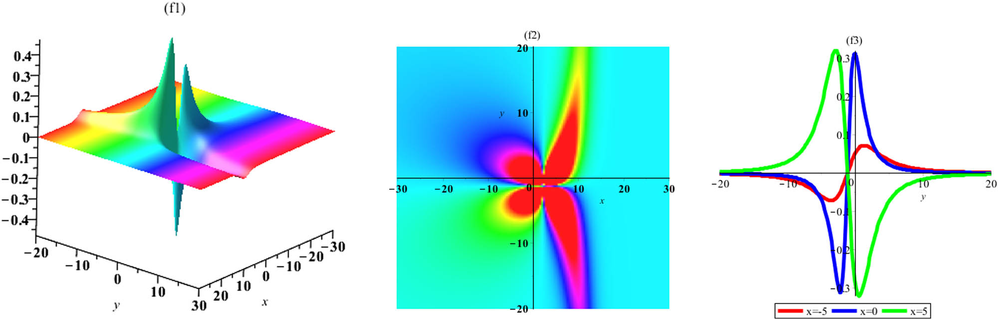
This section presents graphical representations of some obtained solutions. The 3D-surface graphs, 2D-density graphs, and 2D-line graphs of retrieved solutions are plotted using Maple software. In plotted graphs, (f1), (f2), (f3) represent the 3D-surface graphs, 2D-density graphs, and 2D-line graphs, respectively. The suitable numeric values are assigned to undetermined constants are presented earlier to generate the well-shaped graphs of obtained solutions. From the corresponding sets of obtained solutions, the considered values can be taken for plotting the graphs of acquired solutions. The acquired solutions of are graphically presented in Figures 1–26. The graphical representations include lump-1 soliton, lump-2 soliton, lump-3 soliton, and lump-4 soliton solutions. The graphs exhibit the effect of variation in the fractional parameter on the obtained solutions. The evolution of a lump-1 soliton is shown corresponding to the solution Eq. (2.5) through Figures 1 and 2 by choosing the values of selected parameters. Graphical simulations for the lump-1 soliton solution Eq. (2.7) are presented in Figures 3 and 4. The evolution of lump-2 soliton solution is illustrated from Figures 5 to 6, which has been obtained corresponding to the solution for Eq. (2.10). Also, graphical simulations for the lump-2 soliton solution Eq. (2.13) are presented in Figures 7 and 8. The evolution of lump-combined 2 soliton solution is illustrated in Figures 9 to 10, which has been obtained corresponding to the solution for Eq. (2.19). Also, the graphical simulations for the lump-combined 2 soliton solution Eq. (2.22) are presented in Figures 11 and 12. Moreover, the graphical simulations for the lump-combined 2 soliton solution Eq. (2.25) are shown in Figures 13 and 14. In another form, the graphical simulations for the lump-combined 2 soliton solution Eq. (2.28) are offered in Figures 15 and 16. The graphical simulations for the lump-3 soliton solution Eqs. (2.33), (2.35) and (2.37) are shown in Figures 17 and 18, Figures 19 and 20, and Figures 21 and 22, respectively. Finally, the graphical simulations for the lump-4 soliton solution Eqs. (2.42) and (2.45) are presented in Figures 23 and 24 and Figure 25 and 26, respectively. It is evident that the amplitude of the wave varies from one asymptotic state to another in each one of the mentioned cases for the lump-k soliton.

4 Conclusion

The (2+1)-dimensional KdV equation was studied in the current work, and the lump-N soliton wave solutions of the mentioned system were reached productively by the impressive multidimensional BBPs. The main contribution was to find the lump with k-soliton solutions. We investigated the analytical behavior of the obtained solutions by assigning appropriate values to the free-involved parameters. These new results were studied by using of a new method based on the Hirota bilinear technique. Besides, the bilinear form was obtained, and the N-soliton solutions were established. On top of that, lump-one, two, three, and four soliton solutions and multiwave solutions of the addressed system with known coefficients were presented. Some characteristics of the solutions were analyzed by visualizing the solutions. Also, the graphical illustrations of the solutions are provided. The solutions derived in this study were verified and genuinely beneficial for nonlinear scientific applications. The lump-soliton solutions will be useful additions to the literature for understanding related physical systems. In future, the nonlinear KdV model can also be investigated by other nonlinearity laws and the exact methods.

Acknowledgments

The Construction of Linear Algebra Teachers under the Hybrid Teaching Model.

Funding information: The authors state no funding involved.
Author contributions: X.W. and J. M.: methodology and software; G.S.: resources; J.M.: supervision; B.E. and A.A.: writing; N.A.M.A.K. and A.A.: investigation; X.W. and J. M.: software. All authors have read and agreed to the published version of the manuscript.
Conflict of interest: The authors state no conflict of interest.

References

[1] Manafian J, Lakestani M. Abundant soliton solutions for the Kundu-Eckhaus equation via tan(ϕ∕2)-expansion method. Optik. 2016;127:5543–51. 10.1016/j.ijleo.2016.03.041. Search in Google Scholar

[2] Ali NH, Mohammed SA, Manafian J. New explicit soliton and other solutions of the Van der Waals model through the ESHGEEM and the IEEM. J Modern Tech Eng. 2023;8:5–18. Search in Google Scholar

[3] Venkatesh N, Suresh P, Gopinath M, Naik MR. Design Of Environmental Monitoring System in Farm House Based on Zigbee. Int J Commun Comput Tech. 2022;10:1–4. 10.31838/ijccts/10.02.01. Search in Google Scholar

[4] Sun LY, Manafian J, Ilhan OA, Abotaleb M, Oudah AY, Prakaash AS. Theoretical analysis for miscellaneous soliton waves in metamaterials model by modification of analytical solutions. Opt Quant Elec. 2022;54:651. 10.1007/s11082-022-04033-8. Search in Google Scholar

[5] Li H, Peng R, Wang Z. On a diffusive susceptible-infected-susceptible epidemic model with mass action mechanism and birth-death effect: analysis, simulations, and comparison with other mechanisms. SIAM J Appl Math. 2018;78(4):2129–53. 10.1137/18M1167863. Search in Google Scholar

[6] Li R, Manafian J, Lafta HA, Kareem HA, Uktamov KF, Abotaleb M. The nonlinear vibration and dispersive wave systems with cross-kink and solitary wave solutions. Int J Geomet Meth Modern Phys. 2022;19:2250151. 10.1142/S0219887822501511. Search in Google Scholar

[7] Li R, Bu Sinnah ZA, Shatouri ZM, Manafian J, Aghdaei MF, Kadi A. Different forms of optical soliton solutions to the Kudryashovas quintuple self-phase modulation with dual-form of generalized nonlocal nonlinearity. Results Phys. 2023;46:106293. 10.1016/j.rinp.2023.106293 Search in Google Scholar

[8] Adel M, Aldwoah K, Alahmadi F, Osman MS. The asymptotic behavior for a binary alloy in energy and material science: The unified method and its applications. J Ocean Eng Sci. 2022. 10.1016/j.joes.2022.03.006. Search in Google Scholar

[9] Jin H, Wang Z. Boundedness, blowup and critical mass phenomenon in competing chemotaxis. J Diff Eq. 2016;260(1):162–96. 10.1016/j.jde.2015.08.040. Search in Google Scholar

[10] Hong X, Alkireet IA, Ilhan OA, Manafian J, Nasution MKM. Multiple soliton solutions of the generalized Hirota–Satsuma-Ito equation arising in shallow water wave. J Geom Phys. 2021;26:104338. 10.1016/j.geomphys.2021.104338. Search in Google Scholar

[11] Yang JY, Ma WX. Lump solutions to the bKP equation by symbolic computation. Int J Modern Phys B 2016;30:1640028. 10.1142/S0217979216400282. Search in Google Scholar

[12] Li Z, Manafian J, Ibrahimov N, Hajar A, Nisar KS, Jamshed W. Variety interaction between k-lump and k-kink solutions for the generalized Burgers equation with variable coefficients by bilinear analysis. Results Phys. 2021;28:104490. 10.1016/j.rinp.2021.104490. Search in Google Scholar

[13] Della Volpe C, Siboni S. From van der Waals equation to acid–base theory of surfaces: A chemical-mathematical journey. Rev Adhesion Adhesives. 2022;10:47–97. Search in Google Scholar

[14] Zhen L. Research on mathematical teaching innovation strategy and best practices based on deep learning algorithm. J Commer Biotech. 2022;27(3):180. 10.5912/jcb1284Search in Google Scholar

[15] Cao B, Gu Y, Lv Z, Yang S, Zhao J, Li Y. RFID reader anticollision based on distributed parallel particle swarm optimization. IEEE Internet Things J. 2021;8(5):3099–107. 10.1109/JIOT.2020.3033473. Search in Google Scholar

[16] Li Y, Zhou X. Image processing and flow field reconstruction algorithm of fluid trajectory in pipeline. Rev Adhesion Adhesives. 2022;10(2). Search in Google Scholar

[17] Dong J, Hu J, Zhao Y, Peng Y. Opinion formation analysis for Expressed and Private Opinions (EPOs) models: Reasoning private opinions from behaviors in group decision-making systems. Expert Sys. Appl. 2023;121292. 10.1016/j.eswa.2023.12.1292. Search in Google Scholar

[18] Srinivasareddy RS, Narayana DRYV, Krishna DRD. Sector beam synthesis in linear antenna arrays using social group optimization algorithm. National J Antennas Prop. 2021;3(2):6–9. 10.31838/NJAP/03.02.02Search in Google Scholar

[19] Wang Z, Fathollahzadeh Attar N, Khalili K, Behmanesh J, Band SS, Mosavi A, Chau KW. Monthly streamflow prediction using a hybrid stochastic-deterministic approach for parsimonious nonlinear time series modeling. Eng Appl Comput Fluid Mech. 2020;14(1):1351–72. 10.1080/19942060.2020.1830858. Search in Google Scholar

[20] Mohammadzadeh A, Castillo O, Band SS, Mosavi A. A novel fractional-order multiple-model type-3 fuzzy control for nonlinear systems with unmodeled dynamics. Int J Fuzzy Sys. 2021;23(6):1633–51. 10.1007/s40815-021-01058-1. Search in Google Scholar

[21] Manafian J, Lakestani M. N-lump and interaction solutions of localized waves to the (2+1)-dimensional variable-coefficient Caudrey-Dodd-Gibbon-Kotera-Sawada equation. J Geo Phys. 2020;150:03598. 10.1016/j.geomphys.2020.103598. Search in Google Scholar

[22] Madvar HR, Dehghani M, Memarzadeh R, Salwana E, Mosavi A, Shahab S. Derivation of optimized equations for estimation of dispersion coefficient in natural streams using hybridized ANN with PSO and CSO algorithms. IEEE Access. 2020;8:156582–99. 10.1109/access.2020.3019362. Search in Google Scholar

[23] Aslanova F. A comparative study of the hardness and force analysis methods used in truss optimization with metaheuristic algorithms and under dynamic loading. J Research Sci Eng Tech. 2020;8:25–33. 10.24200/jrset.vol8iss1pp25-33. Search in Google Scholar

[24] Li L, Duan C, Yu F. An improved Hirota bilinear method and new application for a nonlocal integrable complex modified Korteweg-de Vries (MKdV) equation. Phys Let A. 2019;383:1578–82. 10.1016/j.physleta.2019.02.031. Search in Google Scholar

[25] Cai W, Mohammaditab R, Fathi G, Wakil K, Ebadi AG, Ghadimi N. Optimal bidding and offering strategies of compressed air energy storage: A hybrid robust-stochastic approach. Renew Energy. 2019;143:1–8. 10.1016/j.renene.2019.05.008Search in Google Scholar

[26] Chen H. Hadronic molecules in B decays. Phys Review D. 2022;105(9):94003. 10.1103/PhysRevD.105.094003. Search in Google Scholar

[27] Chen H, Chen W, Liu X, Liu X. Establishing the first hidden-charm pentaquark withstrangeness. Eur Phys J C. 2021;81(5):409. 10.1140/epjc/s10052-021-09196-4. Search in Google Scholar

[28] Han E, Ghadimi N. Model identification of proton-exchange membrane fuel cells based on a hybrid convolutional neural network and extreme learning machine optimized by improved honey badger algorithm. Sustainable Energy Tech Assess. 2022;52:102005. Search in Google Scholar

[29] Zhang J, Khayatnezhad M, Ghadimi N. Optimal model evaluation of the proton-exchange membrane fuel cells based on deep learning and modified African vulture optimization algorithm. Energy Sources Part A Recovery Util Environ Eff 2022;44:287–305. 10.1080/15567036.2022.2043956Search in Google Scholar

[30] Yu D, Zhang T, He G, Nojavan S, Jermsittiparsert K, Ghadimi N. Energy management of wind-PV-storage-grid based large electricity consumer using robust optimization technique. J Energy Storage 2020;27:101054. 10.1016/j.est.2019.101054Search in Google Scholar

[31] Saeedi M, Moradi M, Hosseini M, Emamifar A, Ghadimi N., Robust optimization based optimal chiller loading under cooling demand uncertainty. Appl Therm Eng. 2019;148:1081–91. 10.1016/j.applthermaleng.2018.11.122Search in Google Scholar

[32] Aghazadeh MR, Asgari T, Shahi A, Farahm A. Designing strategy formulation processing model of governmental organizations based on network governance. Quart J Public Organiz Manag. 2016;4(1):29–52. Search in Google Scholar

[33] Gholamiangonabadi D, Nakhodchi S, Jalalimanesh A, Shahi A. Customer churnprediction using a meta-classifier approach; A case study of Iranian banking industry. Proceedings of the International Conference on Industrial Engineering and Operations Management Bangkok, Thailand, March 5–7, 2019.Search in Google Scholar

[34] Chen L, Huang H, Tang P, Yao D, Yang H, Ghadimi N. Optimal modeling of combined cooling, heating, and power systems using developed African Vulture Optimization: a case study in watersport complex. Energy Sources Part A Recovery Util Environ Eff. 2022;44:4296–317. 10.1080/15567036.2022.2074174Search in Google Scholar

[35] Jiang W, Wang X, Huang H, Zhang D, Ghadimi N. Optimal economic scheduling of microgrids considering renewable energy sources based on energy hub model using demand response and improved water wave optimization algorithm. J Energy Storage. 2022;55:105311. 10.1016/j.est.2022.105311Search in Google Scholar

[36] Dongmin Y, Ghadimi N. Reliability constraint stochastic UC by considering the correlation of random variables with Copula theory. IET Renew Power Gener. 2019;13(14):2587–93. 10.1049/iet-rpg.2019.0485Search in Google Scholar

[37] Mehrpooya M, Ghadimi N, Marefati M, Ghorbanian SA. Numerical investigation of a new combined energy system includes parabolic dish solar collector, stirling engine and thermoelectric device. Int J Energy Res. 2021;45(11):16436–55. 10.1002/er.6891Search in Google Scholar

[38] Erfeng H, Ghadimi N. Model identification of proton-exchange membrane fuel cells based on a hybrid convolutional neural network and extreme learning machine optimized by improved honey badger algorithm. Sustain Energy Tech Asses. 2022;52:102005. 10.1016/j.seta.2022.102005Search in Google Scholar

[39] Yuan Z, Wang W, Wang H, Ghadimi N. Probabilistic decomposition-based security constrained transmission expansion planning incorporating distributed series reactor. IET Gener. Trans Distrib. 2020;14(17):3478–87. 10.1049/iet-gtd.2019.1625Search in Google Scholar

[40] Mir M, Shafieezadeh M, Heidari MA, Ghadimi N. Application of hybrid forecast engine based intelligent algorithm and feature selection for wind signal prediction. Evolv Sys. 2020;11(4):559–73. 10.1007/s12530-019-09271-ySearch in Google Scholar

[41] Ma WX. Lump solutions to the Kadomtsev–Petviashvili equation. Phys Lett A. 2015;379:1975–8. 10.1016/j.physleta.2015.06.061. Search in Google Scholar

[42] Zhao N, Manafian J, Ilhan OA, Singh G, Zulfugarova R. Abundant interaction between lump and k-kink, periodic and other analytical solutions for the (3+1)-D Burger system by bilinear analysis. Int J Modern Phys B. 2021;35(13):2150173. 10.1142/S0217979221501733Search in Google Scholar

[43] Akter S, Hafez MG. Collisional positron acoustic soliton and double layer in an unmagnetized plasma having multi-species. Sci Reports. 2022;12:6453. 10.1038/s41598-022-10236-6Search in Google Scholar PubMed PubMed Central

[44] Ma WX. Interaction solutions to Hirota–Satsuma-Ito equation in (2+1)-dimensions. Front Math China. 2019;14:619–29. 10.1007/s11464-019-0771-ySearch in Google Scholar

[45] Ma WX. A search for lump solutions to a combined fourth order nonlinear PDE in (2+1)-dimensions. J Appl Anal Comput. 2019;9:1319–32. Search in Google Scholar

[46] Sun YL, Ma WX, Yu JP. N-soliton solutions and dynamic property analysis of a generalized three-component Hirota–Satsuma coupled KdV equation. Appl Math Let. 2021;120:107224. 10.1016/j.aml.2021.107224Search in Google Scholar

[47] Ma WX. N-soliton solution and the Hirota condition of a (2+1)-dimensional combined equation, Math. Comput. Simul. 2021;190:270–9. 10.1016/j.matcom.2021.05.020Search in Google Scholar

[48] Boiti M, Leon J, Pempinelli F. On the spectral transform of a Korteweg-de Vries equation in two space dimensions. Inverse Probl. 1985;2(3):271–9. 10.1088/0266-5611/2/3/005Search in Google Scholar

[49] Liu CF, Dai ZD. Exact periodic solitary wave and double periodic wave solutions for the (2.1)-dimensional Korteweg-de Vries equation. Z. Fr Naturfors A. 2009;64:609–14. 10.1515/zna-2009-9-1011Search in Google Scholar

[50] Lou SY. Generalized dromion solutions of the (2+1)-dimensional KdV equation. J Phys A: Math Gen. 1995;28:7227–32. 10.1088/0305-4470/28/24/019Search in Google Scholar

[51] Lou SY, Ruan HY. Revisitation of the localized excitations of the (2+1)-dimensional KdV equation. J Phys A: Math Gen. 2001;34:305–16. 10.1088/0305-4470/34/2/307Search in Google Scholar

[52] Wazwaz AM Solitons and singular solitons for the Gardner-KP equation. Appl Math Comput. 2008;204:162–9. 10.1016/j.amc.2008.06.011Search in Google Scholar

[53] Wang CJ, Dai ZD, Lin L. Exact three-wave solution for higher dimensional KdV-type equation. Appl Math Comput. 2010;216:501–5. 10.1016/j.amc.2010.01.057Search in Google Scholar

[54] Liu JG, Ye Q. Exact periodic cross-kink wave solutions for the (2+1)-dimensional Korteweg-de Vries equation. Anal Math Phys. 2020;10:54. 10.1007/s13324-020-00397-wSearch in Google Scholar

[55] Liu J, Mu G, Dai Z, Luo H. Spatiotemporal deformation of multi-soliton to (2+1)-dimensional KdV equation. Nonlinear Dyn. 2016;83:355–60. 10.1007/s11071-015-2332-6Search in Google Scholar

[56] Liu JG. Lump-type solutions and interaction solutions for the (2+1)-dimensional asymmetrical Nizhnik-Novikov-Veselov equation. Eur Phys J Plus. 2019;134:56. 10.1140/epjp/i2019-12470-0Search in Google Scholar

[57] Ilhan OA, Manafian J, Alizadeh A, Mohammed SA. M lump and interaction between M lump and N stripe for the third-order evolution equation arising in the shallow water. Adv Diff Equ. 2020;207:2020. 10.1186/s13662-020-02669-ySearch in Google Scholar

[58] Shen G, Manafian J, Huy DTN, Nisar KS, Abotaleb M, Trung ND. Abundant soliton wave solutions and the linear superposition principle for generalized (3+1)-D nonlinear wave equation in liquid with gas bubbles by bilinear analysis. Results Phys. 2022;32:105066. 10.1016/j.rinp.2021.105066Search in Google Scholar

[59] Gang W, Manafian J, Benli FB, Ilhan OA, Goldaran R. Modulational instability and multiple rogue wave solutions for the generalized CBS?BK equation. Modern Phys Let B. 2021;35(24):2150408. 10.1142/S021798492150408XSearch in Google Scholar

[60] Zhao Z, He L. M-lump and hybrid solutions of a generalized (2+1)-dimensional Hirota–Satsuma-Ito equation. Appl Math Let. 2021;111:106612. 10.1016/j.aml.2020.106612Search in Google Scholar

[61] He L, Zhang J, Zhao Z. Resonance Y-type soliton, hybrid and quasi-periodic wave solutions of a generalized (2+1)-dimensional nonlinear wave equation. Nonlinear Dyn. 2021;106:2515–35. 10.1007/s11071-021-06922-1Search in Google Scholar

[62] Tan W, Zhang W, Zhang J. Evolutionary behavior of breathers and interaction solutions with M-solitons for (2+1)-dimensional KdV system. Appl Math Let. 2020;101:106063. 10.1016/j.aml.2019.106063Search in Google Scholar

[63] Tan W. Evolution of breathers and interaction between high-order lump solutions and N-solitons (Nrightarrow infty) for Breaking Soliton system. Phys Let A. 2019;383:125907. 10.1016/j.physleta.2019.125907Search in Google Scholar

[64] Tan W, Dai ZD, Yin ZY. Dynamics of multi-breathers, N-solitons and M-lump solutions in the (2+1)-dimensional KdV equation. Nonlinear Dyn. 2019;96:1605–14. 10.1007/s11071-019-04873-2Search in Google Scholar

[65] Liu Y, Ren B, Wang DS. Localized nonlinear wave interaction in the generalised Kadomtsev–Petviashvili equation. East Asian J Appl Math. 2021;11(2):301–25. 10.4208/eajam.290820.261020Search in Google Scholar

[66] Cheng L, Ma WX, Zhang Y, Ge JY. Integrability and lump solutions to an extended (2+1)-dimensional KdV equation. Eur Phys J Plus. 2022;137:902. 10.1140/epjp/s13360-022-03076-wSearch in Google Scholar

[67] Gaur M, Singh K. Lie group of transformations for time fractional Gardner equation. AIP Conf Proc. 2022;2357:090006. 10.1063/5.0080583Search in Google Scholar

[68] Aneja M, Gaur M, Bose T, Gantayat PK, Bala R. Computer-based numerical analysis of bioconvective heat and mass transfer across a nonlinear stretching sheet with hybrid nanofluids. In: Bhateja V, Yang XS, Ferreira MC, Sengar SS, Travieso-Gonzalez CM. (eds). Evolution in Computational Intelligence. FICTA 2023. Smart Innovation, Systems and Technologies. vol 370. Singapore: Springer; 2023. 10.1007/978-981-99-6702-5_55. Search in Google Scholar

[69] Safi Ullah M, Ali MZ, Harun-Or Roshid, Hoque MF. Collision phenomena among lump, periodic and stripe soliton solutions to a (2+1)-dimensional Benjamin–Bona–Mahony–Burgers Model. Eur Phys J Plus. 2021;136:370. 10.1140/epjp/s13360-021-01343-wSearch in Google Scholar

[70] Roshid MM, Bairagi T, Harun-Or Roshid, Rahman MM. Lump, interaction of lump and kink and solitonic solution of nonlinear evolution equation which describe incompressible viscoelastic Kelvin–Voigt fluid. Partial Differ Equ Appl Math. 2022;5:100354. 10.1016/j.padiff.2022.100354Search in Google Scholar

[71] Kumar S, Almusawa H, Kumar A. Some more closed-form invariant solutions and dynamical behavior of multiple solitons for the (2+1)-dimensional rdDym equation using the Lie symmetry approach. Results Phys. 2021;24:104201. 10.1016/j.rinp.2021.104201Search in Google Scholar

[72] Kumar S, Kumar D, Kharbanda H. Lie symmetry analysis, abundant exact solutions and dynamics of multisolitons to the (2+1)-dimensional KP-BBM equation. Pramana. 2021;85:33. 10.1007/s12043-020-02057-xSearch in Google Scholar

[73] Kumar S, Kumar D. Lie symmetry analysis and dynamical structures of soliton solutions for the (2+1)-dimensional modified CBS equation. Int J Modern Phys B. 2020;34(25):2050221. 10.1142/S0217979220502215Search in Google Scholar

[74] Li R, Ilhan OA, Manafian J, Mahmoud KH, Abotaleb M, Kadi A. A mathematical study of the (3+1)-D variable coefficients generalized shallow water wave equation with its application in the interaction between the lump and soliton solutions. Math. 2022;10(17):3074. 10.3390/math10173074Search in Google Scholar

[75] Li J, Manafian J, Wardhana A, Othman AJ, Husein I, Al-Thamir M, Abotaleb M. N-lump to the (2+1)-dimensional variable-coefficient Caudrey-Dodd-Gibbon-Kotera-Sawada equation. Complexity. 2022;2022:4383100. 10.1155/2022/4383100Search in Google Scholar

[76] Zhou X, Ilhan OA, Zhou F, Sutarto S, Manafian J, Abotaleb M. Lump and interaction solutions to the (3+1)-dimensional variable-coefficient nonlinear wave equation with multidimensional binary bell polynomials. J Funct Spaces. 2021;2021:4550582. 10.1155/2021/4550582Search in Google Scholar

Received: 2023-08-27

Revised: 2023-12-04

Accepted: 2023-12-05

Published Online: 2023-12-31

This work is licensed under the Creative Commons Attribution 4.0 International License.

Articles in the same Issue

https://doi.org/10.1515/phys-2023-0167

Keywords for this article

Hirota bilinear scheme; (2+1)-dimensional KdV equation; interaction lump with k-soliton solutions

Creative Commons

BY 4.0