Some standard and nonstandard finite difference schemes for a reaction–diffusion–chemotaxis model
-
 and
and

Abstract
Two standard and two nonstandard finite difference schemes are constructed to solve a basic reaction–diffusion–chemotaxis model, for which no exact solution is known. The continuous model involves a system of nonlinear coupled partial differential equations subject to some specified initial and boundary conditions. It is not possible to obtain theoretically the stability region of the two standard finite difference schemes. Through running some numerical experiments, we deduce heuristically that these classical methods give reasonable solutions when the temporal step size
Nomenclature
- conc.
-
concentration
- pop.
-
population
- PDE
-
partial differential equation
- SFD
-
standard finite difference
- NSFD
-
nonstandard finite difference
-
-
temporal step size
-
-
spatial step size
-
-
time level
-
-
space level
-
-
population of bacteria
-
-
food concentration
-
-
approximation for population of bacteria
-
-
approximation for food concentration
-
-
diffusion coefficient of the cells
-
-
diffusion coefficient of the attractants
-
-
chemotactic term
-
-
spontaneous production coefficient of attractant
-
-
decay coefficient of attractant activity
-
1 Introduction
Diffusion equations are often in the form of reaction–diffusion and advection–diffusion, which have been well studied in the modeling of biological processes [1]. Advection–diffusion models are often used in the field of oceanography to study ocean tracers, such as large-scale ocean circulation [2]. Reaction–diffusion processes can be widely observed in nature, notably in the formation and spread of patterns such as spots and stripes over the surface of animals through the chemical interaction between cells [3]. Unlike reaction–diffusion and advection–diffusion, the mathematical analysis for cross-diffusion equations is a challenge that is largely underdeveloped [1]. Cross-diffusion arises when the concentration gradient of one species induces the flux of another species [4]. Cross-diffusion equations are fundamental in the modeling of several natural processes such as cancer growth [5], population dynamics via Volterra–Lotka cross-diffusion systems [6] and chemotaxis [7]. Theoretically, equations consisting of cross-diffusion terms are challenging largely due to being strongly coupled nonlinear parabolic systems that do not enjoy the maximum principle, and thus, deriving appropriate estimates and proving the existence of positive solutions are not easy [1]. However, in refs [8] and [9], some results on global and local existence of solutions as well as on their long-time behaviour have been established. Recently, some results on the existence and uniqueness of solutions (wellposedness) were obtained in refs [10] and [11]. Standard finite difference (SFD) methods lack the ability to preserve positivity; in contrast, the numerical solutions from nonstandard finite difference (NSFD) methods can preserve properties from the exact solution when solving a differential equation, and this makes NSFD methods appealing [12]. Ronald E. Mickens started to work on NSFD methods around 1990. Another advantage of NSFD over classical methods for reaction–diffusion equations is that classical methods can experience blow up at long propagation time [13,14]. Studying the stability is not easy for classical finite difference methods discretising nonlinear partial differential equations (PDEs). The freezing coefficient technique and von Neumann stability analysis can be used, but freezing coefficient is not a very accurate technique.
NSFD methods are very popular to solve reaction–diffusion PDEs. For reaction–diffusion equations, we can obtain conditions for which NSFD methods are positivity preserving and we can prove boundedness [15]. Positivity and boundedness will ensure stability [15]. It is also difficult to study properties such as stability due to the nature of cross-diffusion systems when SFD methods are used. NSFD schemes are constructed by using some fundamental principles [16]:
The denominator of the discrete derivative must be replaced by a more general function, for example,
In general, we use non-local representation of nonlinear terms [17], for example,
The difference equation should have the same order as the original equation. In general, when the order of the difference equation is larger than the order of the differential equation, spurious solutions might appear as discussed in ref. [18].
The discrete approximation should preserve some important properties of the corresponding differential equation. Properties such as boundedness and positivity should be preserved [19].
This article is presented as follows. In Section 2, we describe the basic reaction–diffusion–chemotaxis model to be solved, and we also give some discussion on how the numerical rate of convergence can be calculated in Section 3. Section 4 is dedicated to the two standard schemes SFD1 and SFD2 to solve the reaction–diffusion–chemotaxis model. In Sections 4.3 and 4.4, we present some numerical results. Sections 5 and 6 are dedicated to the two nonstandard schemes NSFD1 and NSFD2 to solve the reaction–diffusion–chemotaxis model. In Section 5.1, we describe the NSFD1 scheme and check the consistency. We present some numerical results in 5.2 for NSFD1. In Section 6.1, we describe NSFD2 scheme [1], and we also check the consistency. In Section 6.2, some numerical results are presented for NSFD2. In Section 7, we give some concluding remarks.
2 The basic reaction–diffusion–chemotaxis model
Chemotaxis refers to the chemically directed movement of a bacterial population
The mathematical model for the basic reaction–diffusion–chemotaxis model proposed in ref. [7], is described as follows:
where
The parameters
Since Eq. (1) contains
We consider the following initial conditions given in [1]:
We will work with the spatial domain
The parameters are chosen as follows:
Case 1:
Case 2:
We have considered case 2, as one of the conditions for positivity of NSFD1 is that
3 Analysis of convergence
As we do not have an analytical solution, we obtain the numerical rate of convergence in time by using
where
All numerical simulations are done in MATLAB using an Intel Core i5-10600k with 16GB RAM.
4 Classical methods to solve the reaction–diffusion–chemotaxis model
4.1 SFD1 to solve the continuous model
We construct SFD1 by using forward difference approximation for
and
where
Rewriting Eqs. (4) and (5) yields
and
To check for consistency and to obtain the order of accuracy of SFD1 scheme, we obtain the Taylor series expansion of Eqs. (6) and (7) about the point
and
As
and
We therefore conclude that SFD1 scheme is consistent with the PDEs given by Eqs. (1) and (2). The scheme is first-order accurate in time.
4.2 SFD2 to solve the continuous model
We construct SFD2 by using forward difference approximation for
Eq. (2) is discretised in a similar way as in SFD1. We therefore have
and
We now check for consistency and obtain the order of accuracy of SFD2 scheme. From the Taylor series expansion of Eqs. (7) and (9) about the point
and
As
and
We conclude that SFD2 scheme is consistent with the PDEs given by Eqs. (1) and (2). The scheme is first-order accurate in time and second order accurate in space.
4.3 Numerical results for SFD1 and SFD2: Case 1
Stability analysis using the Von Neumann condition cannot be used for the two standard schemes as the equations are coupled. We note that
The same approach is used to obtain some values of
In Tables 1 and 2, the numerical rate of convergence in time is obtained using SFD1 and SFD2 for case 1, and we conclude that the order of convergence in time is one.
|
|
|
|
|
|
|---|---|---|---|---|
|
|
|
|
||
|
|
|
|
1.0408 | 0.9801 |
|
|
|
|
1.0206 | 0.9909 |
|
|
|
|
1.0103 | 0.9957 |
|
|
|
|
|
|
|---|---|---|---|---|
|
|
|
|
||
|
|
|
|
1.0388 | 0.9950 |
|
|
|
|
0.8141 | 0.9975 |
|
|
|
|
0.9160 | 0.9988 |
4.3.1 SFD1 (case 1)

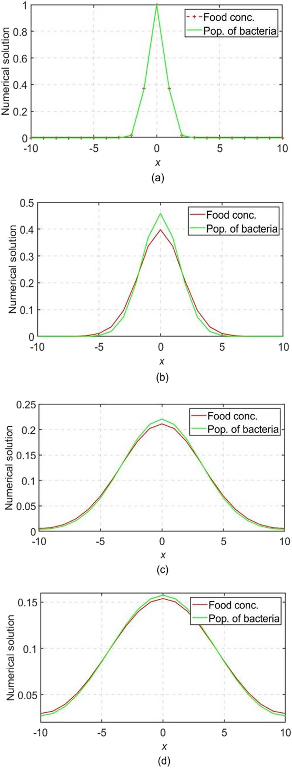
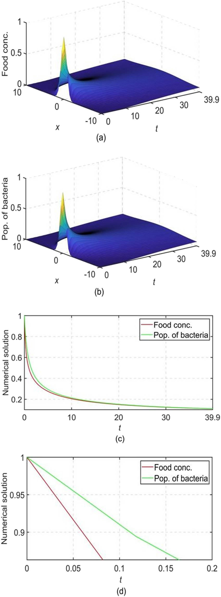
Results for the chemotaxis model using SFD1 for case 1 with

Results for the chemotaxis model using SFD1 for case 1 with

Results for the chemotaxis model using SFD1 for case 1 with

Plot of numerical solutions vs
4.3.2 SFD2 (case 1)

Results for the chemotaxis model using SFD2 for case 1 with

Results for the chemotaxis model using SFD2 for case 1 with

Plot of numerical solutions vs
4.3.3 Numerical rate of convergence in time for SFD1 and SFD2: Case 1
4.4 Numerical results for SFD1 and SFD2: case 2
The same approach as discussed in Section 4.3 is used to display numerical solutions using SFD1 and SFD2 for case 2.
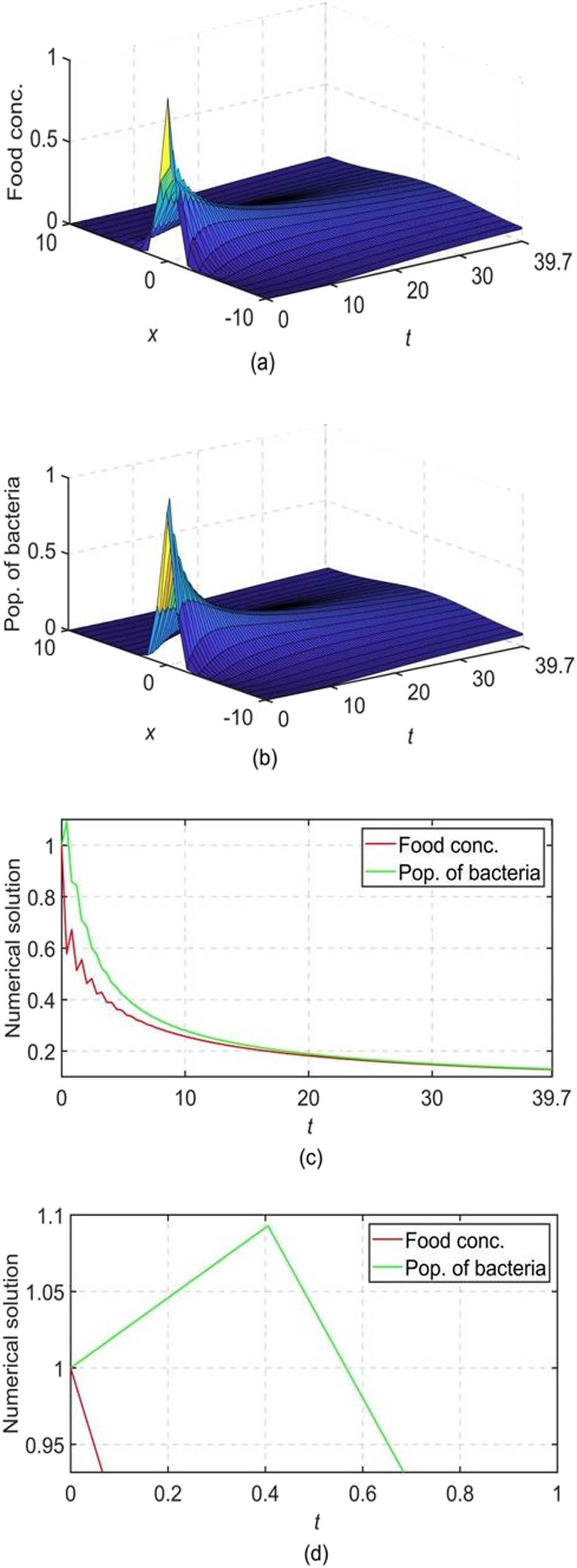
We present results in Figures 8, 9 and 10 using SFD1 and SFD2 and we observe that the numerical solutions are bounded and free of dispersive oscillations. We observe no overshoot, unlike those of case 1 (see Figures 3 and 6).
Figures 11 and 12 show the plot of the numerical solutions vs
We obtain the numerical rate of convergence in time using SFD1 and SFD2 for case 2 in Tables 3 and 4. We conclude that the order of convergence in time is one for both standard schemes.
|
|
|
|
|
|
|---|---|---|---|---|
|
|
|
|
||
|
|
|
|
1.0212 | 0.9953 |
|
|
|
|
1.0105 | 0.9983 |
|
|
|
|
|
|
|---|---|---|---|---|
|
|
|
|
||
|
|
|
|
1.0210 | 0.9949 |
|
|
|
|
1.0104 | 0.9981 |
4.4.1 SFD1 (case 2)

Results for the chemotaxis model using SFD1 for case 2 with

Results for the chemotaxis model using SFD1 for case 2 with

Results for the chemotaxis model using SFD2 for case 2 with
4.4.2 SFD2 (Case 2)

Plot of numerical solutions vs
Plot of numerical solutions vs
4.4.3 Numerical rate of convergence in time for SFD1 and SFD2: case 2
5 NSFD method to solve the reaction–diffusion–chemotaxis model
The logistic equation is the space independent case of
which is
An exact scheme constructed in [20] to discretise
where
5.1 NSFD1
Anguelov et al. [27] discretised the Fisher-Kolmogorov-Petrovsky-Piskunov equation i.e.
where
We use the same discretisation for
This gives the following scheme referred to as NSFD1 for the continuous chemotaxis model:
and
where
Eq. (11) can be rewritten as follows:
or
We note that NSFD1 was derived by Chapwanya et al. [1] for the chemotaxis model, but they did not use the scheme to present results and also did not study the positivity and boundedness of the method as their aim was to modify NSFD1 to obtain a positivity preserving method.
For simplification, the following relation is used, namely,
Hence, Eqs. (12) and (13) give
and
We note that
and
and the initial conditions must be non-negative.
The scheme given by Eq. (15) preserves positivity of the continuous model if the initial conditions are non-negative, i.e.,
To check for consistency and to obtain the order of accuracy of NSFD1 scheme, we consider Eqs. (14) and (15) and the Taylor series expansions about the point
and
As
and
We, therefore, conclude that the NSFD1 scheme is consistent with the PDEs given by Eqs. (1) and (2). The scheme is first-order accurate in time.
5.2 Numerical results for NSFD1
5.2.1 Case 1
In the construction of NSFD1, the relationship
Since

Results for the chemotaxis model using NSFD1 with

Results for the chemotaxis model using NSFD1 with
5.2.2 Case 2
For case 2,
Since

Results for the chemotaxis model using NSFD1 with
Results for the chemotaxis model using NSFD1 with
We verify numerically that the order of convergence in time is one as displayed from calculations in Table 5.
|
|
|
|
|
|
|---|---|---|---|---|
|
|
|
|
||
|
|
|
|
1.0168 | 1.2404 |
|
|
|
|
0.9523 | 1.0274 |
6 Modification of NSFD1 scheme
6.1 NSFD2
Chapwanya et al. [1] derived NSFD2 by modifying NSFD1.
In NSFD2,
We start with Eq. (11), i.e.,
which can be rewritten as follows:
or
Chapwanya et al. [1] multiplied the negative term of the RHS of Eq. (16) by
Eq. (16) is modified to
The first equation for NSFD2 is therefore
where
From Eq. (12), we have
and using the functional relation
Theorem 1
NSFD2 preserves positivity of the continuous model if
Since
To check for consistency and to obtain the order of accuracy of NSFD2 scheme, we consider Eq. (18) and the Taylor series expansions about the point
As
We therefore conclude that NSFD2 scheme is not consistent with the PDE given by Eq. (1). We would like to mention that the consistency of NSFD2 was not checked in [1]. This is a novel result obtained.
From Eq. (19), we see that NSFD2 can be made consistent if
Choosing different combinations of
For
For
From Eqs. (20) and (21), we can deduce that the choices
6.2 Numerical results for NSFD2
We now present results for the two cases using NSFD2. The profiles from case 1 are not very informative as NSFD2 is not consistent for case 1.
We can choose the following combinations of
From Figures 17 and 18, we observe some overshoot and uneven profiles when case 1
Table 6 gives the maximum norm errors
|
|
|
|
|
|
|---|---|---|---|---|
|
|
|
|
||
|
|
|
|
1.0255 | 1.2438 |
|
|
|
|
0.9509 | 1.0284 |
6.2.1 Case 1
Results for the chemotaxis model using NSFD2 with

Results for the chemotaxis model using NSFD2 with
6.2.2 Case 2

Results for the chemotaxis model using NSFD2 with

Results for the chemotaxis model using NSFD2 with
7 Conclusion
In this work, two SFD methods and two NSFD methods were used to solve a basic reaction–diffusion–chemotaxis model consisting of a cross-diffusion term and a system of nonlinear coupled PDEs requiring positivity preserving numerical solutions. The standard methods SFD1 and SFD2 resulted in unreasonable numerical solutions at some combinations of values of
NSFD1 was not always positivity preserving depending on the parameters used. NSFD1 can be used when conditions for positivity hold, that is, when
Acknowledgments
The authors would like to thank the anonymous reviewers and editor for comments and suggestions that helped to improve the article considerably.
-
Funding information: G.N. de Waal would like to thank the department of Mathematics and Applied Mathematics of Nelson Mandela University for providing some funding toward his MSc studies. A.R. Appadu is grateful to Nelson Mandela University and the National Research Foundation of South Africa (Grant Number: 136161), which allowed this work to be carried out. C.J. Pretorius is grateful to the National Research Foundation of South Africa (Grant Number: 132544).
-
Author contributions: The plan of the work was provided by Appadu. Most derivation and analysis was done by de Waal under supervision of Appadu and Pretorius. All authors have accepted responsibility for the entire content of this manuscript and approved its submission.
-
Conflict of interest: The authors state no conflict of interest.
References
[1] Chapwanya M, Lubuma JM-S, Mickens RE. Positivity-preserving non-standard finite difference schemes for cross-diffusion equations in biosciences. Comput Math Appl. 2014;68(9):1071–82. 10.1016/j.camwa.2014.04.021. Search in Google Scholar
[2] Roy-Barman M, Jeandel C. Marine geochemistry: ocean circulation, carbon cycle and climate change. Online Edition. Oxford: Oxford Academic; 2016. p. 978-0191829604. 10.1093/acprof:oso/9780198787495.001.0001Search in Google Scholar
[3] Volpert V, Petrovskii S. Reaction-diffusion waves in biology. Phys Life Rev. 2009;6(4):267–310. 10.1016/j.plrev.2009.10.002. Search in Google Scholar PubMed
[4] Vanag, VK, Epstein, IV. Cross-diffusion and pattern formation in reaction–diffusion systems. Phys Chemistry Chem Phys 2009;11(6):897–912. 10.1039/B813825G. Search in Google Scholar PubMed
[5] Marchant BP, Norbury J, Perumpanani AJ. Traveling shock waves arising in a model of malignant invasion. SIAM J Appl Math. 2000;60(2):463–76. 10.1137/S0036139998328034. Search in Google Scholar
[6] Murray JD. Mathematical biology II: spatial models and biomedical applications. 3rd ed. New York: Springer; 2003. p. 978-038795228, 814. 10.1007/b98869Search in Google Scholar
[7] Murray JD. Mathematical biology I: an introduction. 3rd Ed. New York: Springer; 2002. 978-0387952239. p. 551. 10.1007/b98868Search in Google Scholar
[8] Chen L, Jüngel A. Analysis of a parabolic cross-diffusion population model without self-diffusion. J Differ Equ. 2006;60(1):39–59. 10.1016/j.jde.2005.08.002. Search in Google Scholar
[9] Le D. Cross-diffusion equations on n spatial dimensional domains. In: Fifth Mississippi State Conference on Differential Equations and Computational Simulations, Electron. J. Diff. Equ. Conference. vol. 10, 2003, Mississippi. p. 193–210. Search in Google Scholar
[10] Seis, S, Winkler, D. A well-posedness result for a system of cross-diffusion equations. J Evolut Equ. 2020;21:2471–89. 10.1007/S00028-021-00690-6. Search in Google Scholar
[11] Chen, L, Daus, ES, Jüngel, A. Global existence analysis of cross-diffusion population systems for multiple species. Archive Rational Mech Anal. 2018;227(2018):715–47. 10.1007/S00205-017-1172-6. Search in Google Scholar
[12] Mickens RE. Advances in the application of non-standard finite difference schemes. Singapore: World Scientific; 2005. p. 978-9812564047. 664. 10.1142/5884Search in Google Scholar
[13] Sun GF, Liu GR, Li M. An efficient explicit finite-difference scheme for simulating coupled biomass growth on nutritive substrates. Math Probl Eng. 2015;2015:1–17. 10.1155/2015/708497. Search in Google Scholar
[14] Sun GF, Liu GR, Li M. A novel explicit positivity preserving finite-difference scheme for simulating bounded growth of biological films. Int J Comput Meth. 2016;13(2):1640013. 10.1142/S0219876216400132. Search in Google Scholar
[15] Yu Y, Deng W, Wu Y. Positivity and boundedness preserving schemes from space-time fractional predator-prey reaction–diffusion model. Comp Math Appl. 2015;69(8):743–59. 10.1016/j.camwa.2015.02.024. Search in Google Scholar
[16] Mickens RE. Exact solutions to a finite-difference model of a nonlinear reaction-advection equation: implications for numerical analysis. Numer Meth Partial Differ Equ. 1989;5(4):313–25. 10.1002/num.1690050404. Search in Google Scholar
[17] Anguelov R, Lubuma JM-S. Contributions to the mathematics of the non-standard finite difference method and applications. Numer Methods Partial Differ Equ. 2001;17(5):518–43. 10.1002/num.1025. Search in Google Scholar
[18] Hildebrand FB. Finite-difference equations and simulations. New Jersey: Prentice-Hall; 1968. p. 978-0133172300, 338. Search in Google Scholar
[19] Mickens RE. Nonstandard finite difference models of differential equations. Singapore: World Scientific; 1994. p. 978-9810214586, 264. 10.1142/2081Search in Google Scholar
[20] Anguelov R, Lubuma JM-S. Nonstandard finite difference method by non-local approximation. Math Comput Simul. 2003;61(2003):465–75. 10.1016/S0378-4754(02)00106-4. Search in Google Scholar
[21] Mickens RE. Nonstandard finite difference models of differential equations. Singapore: World Scientific; 2000. p. 9978-981-4493-98-7, 664. Search in Google Scholar
[22] Bhatt HP, Khaliq AQM. Fourth-order compact schemes for the numerical simulation of coupled Burgers’ equation. Comput Phys Commun. 2015;200:117–38. 10.1016/j.cpc.2015.11.007Search in Google Scholar
[23] Tijani YO, Appadu AR, Aderogba AA. Some finite difference methods to model biofilm growth and decay: classical and non-standard. Comput. 2021;9(11):123. 10.3390/computation9110123. Search in Google Scholar
[24] Appadu AR, Tijani YO, Aderogba AA. On the performance of some NSFD methods for a 2-D generalized Burgers-Huxley equation. J Differ Equ Appl. 2021;27(11):1537–73. 10.1080/10236198.2021.1999433. Search in Google Scholar
[25] Tijani YO, Appadu AR. Unconditionally positive NSFD and classical finite difference schemes for biofilm formation on medical implant using Allen-Cahn equation. Demonstr Math. 2022;55(1):40–60. 10.1515/dema-2022-0006. Search in Google Scholar
[26] Kovel M, Zubik-Kowal B. Numerical solutions for a model of tissue invasion and migration of tumour cells. Comput Math Meth Med. 2010;2011:1–16. 10.1155/2011/452320. Search in Google Scholar PubMed PubMed Central
[27] Anguelov R, Kama P, Lubuma JM-S. On non-standard finite difference models of reaction–diffusion equations. J Comput Appl Math. 2005;175(1):11–29. 10.1016/j.cam.2004.06.002. Search in Google Scholar
© 2023 the author(s), published by De Gruyter
This work is licensed under the Creative Commons Attribution 4.0 International License.
Articles in the same Issue
- Regular Articles
- Dynamic properties of the attachment oscillator arising in the nanophysics
- Parametric simulation of stagnation point flow of motile microorganism hybrid nanofluid across a circular cylinder with sinusoidal radius
- Fractal-fractional advection–diffusion–reaction equations by Ritz approximation approach
- Behaviour and onset of low-dimensional chaos with a periodically varying loss in single-mode homogeneously broadened laser
- Ammonia gas-sensing behavior of uniform nanostructured PPy film prepared by simple-straightforward in situ chemical vapor oxidation
- Analysis of the working mechanism and detection sensitivity of a flash detector
- Flat and bent branes with inner structure in two-field mimetic gravity
- Heat transfer analysis of the MHD stagnation-point flow of third-grade fluid over a porous sheet with thermal radiation effect: An algorithmic approach
- Weighted survival functional entropy and its properties
- Bioconvection effect in the Carreau nanofluid with Cattaneo–Christov heat flux using stagnation point flow in the entropy generation: Micromachines level study
- Study on the impulse mechanism of optical films formed by laser plasma shock waves
- Analysis of sweeping jet and film composite cooling using the decoupled model
- Research on the influence of trapezoidal magnetization of bonded magnetic ring on cogging torque
- Tripartite entanglement and entanglement transfer in a hybrid cavity magnomechanical system
- Compounded Bell-G class of statistical models with applications to COVID-19 and actuarial data
- Degradation of Vibrio cholerae from drinking water by the underwater capillary discharge
- Multiple Lie symmetry solutions for effects of viscous on magnetohydrodynamic flow and heat transfer in non-Newtonian thin film
- Thermal characterization of heat source (sink) on hybridized (Cu–Ag/EG) nanofluid flow via solid stretchable sheet
- Optimizing condition monitoring of ball bearings: An integrated approach using decision tree and extreme learning machine for effective decision-making
- Study on the inter-porosity transfer rate and producing degree of matrix in fractured-porous gas reservoirs
- Interstellar radiation as a Maxwell field: Improved numerical scheme and application to the spectral energy density
- Numerical study of hybridized Williamson nanofluid flow with TC4 and Nichrome over an extending surface
- Controlling the physical field using the shape function technique
- Significance of heat and mass transport in peristaltic flow of Jeffrey material subject to chemical reaction and radiation phenomenon through a tapered channel
- Complex dynamics of a sub-quadratic Lorenz-like system
- Stability control in a helicoidal spin–orbit-coupled open Bose–Bose mixture
- Research on WPD and DBSCAN-L-ISOMAP for circuit fault feature extraction
- Simulation for formation process of atomic orbitals by the finite difference time domain method based on the eight-element Dirac equation
- A modified power-law model: Properties, estimation, and applications
- Bayesian and non-Bayesian estimation of dynamic cumulative residual Tsallis entropy for moment exponential distribution under progressive censored type II
- Computational analysis and biomechanical study of Oldroyd-B fluid with homogeneous and heterogeneous reactions through a vertical non-uniform channel
- Predictability of machine learning framework in cross-section data
- Chaotic characteristics and mixing performance of pseudoplastic fluids in a stirred tank
- Isomorphic shut form valuation for quantum field theory and biological population models
- Vibration sensitivity minimization of an ultra-stable optical reference cavity based on orthogonal experimental design
- Effect of dysprosium on the radiation-shielding features of SiO2–PbO–B2O3 glasses
- Asymptotic formulations of anti-plane problems in pre-stressed compressible elastic laminates
- A study on soliton, lump solutions to a generalized (3+1)-dimensional Hirota--Satsuma--Ito equation
- Tangential electrostatic field at metal surfaces
- Bioconvective gyrotactic microorganisms in third-grade nanofluid flow over a Riga surface with stratification: An approach to entropy minimization
- Infrared spectroscopy for ageing assessment of insulating oils via dielectric loss factor and interfacial tension
- Influence of cationic surfactants on the growth of gypsum crystals
- Study on instability mechanism of KCl/PHPA drilling waste fluid
- Analytical solutions of the extended Kadomtsev–Petviashvili equation in nonlinear media
- A novel compact highly sensitive non-invasive microwave antenna sensor for blood glucose monitoring
- Inspection of Couette and pressure-driven Poiseuille entropy-optimized dissipated flow in a suction/injection horizontal channel: Analytical solutions
- Conserved vectors and solutions of the two-dimensional potential KP equation
- The reciprocal linear effect, a new optical effect of the Sagnac type
- Optimal interatomic potentials using modified method of least squares: Optimal form of interatomic potentials
- The soliton solutions for stochastic Calogero–Bogoyavlenskii Schiff equation in plasma physics/fluid mechanics
- Research on absolute ranging technology of resampling phase comparison method based on FMCW
- Analysis of Cu and Zn contents in aluminum alloys by femtosecond laser-ablation spark-induced breakdown spectroscopy
- Nonsequential double ionization channels control of CO2 molecules with counter-rotating two-color circularly polarized laser field by laser wavelength
- Fractional-order modeling: Analysis of foam drainage and Fisher's equations
- Thermo-solutal Marangoni convective Darcy-Forchheimer bio-hybrid nanofluid flow over a permeable disk with activation energy: Analysis of interfacial nanolayer thickness
- Investigation on topology-optimized compressor piston by metal additive manufacturing technique: Analytical and numeric computational modeling using finite element analysis in ANSYS
- Breast cancer segmentation using a hybrid AttendSeg architecture combined with a gravitational clustering optimization algorithm using mathematical modelling
- On the localized and periodic solutions to the time-fractional Klein-Gordan equations: Optimal additive function method and new iterative method
- 3D thin-film nanofluid flow with heat transfer on an inclined disc by using HWCM
- Numerical study of static pressure on the sonochemistry characteristics of the gas bubble under acoustic excitation
- Optimal auxiliary function method for analyzing nonlinear system of coupled Schrödinger–KdV equation with Caputo operator
- Analysis of magnetized micropolar fluid subjected to generalized heat-mass transfer theories
- Does the Mott problem extend to Geiger counters?
- Stability analysis, phase plane analysis, and isolated soliton solution to the LGH equation in mathematical physics
- Effects of Joule heating and reaction mechanisms on couple stress fluid flow with peristalsis in the presence of a porous material through an inclined channel
- Bayesian and E-Bayesian estimation based on constant-stress partially accelerated life testing for inverted Topp–Leone distribution
- Dynamical and physical characteristics of soliton solutions to the (2+1)-dimensional Konopelchenko–Dubrovsky system
- Study of fractional variable order COVID-19 environmental transformation model
- Sisko nanofluid flow through exponential stretching sheet with swimming of motile gyrotactic microorganisms: An application to nanoengineering
- Influence of the regularization scheme in the QCD phase diagram in the PNJL model
- Fixed-point theory and numerical analysis of an epidemic model with fractional calculus: Exploring dynamical behavior
- Computational analysis of reconstructing current and sag of three-phase overhead line based on the TMR sensor array
- Investigation of tripled sine-Gordon equation: Localized modes in multi-stacked long Josephson junctions
- High-sensitivity on-chip temperature sensor based on cascaded microring resonators
- Pathological study on uncertain numbers and proposed solutions for discrete fuzzy fractional order calculus
- Bifurcation, chaotic behavior, and traveling wave solution of stochastic coupled Konno–Oono equation with multiplicative noise in the Stratonovich sense
- Thermal radiation and heat generation on three-dimensional Casson fluid motion via porous stretching surface with variable thermal conductivity
- Numerical simulation and analysis of Airy's-type equation
- A homotopy perturbation method with Elzaki transformation for solving the fractional Biswas–Milovic model
- Heat transfer performance of magnetohydrodynamic multiphase nanofluid flow of Cu–Al2O3/H2O over a stretching cylinder
- ΛCDM and the principle of equivalence
- Axisymmetric stagnation-point flow of non-Newtonian nanomaterial and heat transport over a lubricated surface: Hybrid homotopy analysis method simulations
- HAM simulation for bioconvective magnetohydrodynamic flow of Walters-B fluid containing nanoparticles and microorganisms past a stretching sheet with velocity slip and convective conditions
- Coupled heat and mass transfer mathematical study for lubricated non-Newtonian nanomaterial conveying oblique stagnation point flow: A comparison of viscous and viscoelastic nanofluid model
- Power Topp–Leone exponential negative family of distributions with numerical illustrations to engineering and biological data
- Extracting solitary solutions of the nonlinear Kaup–Kupershmidt (KK) equation by analytical method
- A case study on the environmental and economic impact of photovoltaic systems in wastewater treatment plants
- Application of IoT network for marine wildlife surveillance
- Non-similar modeling and numerical simulations of microploar hybrid nanofluid adjacent to isothermal sphere
- Joint optimization of two-dimensional warranty period and maintenance strategy considering availability and cost constraints
- Numerical investigation of the flow characteristics involving dissipation and slip effects in a convectively nanofluid within a porous medium
- Spectral uncertainty analysis of grassland and its camouflage materials based on land-based hyperspectral images
- Application of low-altitude wind shear recognition algorithm and laser wind radar in aviation meteorological services
- Investigation of different structures of screw extruders on the flow in direct ink writing SiC slurry based on LBM
- Harmonic current suppression method of virtual DC motor based on fuzzy sliding mode
- Micropolar flow and heat transfer within a permeable channel using the successive linearization method
- Different lump k-soliton solutions to (2+1)-dimensional KdV system using Hirota binary Bell polynomials
- Investigation of nanomaterials in flow of non-Newtonian liquid toward a stretchable surface
- Weak beat frequency extraction method for photon Doppler signal with low signal-to-noise ratio
- Electrokinetic energy conversion of nanofluids in porous microtubes with Green’s function
- Examining the role of activation energy and convective boundary conditions in nanofluid behavior of Couette-Poiseuille flow
- Review Article
- Effects of stretching on phase transformation of PVDF and its copolymers: A review
- Special Issue on Transport phenomena and thermal analysis in micro/nano-scale structure surfaces - Part IV
- Prediction and monitoring model for farmland environmental system using soil sensor and neural network algorithm
- Special Issue on Advanced Topics on the Modelling and Assessment of Complicated Physical Phenomena - Part III
- Some standard and nonstandard finite difference schemes for a reaction–diffusion–chemotaxis model
- Special Issue on Advanced Energy Materials - Part II
- Rapid productivity prediction method for frac hits affected wells based on gas reservoir numerical simulation and probability method
- Special Issue on Novel Numerical and Analytical Techniques for Fractional Nonlinear Schrodinger Type - Part III
- Adomian decomposition method for solution of fourteenth order boundary value problems
- New soliton solutions of modified (3+1)-D Wazwaz–Benjamin–Bona–Mahony and (2+1)-D cubic Klein–Gordon equations using first integral method
- On traveling wave solutions to Manakov model with variable coefficients
- Rational approximation for solving Fredholm integro-differential equations by new algorithm
- Special Issue on Predicting pattern alterations in nature - Part I
- Modeling the monkeypox infection using the Mittag–Leffler kernel
- Spectral analysis of variable-order multi-terms fractional differential equations
- Special Issue on Nanomaterial utilization and structural optimization - Part I
- Heat treatment and tensile test of 3D-printed parts manufactured at different build orientations