Bayesian and E-Bayesian estimation based on constant-stress partially accelerated life testing for inverted Topp–Leone distribution

Aned Al Mutairi; Afaf Alrashidi; Neama Taher Al-Sayed; Sarah Mohammad Behairy; Mohammed Elgarhy; Said G. Nassr

doi:10.1515/phys-2023-0126

Article Open Access

Bayesian and E-Bayesian estimation based on constant-stress partially accelerated life testing for inverted Topp–Leone distribution

Aned Al Mutairi , Afaf Alrashidi , Neama Taher Al-Sayed , Sarah Mohammad Behairy , Mohammed Elgarhy and Said G. Nassr

Published/Copyright: November 3, 2023

Published by

Become an author with De Gruyter Brill

Submit Manuscript Author Information Explore this Subject

From the journal Open Physics Volume 21 Issue 1

Abstract

Accelerated or partially accelerated life tests are particularly significant in life testing experiments since they save time and cost. Partially accelerated life tests are carried out when the data from accelerated life testing cannot be extrapolated to usual conditions. The constant-stress partially accelerated life test is proposed in this study based on a Type-II censoring scheme and supposing that the lifetimes of units at usual conditions follow the inverted Topp–Leone distribution. The Bayes and E-Bayes estimators of the distribution parameter and the acceleration factor are derived. The balanced squared error loss function, which is a symmetric loss function, and the balanced linear exponential loss function, which is an asymmetric loss function, are considered for obtaining the Bayes and E-Bayes estimators. Based on informative gamma priors and uniform hyper-prior distributions, the estimators are obtained. Finally, the performance of the proposed Bayes and E-Bayes estimates is evaluated through a simulation study and an application using real datasets.

Keywords: inverted Topp–Leone distribution; censored samples; Bayesian estimation; E-Bayesian estimation; balanced loss functions

Abbreviations

ALT	accelerated life testing
PALT	partially accelerated life testing
CS-PALT	constant-stress PALT
BLF	balanced loss function
SEL	squared error loss
LINEX	linear exponential
ML	maximum likelihood
BSEL	balanced SEL
BLL	balanced LINEX loss
E-Bayesian	expected Bayesian
ITL	inverted Topp–Leone
PDF	probability density function
CDF	cumulative distribution function
RF	reliability function
HRF	hazard rate function
LF	likelihood function
ER	estimated risk
SEs	standard errors
θ ML ˆ	the ML estimator of θ
θ ˜ SE	the Bayes estimator of θ under SEL function
θ ˜ BSE	the Bayes estimator of θ under BSEL function
θ ˜ BL	the Bayes estimator of θ under BLL function
x ̲	the sample vector
τ	the sample proportion of test items
n	the number of test units (total sample size)
X i ; i = 1 , … , n ( 1 − τ )	the lifetimes of units assigned to usual conditions
Y j ; j = 1 , … , n τ	the lifetimes of units put to accelerated conditions
n ( 1 − τ )	the number of test units assigned to usual conditions
n τ	the number of test units is put to accelerated conditions
m u and m a	the number of units that are censored under usual and accelerated conditions
r	the level of censoring
β	the acceleration factor
λ	the shape parameter
a j and b j	the hyper-parameters of the prior distribution
θ ˜ EBBS	the E-Bayes estimator of the parameter θ j under BSEL function
θ ˜ EBBL	the E-Bayes estimator of the parameter θ j under BLL function

1 Introduction

Rapid developments, improvements in the high technology, consumer’s demands for highly reliable products, and competitive markets have placed pressure on manufacturers to deliver products with high quality and reliability. The time of failure for advanced high-reliability products such as lasers, airplane components, aerospace vehicles, electronic components, cables for power, metal fatigue, and insulation materials is exceedingly difficult to determine in life testing. As a result, these kinds of items are unlikely to fail under usual operating conditions within the comparatively brief testing period. Therefore, in the manufacturing industry, accelerated life testing (ALT) or partially accelerated life testing (PALT) is preferred to obtain sufficient failure data rapidly and to examine its relationship with external stress variables. A lot of time, manpower, resources, and money might be saved by using this test. Many approaches can be used to apply stress, including constant stress, progressive stress, step stress, and among others, see [1]. The following publications provide further information on ALT, see [2–5].

The fundamental principle in ALT is that a life-stress connection exists or may be presumed so that the data collected from accelerated conditions can be extended to usual conditions. PALT is usually applied when such a relationship cannot be known or supposed.

Each test item in a constant-stress PALT (CS-PALT) is put under constant stress at usual or accelerated conditions only until the test is ended. Recently, CS-PALT analysis has attracted a lot of interest, see [6–8].

The Bayesian approach provides some precise advantages when the sample size is limited. In situations when previous knowledge is limited, objective Bayes estimators can be derived using non-informative priors, such as the Jeffreys prior. For some important references, see the works of Jeffreys [9] and Xu and Tang [10]. Various studies have applied PALT from a Bayesian perspective, such as [11].

An extended class of the balanced loss function (BLF) was proposed by Ahmadi et al. [12], and it has the following formula:

(1) L * ( θ , θ ˜ ) = ω l ( θ , θ ˆ ) + ( 1 − ω ) l ( θ , θ ˜ ) ,

where l ( θ , θ ˜ ) represents any loss function, θ ˆ is a selected target estimator of θ ˆ , and the weight ω ∈ [ 0 , 1 ] . The BLF employs a variety of loss functions, e.g., the absolute error loss, squared error loss (SEL), entropy, and linear exponential (LINEX) functions. According to the Bayes estimator under any loss function and the maximum likelihood (ML) estimator, least squares estimators or any other estimator.

The Bayes estimator of θ using the balanced SEL (BSEL) function is as follows:

(2) θ ˜ BSE = ω θ ˆ ML + ( 1 − ω ) θ ˜ SE ,

where θ ˆ ML is the ML estimator of θ and θ ˜ SE is its Bayes estimator under the SEL function. In addition, the Bayes estimator based on the balanced LINEX loss (BLL) function of θ is derived as follows:

(3) θ ˜ BL = − 1 v ln { ω exp ( − v θ ˆ M L ) + ( 1 − ω ) E ( exp ( − v θ ) ∣ x ̲ ) } ,

where x ̲ is the sample vector and v ≠ 0 is the shape parameter for the BLL function.

Han [13] introduced the E-Bayesian estimate methodology, a specialized Bayesian method employed in the domain. The phenomenon is experiencing a growing trend in popularity. Numerous authors applied the E-Bayesian approach to a variety of distributions, including [14–18]. In addition, a few researchers have applied the E-Bayesian approach based on PALT, e.g., [19]. In this article, the Bayes and E-Bayes estimators are derived based on the BSEL and BLL functions.

This article is structured as follows: in Section 2, a description of the model and basic assumptions are given. The Bayes estimators for the unknown parameter and the acceleration factor of the inverted Topp–Leone (ITL) distribution for CS-PALT under Type-II censored samples based on BSEL and BLL functions are obtained in Section 3. The E-Bayes estimators of the unknown parameter and the acceleration factor under BSEL and BLL functions are discussed in Section 4. In Section 5, a simulation study and an application using two real datasets are given to illustrate the theoretical results. Finally, some general conclusions are introduced in Section 6.

2 A description of the model and basic assumptions

A description of the model and basic assumptions are given in this section.

2.1 A description of the model

The importance of ITL distribution is attributable to its applications in several fields, such as econometrics, biological and engineering sciences, survey sampling, medical applications, and life testing problems. The ITL distribution was proposed Hassan et al. [20]. They derived several of its statistical characteristics, including quantile function, probability-weighted moments, mode, moments, moments of residual life function, incomplete moments, and Rényi entropy. Furthermore, they obtained the ML estimator of the parameter using complete Type-II and Type-I censoring schemes.

For the ITL distribution, the probability density function (PDF) and cumulative distribution function (CDF) are, respectively, represented as follows:

(4) f ( x ; λ ) = 2 λ x ( 1 + x ) − 2 λ − 1 ( 1 + 2 x ) λ − 1 , x > 0 ; λ > 0 ,

and

(5) F ( x ; λ ) = 1 − ( 1 + 2 x ) λ ( 1 + x ) 2 λ , x > 0 ; λ > 0 ,

where λ is a shape parameter.

The reliability function (RF) and hazard rate function (HRF) for the ITL distribution are, respectively, provided as follows:

(6) R ( x ; λ ) = ( 1 + 2 x ) λ ( 1 + x ) 2 λ , x > 0 ; λ > 0 ,

and

(7) h ( x ; λ ) = 2 λ x [ ( 1 + x ) ( 1 + 2 x ) ] − 1 , x > 0 ; λ > 0 .

Because the plots of the HRF of the ITL distribution are positively skewed, the ITL distribution provides a flexible reliability model that is suited for investigating the PALT model. Figures 1 and 2 show different shapes of PDF and HRF for the ITL distribution

Figure 1

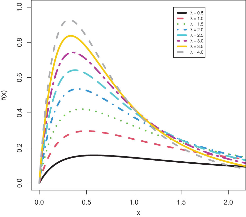
Different shapes of the PDF for the ITL distribution.

Figure 2

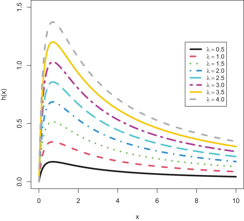
Different shapes of the HRF for the ITL distribution.

2.2 Basic assumptions

All items are randomly allocated to two samples of size n ( 1 − τ ) and n τ , respectively, where τ is the sample proportion. The first sample is assigned to usual conditions, while the second is assigned to accelerated conditions. Each test item in each sample is performed without modifying the test condition until the censoring number is obtained.

Assumptions:

The lifetimes X i ; i = 1 , … , n ( 1 − τ ) of units assigned to usual conditions are independent and identically distributed (i.i.d) random variables.
The lifetimes Y j ; j = 1 , … , n τ of units assigned to accelerated conditions are i.i.d random variables.
The lifetimes X i and Y j are mutually statistically independent.

Assuming that lifetimes of test items have the ITL distribution, then the PDF of an item at usual conditions is defined in equation (4). For an item tested under accelerated conditions, the PDF and CDF are derived as follows:

(8) f ( y ; λ , β ) = 2 λ β y ( 1 + β y ) − 2 λ − 1 ( 1 + 2 β y ) λ − 1 , y > 0 ; λ > 0 , β > 1 ,

and

(9) F ( y ; λ , β ) = 1 − ( 1 + 2 β y ) λ ( 1 + β y ) 2 λ , y > 0 ; λ > 0 , β > 1 ,

where Y = β − 1 X , β is the acceleration factor defined as the ratio of the mean life under usual conditions to that under accelerated conditions, and β > 1 .

For an item tested under accelerated conditions, the RF and HRF are provided as follows:

(10) R ( y ; λ , β ) = ( 1 + 2 β y ) λ ( 1 + β y ) 2 λ , y > 0 ; λ > 0 , β > 1 ,

and

(11) h ( y ; λ , β ) = 2 λ β y [ ( 1 + β y ) ( 1 + 2 β y ) ] − 1 , y > 0 ; λ > 0 , β > 1 .

3 Bayesian estimation

Based on CS-PALT using Type-II censored samples, the Bayes estimators for the unknown parameter and the acceleration factor of the ITL distribution are presented in this section.

Let us consider that the periods of failure contain the r th smallest lifetimes x ( 1 ) ⩽ x ( 2 ) ⩽ … ⩽ x ( r ) from a random sample of n ( 1 − τ ) based on usual conditions and y ( 1 ) ⩽ y ( 2 ) ⩽ … ⩽ y ( r ) from a random sample of n τ at accelerated conditions, respectively.

Under usual conditions, the likelihood function (LF) of x ( i ) ; i = 1 , … , n ( 1 − τ ) is as follows:

(12) L u ( λ ∣ x ̲ ) ∝ ∏ i = 1 r f ( x ( i ) ∣ λ ) [ R ( x ( r ) ∣ λ ) ] n ( 1 − τ ) − r ,

where x ̲ = x ( 1 ) , x ( 2 ) , … , x [ n ( 1 − τ ) − r ] , and f ( x ( i ) ∣ λ ) , and R ( x ( r ) ∣ λ ) are given by Eqs. (4) and (6), respectively. The LF for y ( j ) , j = 1 , … , n τ , at accelerated conditions is defined as follows:

(13) L a ( θ ̲ ∣ y ̲ ) ∝ ∏ j = 1 r f ( y ( j ) ∣ θ ̲ ) [ R ( y ( r ) ∣ θ ̲ ) ] n τ − r ,

where y ̲ = y ( 1 ) , y ( 2 ) , … , y ( n τ − r ) , θ ̲ = ( λ , β ) ′ , and f ( y ( j ) ∣ θ ̲ ) , R ( y ( r ) ∣ θ ̲ ) are given by Eqs. (8) and (10), respectively.

Assuming that m u and m a represent the number of units that are censored under usual and accelerated conditions, where

(14) m u = n ( 1 − τ ) − r and m a = n τ − r ,

where r is the censoring level and is assumed to be equal under usual and accelerated conditions.

Substituting Eqs. (4) and (6) into Eq. (12) and substituting Eqs. (8) and (10) into Eq. (13), hence the LF according to CS-PALT for x ( i ) and y ( j ) , where i = 1 , … , n ( 1 − τ ) and j = 1 , … , n τ , can be expressed as follows:

(15) L ( θ ̲ ∣ x , ̲ y ̲ ) ∝ ( 2 λ ) 2 r β r ∏ i = 1 r x ( i ) ( 1 + x ( i ) ) − 2 λ − 1 × ( 1 + 2 x ( i ) ) λ − 1 ( 1 + 2 x ( r ) ) λ ( 1 + x ( r ) ) 2 λ m u × ∏ j = 1 r y ( j ) ( 1 + β y ( j ) ) − 2 λ − 1 ( 1 + 2 β y ( j ) ) λ − 1 × ( 1 + 2 β y ( r ) ) λ ( 1 + β y ( r ) ) 2 λ m a .

The natural logarithm of LF in Eq. (15) is given as follows:

(16) ℓ ∝ 2 r log ( λ ) + r log ( β ) − ( 2 λ + 1 ) ∑ i = 1 r log [ 1 + x ( i ) ] + ∑ i = 1 r log [ x ( i ) ] + ( λ − 1 ) ∑ i = 1 r log [ 1 + 2 x ( i ) ] + m u log ( 1 + 2 x ( r ) ) λ ( 1 + x ( r ) ) 2 λ + ∑ j = 1 r log [ y ( j ) ] − ( 2 λ + 1 ) ∑ j = 1 r log [ 1 + β y ( j ) ] + ( λ − 1 ) ∑ j = 1 r log [ 1 + 2 β y ( j ) ] + m a log ( 1 + 2 β y ( r ) ) λ ( 1 + β y ( r ) ) 2 λ .

By differentiating Eq. (16) with regard to λ and β and then setting to zero, the ML estimators of the unknown parameter and the acceleration factor, θ ̲ = ( λ , β ) ′ , can be derived as follows:

(17) ∂ ℓ ∂ λ = 2 r λ − 2 ∑ i = 1 r log [ 1 + x ( i ) ] + ∑ i = 1 r log [ 1 + 2 x ( i ) ] + m u log ( 1 + 2 x ( r ) ) ( 1 + x ( r ) ) 2 − 2 ∑ j = 1 r log [ 1 + β y ( j ) ] + ∑ j = 1 r log [ 1 + 2 β y ( j ) ] + m a log ( 1 + 2 β y ( r ) ) ( 1 + β y ( r ) ) 2 ,

and

(18) ∂ ℓ ∂ β = r β − ( 2 λ + 1 ) ∑ j = 1 r y ( j ) ( 1 + β y ( j ) ) + ( λ − 1 ) ∑ j = 1 r 2 y ( j ) ( 1 + 2 β y ( j ) ) − 2 λ β m a y ( r ) 2 ( 1 + β y ( r ) ) ( 1 + 2 β y ( r ) ) .

By equating the derivatives (17) and (18) to zeros, the ML estimators for the unknown parameters λ and β are produced. The ML estimates for the unknown parameters λ and β can be obtained by numerically solving the system of nonlinear equations using the Newton–Raphson method.

Regarding the pre-existing knowledge pertaining to the vector of parameters θ ̲ = ( λ , β ) ′ , is correctly characterized by an informative prior that is a gamma distribution with parameters a j and b j and PDF as below:

(19) π ( θ j ; a j , b j ) = b j a j Γ ( a j ) θ j a j − 1 exp ( − b j θ j ) , θ j , a j , b j > 0 ; j = 1 , 2 , … ,

where, θ 1 = λ and θ 2 = β , and a j and b j are the hyper-parameters of the prior distribution.

Supposing that the parameters, θ ̲ = ( λ , β ) ′ , are independent and unknown, then the joint prior distribution for the unknown parameters has a joint PDF defined as follows:

(20) π ( θ ̲ ; a ̲ , b ̲ ) ∝ λ a 1 − 1 β a 2 − 1 exp [ − ( b 1 λ + b 2 β ) ] ,

where λ > 0 and β > 1 , and ( a ̲ , b ̲ > 0 ̲ ) . The joint posterior distribution of the parameters, θ ̲ = ( λ , β ) ′ , may be computed by inserting the LF in Eq. (15), and the joint prior distribution provided by Eq. (20) is given as follows:

(21) π ( θ ̲ ∣ x ̲ , y ̲ ) ∝ L ( θ ̲ ∣ x , ̲ y ̲ ) π ( θ ̲ ; a ̲ , b ̲ ) ∝ λ 2 r + a 1 − 1 β r + a 2 − 1 exp [ − ( b 1 λ + b 2 β ) ] × ∏ i = 1 r ( 1 + x ( i ) ) − 2 λ ( 1 + 2 x ( i ) ) λ × ∏ j = 1 r ( 1 + β y ( j ) ) − 2 λ − 1 ( 1 + 2 β y ( j ) ) λ − 1 × ( 1 + 2 x ( r ) ) λ ( 1 + x ( r ) ) 2 λ m u ( 1 + 2 β y ( r ) ) λ ( 1 + β y ( r ) ) 2 λ m a .

The joint posterior distribution provided by Eq. (21) may be expressed as follows:

(22) π ( θ ̲ ∣ x ̲ , y ̲ ) = A λ 2 r + a 1 − 1 β r + a 2 − 1 exp [ − ( b 1 λ + b 2 β ) ] × ∏ i = 1 r ( 1 + x ( i ) ) − 2 λ ( 1 + 2 x ( i ) ) λ × ∏ j = 1 r ( 1 + β y ( j ) ) − 2 λ − 1 ( 1 + 2 β y ( j ) ) λ − 1 × ( 1 + 2 x ( r ) ) λ ( 1 + x ( r ) ) 2 λ m u ( 1 + 2 β y ( r ) ) λ ( 1 + β y ( r ) ) 2 λ m a ,

where

(23) A − 1 = ∫ θ ̲ λ 2 r + a 1 − 1 β r + a 2 − 1 exp [ − ( b 1 λ + b 2 β ) ] × ∏ i = 1 r ( 1 + x ( i ) ) − 2 λ ( 1 + 2 x ( i ) ) λ × ∏ j = 1 r ( 1 + β y ( j ) ) − 2 λ − 1 ( 1 + 2 β y ( j ) ) λ − 1 × ( 1 + 2 x ( r ) ) λ ( 1 + x ( r ) ) 2 λ m u ( 1 + 2 β y ( r ) ) λ ( 1 + β y ( r ) ) 2 λ m a d θ ̲ ,

and

(24) ∫ θ ̲ = ∫ λ ∫ β and d θ ̲ = d β d λ .

The Bayes estimators are derived using two different loss functions, the BSEL and BLL functions, which are symmetric and asymmetric loss functions.

3.1 Bayes estimators under BSEL function

Using Eqs. (2) and (22), the Bayes estimators for the parameters using the BSEL function may be derived as follows:

(25) θ ˜ jBSE = ω θ ˆ jML + ( 1 − ω ) ∫ θ ̲ θ j π ( θ ̲ ∣ x ̲ , y ̲ ) d θ ̲ = ω θ ˆ jML + ( 1 − ω ) A ∫ θ ̲ θ j λ 2 r + a 1 − 1 β r + a 2 − 1 × ( 1 + 2 x ( r ) ) λ ( 1 + x ( r ) ) 2 λ m u ( 1 + 2 β y ( r ) ) λ ( 1 + β y ( r ) ) 2 λ m a × exp [ − ( b 1 λ + b 2 β ) ] ∏ i = 1 r ( 1 + x ( i ) ) − 2 λ ( 1 + 2 x ( i ) ) λ × ∏ j = 1 r ( 1 + β y ( j ) ) − 2 λ − 1 ( 1 + 2 β y ( j ) ) λ − 1 d θ ̲ ,

where θ 1 = λ and θ 2 = β , θ ˆ M L is the estimator of θ j using the ML approach depending on Eqs. (17) and (18), A − 1 is defined in Eq. (23), and ∫ θ ̲ and d θ ̲ are given in Eq. (24).

3.2 Bayes estimators under BLL function

From Eqs. (3) and (22), the Bayes estimators of the parameters using the BLL function may be calculated as follows:

(26) θ ˜ jBLL = − 1 v ln ω exp ( − v θ ˆ jML ) + ( 1 − ω ) ∫ θ ̲ exp ( − v θ j ) π ( θ ̲ ∣ x ̲ , y ̲ ) d θ ̲ = − 1 v ln ω exp ( − v θ ˆ M L ) + ( 1 − ω ) A ∫ θ ̲ λ 2 r + a 1 − 1 β r + a 2 − 1 × exp [ − ( v θ j + b 1 λ + b 2 β ) ] ∏ i = 1 r ( 1 + x ( i ) ) − 2 λ ( 1 + 2 x ( i ) ) λ × ∏ j = 1 r ( 1 + β y ( j ) ) − 2 λ − 1 ( 1 + 2 β y ( j ) ) λ − 1 × ( 1 + 2 x ( r ) ) λ ( 1 + x ( r ) ) 2 λ m u ( 1 + 2 β y ( r ) ) λ ( 1 + β y ( r ) ) 2 λ m a d θ ̲ .

The Bayes estimators for the unknown parameters, θ ̲ = ( λ , β ) ′ , using BLL function may be computed by substituting θ j by λ or β in Eq. (26).

4 E-Bayesian estimation

The E-Bayes estimators of the parameters, θ ̲ = ( λ , β ) ′ , for the ITL distribution under CS-PALT using a Type-II censored sample are obtained in this section.

Han [13] indicated that the hyper-parameters a j and b j must be chosen to ensure that π ( θ j ; a j , b j ) , provided in Eq. (19), can be decreasing functions of θ j ( j = 1 , 2 ).

The derivative of π ( θ j ; a j , b j ) with regard to θ j is shown below:

(27) d π ( θ j ; a j , b j ) d θ j = b j a j Γ ( a j ) θ j a j − 2 × exp ( − b j θ j ) ( a j − 1 − b j θ j ) , j = 1 , 2 ,

for 0 < a j < 1 and b j > 0 , then d π ( θ j ; a j , b j ) d θ j < 0 , which means that π ( θ j ; a j , b j ) can be decreasing functions of θ j .

To derive the E-Bayes estimators of the parameters, three alternative distributions for the hyper-parameters a j and b j are employed. These distributions are used to determine how different prior distributions affect the E-Bayes estimator for θ j .

Given the assumption of independence of hyper-parameters a j and b j it may be inferred that they possess bivariate density functions

(28) π ℏ ( a j , b j ) = π ℏ ( a j ) π ℏ ( b j ) , j = 1 , 2 , ℏ = 1 , 2 , … , 6 .

Then, the bivariate uniform hyperprior distributions are given as follows:

(29) π ℏ ( a j , b j ) = 2 ( c j − b j ) c j 2 , 0 < a j < 1 , 0 < b j < c j ,

(30) π ℏ ( a j , b j ) = 1 c j , 0 < a j < 1 , 0 < b j < c j ,

(31) π ℏ ( a j , b j ) = 2 b j c j 2 , 0 < a j < 1 , 0 < b j < c j .

The E-Bayes estimators of θ j (expectation of the Bayes estimators of θ j ) may be derived as follows:

(32) θ ˜ j E B = E π ℏ ( θ ˜ j B ( a j , b j ) ) = ∬ D θ ˜ j B ( a j , b j ) π ℏ ( a j , b j ) d a j d b j j = 1 , 2 , ℏ = 1 , 2 , … , 6 ,

where E π ℏ ( ℏ = 1 , 2 , … , 6 ) represents the expected value of the bivariate hyperprior distributions, D is the domain of the function π ℏ ( a j , b j ) , and θ ˜ j B ( a j , b j ) are the Bayes estimators for the parameters θ j under BSEL and BLL functions.

The E-Bayes estimators are derived using two different loss functions, the BSEL and BLL functions, which are symmetric and asymmetric loss functions.

4.1 E-Bayes estimators under BSEL function

The three E-Bayes estimators of the parameter θ j using BSEL function may be computed by substituting Eqs. (25) and (29)–(31) in Eq. (32) as, respectively, as follows:

(33) θ ˜ j EBBS 1 = 2 c j 2 ∫ 0 1 ∫ 0 c j [ ω θ ^ j M L + ( 1 − ω ) A × ∫ θ ̲ θ j λ 2 r + a 1 − 1 β r + a 2 − 1 e − ( b 1 λ + b 2 β ) × ∏ i = 1 r ( 1 + x ( i ) ) − 2 λ ( 1 + 2 x ( i ) ) λ × ( 1 + 2 x ( r ) ) λ ( 1 + x ( r ) ) 2 λ m u ( 1 + 2 β y ( r ) ) λ ( 1 + β y ( r ) ) 2 λ m a × [ ∏ j = 1 ( 1 + β y ( j ) ) − 2 λ − 1 ( 1 + 2 β y ( j ) ) λ − 1 ] d θ ̲ ] ( c j − b j ) d a j d b j .

(34) θ ˜ j EBBS 2 = 1 c j ∫ 0 1 ∫ 0 c j [ ω θ ^ j M L + ( 1 − ω ) A × ∫ θ ̲ θ j λ 2 r + a 1 − 1 β r + a 2 − 1 exp [ − ( b 1 λ + b 2 β ) ] × ∏ i = 1 r ( 1 + x ( i ) ) − 2 λ ( 1 + 2 x ( i ) ) λ × ( 1 + 2 x ( r ) ) λ ( 1 + x ( r ) ) 2 λ m u × ( 1 + 2 β y ( r ) ) λ ( 1 + β y ( r ) ) 2 λ m a × ∏ j = 1 r ( 1 + β y ( j ) ) − 2 λ − 1 ( 1 + 2 β y ( j ) ) λ − 1 d θ ̲ d a j d b j .

and

(35) θ ˜ j EBBS 3 = 2 c j 2 ∫ 0 1 ∫ 0 c j [ ω θ ^ j M L + ( 1 − ω ) A × ∫ θ ̲ θ j λ 2 r + a 1 − 1 β r + a 2 − 1 exp [ − ( b 1 λ + b 2 β ) ] × ∏ i = 1 r ( 1 + x ( i ) ) − 2 λ ( 1 + 2 x ( i ) ) λ × ( 1 + 2 x ( r ) ) λ ( 1 + x ( r ) ) 2 λ m u × ( 1 + 2 β y ( r ) ) λ ( 1 + β y ( r ) ) 2 λ m a × ∏ j = 1 r ( 1 + β y ( j ) ) − 2 λ − 1 ( 1 + 2 β y ( j ) ) λ − 1 d θ ̲ ( b j ) d a j d b j ,

where j = 1 , 2 , θ 1 = λ , θ 2 = β , θ ^ j M L is the estimator of θ j using the ML approach depending on Eqs. (17) and (18), A − 1 is defined as in Eq. (23), and ∫ θ ̲ and d θ ̲ are given in Eq. (24).

One can calculate the three E-Bayes estimators of the parameters, θ ̲ = ( λ , β ) ′ , under BSEL function by substituting j by 1 or 2 in (33)–(35).

4.2 E-Bayes estimators under BLL function

Substituting Eqs. (26) and (29)–(31) in Eq. (32), the three E-Bayes estimators for the parameter θ j using BLL function are computed as follows:

(36) θ ˜ jEBBL1 = 2 c j 2 ∫ 0 1 ∫ 0 c j − 1 v ln [ ω exp ( − v θ ^ j ML ) + ( 1 − ω ) A ∫ θ ̲ λ 2 r + a 1 − 1 β r + a 2 − 1 exp [ − ( b 1 λ + b 2 β ) ] × ∏ i = 1 r ( 1 + x ( i ) ) − 2 λ ( 1 + 2 x ( i ) ) λ × ( 1 + 2 x ( r ) ) λ ( 1 + x ( r ) ) 2 λ m u × [ ∏ j = 1 ( 1 + β y ( j ) ) − 2 λ − 1 ( 1 + 2 β y ( j ) ) λ − 1 ] × ( 1 + 2 β y ( r ) ) λ ( 1 + β y ( r ) ) 2 λ m a d θ ̲ ( c j − b j ) d a j d b j ,

(37) θ ˜ jEBBL2 = 1 c j ∫ 0 1 ∫ 0 c j − 1 v ln [ ω exp ( − v θ ^ j ML ) + ( 1 − ω ) A ∫ θ ̲ λ 2 r + a 1 − 1 β r + a 2 − 1 exp [ − ( v θ j + b 1 λ + b 2 β ) ] × ∏ i = 1 r ( 1 + x ( i ) ) − 2 λ ( 1 + 2 x ( i ) ) λ × ( 1 + 2 x ( r ) ) λ ( 1 + x ( r ) ) 2 λ m u × [ ∏ j = 1 ( 1 + β y ( j ) ) − 2 λ − 1 ( 1 + 2 β y ( j ) ) λ − 1 ] × ( 1 + 2 β y ( r ) ) λ ( 1 + β y ( r ) ) 2 λ m a d θ ̲ d a j d b j ,

and

(38) θ ˜ j EBBL3 = 2 c j 2 ∫ 0 1 ∫ 0 c j − 1 v ln [ { ω exp ( − v θ ^ j ML ) + ( 1 − ω ) A ∫ θ ̲ λ 2 r + a 1 − 1 β r + a 2 − 1 exp [ − ( v θ j + b 1 λ + b 2 β ) ] × ∏ i = 1 r ( 1 + x ( i ) ) − 2 λ ( 1 + 2 x ( i ) ) λ × ( 1 + 2 x ( r ) ) λ ( 1 + x ( r ) ) 2 λ m u × ( ∏ j = 1 ( 1 + β y ( j ) ) − 2 λ − 1 ( 1 + 2 β y ( j ) ) λ − 1 ) × ( 1 + 2 β y ( r ) ) λ ( 1 + β y ( r ) ) 2 λ m a d θ ̲ ( b j ) d a j d b j .

One may compute the three E-Bayes estimators of the parameters, θ ̲ = ( λ , β ) ′ , using BLL function by substituting j by 1 or 2 in Eqs. (36)–(38).

5 Numerical illustration

In this section, the accuracy of theoretical results of Bayes and E-Bayes estimates are investigated using simulated and real datasets.

5.1 Simulation algorithm

A simulation study is carried out in this subsection to demonstrate the efficiency of the provided Bayes and E-Bayes estimates for CS-PALT using Type-II censored data generated from the ITL distribution. For all simulation investigations, the R programming language is used.

The following are the steps of the simulation process using Type-II censored data:

Random samples of size n are generated from the ITL ( λ ) distribution for specified values of λ .
1. Hassan et al. [20] provided the following transformation between the uniform distribution and the ITL ( λ ) distribution:
  x u = − ( 1 − u ) 1 λ − 1 ( 1 − u ) 1 λ + ( 1 − u ) 1 λ − 1 2 − ( 1 − u ) 1 λ ( 1 − u ) 1 λ − 1 ( 1 − u ) 1 λ ,
  where u ∈ ( 0 , 1 ) .
Generate a j and b j from the bivariate uniform hyperprior distributions, π ℏ ( a j , b j ) , j = 1 , 2 , ℏ = 1 , 2 , … , 6 , as given in Eqs. (29)–(31).
For given values of a j and b j , generate λ and β from the gamma prior distributions.
For each sample size, the values of x i are sorted where x ( 1 ) ⩽ x ( 2 ) ⩽ … ⩽ x [ n ( 1 − τ ) ] .
For each sample size, the values of y i are sorted as y ( 1 ) ⩽ y ( 2 ) ⩽ … ⩽ y ( n τ ) .
Considering two different proportions τ for the sample units assigned to accelerated conditions τ = 20% and τ = 50% under Type-II censored data.
The number of failures r is chosen to be less than n ( 1 − τ ) and n τ .
Calculate the Bayes and E-Bayes estimates for the parameters using the BSEL and BLL functions.
Repeat all the previous steps N = 10,000 times for the samples of size n = 20 , 60, and 100.

The accuracy of the estimates is used to evaluate their performance. It is convenient to use the estimated risk (ER) = ∑ i = 1 N ( estimated value − true value ) 2 N to investigate the precision and variation of the estimates.

Tables A1, A2, A3, A4, A5, A6 display the Bayes and E-Bayes averages and ERs of the unknown parameter and the acceleration factor of the ITL distribution for CS-PALT under BSEL and BLL functions using Type-II censored data, where the censoring level is 10% n for each sample size, the sample proportions are 0.20 and 0.50, and the specified values of parameters are (Case 1: λ = 0.5 and β = 1.5), (Case 2: λ = 0.5 and β = 2.5), and (Case 3: λ = 0.5 and β = 3.5). Tables A7 and A8 display the Bayes and E-Bayes averages and expected risks (ERs) for the unknown parameters under BSEL and BLL functions based on Type-II censoring for different weights ω ; ω = 0 , 0.3, 0.6 and 1 where when ω = 0, the Bayes estimates using the BSEL or BLL functions are obtained and when ω = 1, the ML estimates are obtained.

5.2 Real datasets

The major objective of this subsection is to show how the recommended methods can be applied in practice. This is achieved using two real-life datasets. To demonstrate that the ITL distribution is fitted to the two real datasets, the Kolmogorov–Smirnov goodness-of-fit test is applied in the R programming language.

Data 1

The first data are presented by Liu et al. [21]. The data correspond to the survival times of patients in China affected by the COVID-19 pandemic. The dataset under consideration represents the survival periods of patients from the moment they were admitted to the hospital untill death. From January through February 2020, 53 COVID-19 patients were identified at the hospital in serious condition. The dataset is presented as follows: 20.083, 6.743, 0.064, 10.827, 0.087, 0.976, 16.978, 0.364, 4.237, 1.756, 0.816, 4.190, 0.704, 5.028, 19.092, 0.421, 7.274, 0.796, 0.479, 3.867, 14.278, 0.568, 8.273, 3.890, 0.865, 17.209, 3.543, 0.235, 15.287, 2.869, 0.054, 13.324, 0.352, 6.174, 0.787, 0.087, 9.324, 0.458, 11.282, 0.437, 7.058, 0.978, 0.976, 5.083, 0.548, 4.092, 1.978, 4.093, 3.079, 2.089, 3.646, 3.348 and 2.643, see, https://www.worldometers.info/coronavirus/.

Data 2

The second dataset is a 59-day COVID-19 mortality rate dataset from Italy, collected from 27 February 2020 through 27 April 2020 and given by Almongy et al. [22]. The dataset is as follows: 4.571, 7.201, 3.606, 8.479, 11.410, 8.961, 10.919, 10.908, 6.503, 18.474, 11.010, 17.337, 16.561, 13.226, 15.137, 8.697, 15.787, 13.333, 11.822, 14.242, 11.273, 14.330, 16.046, 11.950, 10.282, 11.775, 10.138, 9.037, 12.396, 10.644, 8.646, 8.905, 8.906, 7.407, 7.445, 7.214, 6.194, 4.640, 5.452, 5.073, 4.416, 4.859, 4.408, 4.639, 3.148, 4.040, 4.253, 4.011, 3.564, 3.827, 3.134, 2.780, 2.881, 3.341, 2.686, 2.814, 2.508, 2.450, and 1.518 (see https://covid19.who.int/). The validity of the fitted model is checked through the Kolmogorov–Smirnov goodness-of-fit test. The p -values are 0.7444 and 0.2582, respectively. In each case, the p -value indicated that the model suited the data. The Bayes and E-Bayes estimates and standard errors (SEs) of the unknown parameters for the real datasets using BSEL and BLL functions are presented in Tables A9 and A10.

5.3 Concluding remarks

According to Tables A1–A6, as the sample size increases, the accuracy of the ER improves.
When the acceleration factor β increases, the ERs decrease, as shown in Tables A1–A6.
Tables A1 and A2 demonstrate that the ERs of the parameters perform better as the proportion τ of the sample units assigned to accelerated conditions decreases.
The E-Bayes estimators consistently outperform the Bayes estimators because the ERs of the E-Bayes estimates of the parameters are always lower than the ERs of the Bayes estimates, as in Tables A1–A8.
From Tables A1–A8, the Bayes and E-Bayes estimators using the BLL function usually perform better than the Bayes and E-Bayes estimators using the BSEL function, as demonstrated by the fact that the ERs of Bayes and E-Bayes estimates using the BLL function, are lower than the ERs of Bayes and E-Bayes estimates using the BSEL function.
Tables A7 and A8 show that the Bayes estimates using the BSEL or BLL functions are obtained when ω = 0 and the ML estimates are obtained when ω = 1 .

6 General conclusion

The measurement of product life using usual conditions frequently demands a lengthy period of time for products with a high level of reliability. Thus, ALT or PALT is employed to make it easier to estimate the unit’s reliability rapidly. Because ALT items are only processed under accelerated conditions, such relationships cannot be known or presumed in some cases. As a result, PALT is frequently employed in such cases; in PALT, items are performed under both usual and accelerated conditions. Based on Type-II censoring, this study presented a CS-PALT. A CS-PALT includes performing each test item under usual or accelerated conditions under constant stress until the test is completed. Considering that the lifetimes of test products have the ITL distribution. The distribution parameter and the acceleration factor of the ITL distribution are estimated using the Bayesian and E-Bayesian methods. The estimators are obtained using two different loss functions, the BSEL and BLL functions, which are symmetric and asymmetric loss functions. The BLF is a mixture of Bayes and non-Bayes estimators. The performance of the proposed Bayes and E-Bayes estimates is evaluated through a simulation study and an application using real datasets. In general, numerical computations showed that as the sample size increases and the weight ω decreases, the accuracy of the ER improves. In addition, the ERs of the parameters decrease when the acceleration factor increases and the proportion sample ( τ ) decreases. The E-Bayes estimators consistently outperform the Bayes estimators because the ERs of the E-Bayes estimates of the parameters are always lower than the ERs of the Bayes estimates. The E-Bayesian and Bayesian methods for estimating the parameters of the ITL distribution for CS-PALT using different types of loss functions, such as general entropy and precautionary loss functions, would be useful as a basis for future distribution theory research.

Acknowledgments

The authors acknowledge Princess Nourah bint Abdulrahman University Researchers Supporting Project number (PNURSP2023R368), Princess Nourah bint Abdulrahman University, Riyadh, Saudi Arabia.

Funding information: Princess Nourah bint Abdulrahman University Researchers Supporting Project number (PNURSP2023R368), Princess Nourah bint Abdulrahman University, Riyadh, Saudi Arabia.
Author contributions: All authors have accepted responsibility for the entire content of this manuscript and approved its submission.
Conflict of interest: The authors state no conflict of interest.
Data availability statement: All data generated or analysed during this study are included in this published article [and its supplementary information files].

Appendix 1

Table A1

The averages and ERs of the parameters under BSEL function using Type-II censoring (Case 1: N = 10,000 , τ = 0.20 , 0.50, r = 0.1 n , ω = 0.3 , λ = 0.5 , and β = 1.5 )

n	r	τ	θ ̲	Averages		ERs
				θ ̲ ˜ B	θ ̲ ˜ E B	θ ̲ ˜ B	θ ̲ ˜ E B
20	2	0.2	λ	0.4711	0.4859	0.0014	0.0008
					0.4971		0.0011
					0.4777		0.0002
			β	1.3748	1.4084	0.0187	0.0023
					1.3775		0.002
					1.4363		0.0052
			λ	0.5573	0.5277	0.0108	0.0018
					0.5713		0.0019
					0.5627		0.0017
		0.5	β	1.2298	1.2115	0.0304	0.0027
					1.2322		0.0021
					1.1008		0.0183
60	6	0.2	λ	0.53	0.5302	0.0013	9.5472 × 1 0 ‒ 5
					0.5135		4.1418 × 1 0 ‒ 4
					0.5367		2.4292 × 1 0 ‒ 4
			β	1.4945	1.4862	0.0004	1.7235 × 1 0 ‒ 4
					1.5083		3.8464 × 1 0 ‒ 4
					1.4958		2.8165 × 1 0 ‒ 4
		0.5	λ	0.4477	0.4814	0.0039	0.0014
					0.4801		0.0012
					0.415		0.0014
			β	1.4838	1.463	0.001	0.0006
					1.496		0.0004
					1.4645		0.0008
100	10	0.2	λ	0.4818	0.4791	0.0006	1.7787 × 1 0 ‒ 5
					0.4765		3.4436 × 1 0 ‒ 5
					0.4895		7.7972 × 1 0 ‒ 5
			β	1.4884	1.4776	0.0002	1.3484 × 1 0 ‒ 4
					1.49		9.8486 × 1 0 ‒ 6
					1.4885		1.7907 × 1 0 ‒ 5
		0.5	λ	0.4737	0.4943	0.0012	5.1975 × 1 0 ‒ 4
					0.4469		9.0124 × 1 0 ‒ 4
					0.4638		2.1239 × 1 0 ‒ 4
			β	1.5157	1.518	0.0004	3.0119 × 1 0 ‒ 4
					1.5119		9.4147 × 1 0 ‒ 5
					1.4984		3.4475 × 1 0 ‒ 4

Table A2

The averages and ERs of the parameters under BLL function using Type-II censoring (Case 1: N = 10,000 , τ = 0.20 , 0.50, r = 0.1 n , ω = 0.3 , v = ‒ 2 , λ = 0.5 and β = 1.5 )

n	r	τ	θ ̲	Averages		ERs
				θ ̲ ˜ B	θ ̲ ˜ E B	θ ̲ ˜ B	θ ̲ ˜ E B
20	2	0.2	λ	0.4586	0.4438		0.0005
					0.4423	0.0021	0.0011
					0.4451		0.0017
			β	1.4589	1.4381		0.001
					1.4412	0.0021	0.0006
					1.446		0.0008
		0.5	λ	0.5382	0.5939		0.0036
					0.5063	0.0037	0.0018
					0.5864		0.003
			β	1.0112	0.9478		0.0055
					1.0352	0.0096	0.0015
					0.9496		0.0052
60	6	0.2	λ	0.5254	0.5253		4.98 × 1 0 ‒ 5
					0.5437	0.0012	5.02 × 1 0 ‒ 4
					0.5197		2.28 × 1 0 ‒ 4
			β	1.4917	1.4889		4.24 × 1 0 ‒ 5
					1.5028	0.0003	2.15 × 1 0 ‒ 4
					1.5007		1.61 × 1 0 ‒ 4
		0.5	λ		0.5163		0.0007
				0.5325	0.5458	0.0027	0.0009
					0.5149		0.0013
			β		1.4828		0.0007
				1.4612	1.4742	0.0028	0.0004
					1.4336		0.0009
100	10	0.2	λ		0.4826		1.41 × 1 0 ‒ 5
				0.4824	0.477	0.0004	4.14 × 1 0 ‒ 5
					0.4855		1.65 × 1 0 ‒ 5
			β		1.4922		8.86 × 1 0 ‒ 6
				1.4936	1.4913	0.0001	1.75 × 1 0 ‒ 5
					1.495		1.78 × 1 0 ‒ 5
		0.5	λ		0.4639		2.75 × 1 0 ‒ 4
				0.4759	0.4715	0.0006	1.74 × 1 0 ‒ 4
					0.4966		4.85 × 1 0 ‒ 4
			β		1.4607		7.86 × 1 0 ‒ 5
				1.46	1.4688	0.0018	1.26 × 1 0 ‒ 4
					1.4567		1.80 × 1 0 ‒ 4

Table A3

The averages and ERs of the parameters under BSEL function using Type-II censoring (Case 2: N = 10,000 , τ = 0.50 , r = 0.1 n , ω = 0.3 , λ = 0.5 , and β = 2.5 )

n	r	τ	θ ̲	Averages		ERs
				θ ̲ ˜ B	θ ̲ ˜ E B	θ ̲ ˜ B	θ ̲ ˜ E B
			λ		0.5671		0.0012
20	2	0.5		0.5515	0.5662	0.0032	0.0007
					0.5438		0.0003
			β		2.5922		0.0005
				2.5855	2.556	0.0095	0.002
					2.5499		0.0021
			λ		0.5214		0.0004
				0.5158	0.532	0.0008	0.0007
60	6	0.5			0.5163		0.0002
			β		2.4649		0.0004
				2.476	2.4634	0.0009	0.0002
					2.4634		0.0002
			λ		0.5219		5.78 × 1 0 ‒ 5
				0.5218	0.5134	0.0007	1.02 × 1 0 ‒ 4
100	10	0.5			0.5228		4.92 × 1 0 ‒ 5
			β		2.4975		7.24 × 1 0 ‒ 5
				2.4933	2.4909	0.0002	8.24 × 1 0 ‒ 5
					2.5024		1.26 × 1 0 ‒ 4

Table A4

The averages and ERs of the parameters under BLL function using Type-II censoring (Case 2: N = 10,000 , τ = 0.50 , r = 0.1 n , ω = 0.3 , v = ‒ 2 , λ = 0.5 , β = 2.5 )

n	r	τ	θ ̲	Averages		ERs
				θ ̲ ˜ B	θ ̲ ˜ E B	θ ̲ ˜ B	θ ̲ ˜ E B
20	2	0.5	λ	0.5284	0.5094		0.0006
					0.5086	0.0019	0.0009
					0.4873		0.0018
			β	2.4177	2.4441		0.0009
					2.4307	0.0083	0.0003
					2.3968		0.0007
60	6	0.5	λ	0.5185	0.5283		1.54 × 1 0 ‒ 4
					0.5206	0.0006	2.09 × 1 0 ‒ 5
					0.5322		3.82 × 1 0 ‒ 4
			β	2.4795	2.4682		1.84 × 1 0 ‒ 4
					2.4889	0.0008	2.04 × 1 0 ‒ 4
					2.4659		2.78 × 1 0 ‒ 4
100	10	0.5	λ	0.5115	0.5059		4.52 × 1 0 ‒ 5
					0.5092	0.0004	1.36 × 1 0 ‒ 5
					0.5135		9.74 × 1 0 ‒ 5
			β	2.4903	2.4953		3.96 × 1 0 ‒ 5
					2.4848	0.0002	4.75 × 1 0 ‒ 5
					2.4931		2.72 × 1 0 ‒ 5

Table A5

The averages and ERs of the parameters under BSEL function using Type-II censoring (Case 3: N = 10,000 , τ = 0.50 , r = 0.1 n , ω = 0.3 , λ = 0.5 , and β = 3.5 )

n	r	τ	θ ̲	Averages		ERs
				θ ̲ ˜ B	θ ̲ ˜ E B	θ ̲ ˜ B	θ ̲ ˜ E B
20	2	0.5	λ	0.5474	0.5247	0.0031	0.0007
					0.5317		0.0005
					0.5343		0.0002
			β	3.4595	3.442	0.0023	0.0004
					3.4221		0.0018
					3.4722		0.0003
60	6	0.5	λ	0.5181	0.5108	0.0007	1.15 × 1 0 ‒ 4
					0.5337		2.98 × 1 0 ‒ 4
					0.5128		7.60 × 1 0 ‒ 5
			β	3.5105	3.5116	0.0004	6.22 × 1 0 ‒ 5
					3.5224		1.72 × 1 0 ‒ 4
					3.5142		7.54 × 1 0 ‒ 5
100	10	0.5	λ	0.483	0.4772	0.0005	4.87 × 1 0 ‒ 5
					0.4857		2.53 × 1 0 ‒ 5
					0.4849		1.92 × 1 0 ‒ 5
			β	3.5081	3.5139	0.0001	5.54 × 1 0 ‒ 5
					3.5135		6.63 × 1 0 ‒ 5
					3.5051		2.56 × 1 0 ‒ 5

Table A6

The averages and ERs of the parameters under BLL function using Type-II censoring (Case 3: N = 10,000 , τ = 0.50 , r = 0.1 n , ω = 0.3 , v = ‒ 2 , λ = 0.5 , and β = 3.5 )

n	r	τ	θ ̲	Averages		ERs
				θ ̲ ˜ B	θ ̲ ˜ E B	θ ̲ ˜ B	θ ̲ ˜ E B
20	2	0.5	λ	0.5145	0.5288	0.0013	0.0003
					0.5408		0.0009
					0.5008		0.0005
			β	3.5031	3.5016	0.0005	0.0001
					3.5062		0.0002
					3.4912		0.0003
60	6	0.5	λ	0.48	0.4843	0.0005	2.89 × 1 0 ‒ 5
					0.479		1.09 × 1 0 ‒ 5
					0.4731		5.87 × 1 0 ‒ 5
			β	3.4926	3.4868	0.0003	4.93 × 1 0 ‒ 5
					3.4869		4.20 × 1 0 ‒ 5
					3.4947		1.19 × 1 0 ‒ 5
100	10	0.5	λ	0.5116	0.5067	0.0002	2.76 × 1 0 ‒ 5
					0.5138		7.53 × 1 0 ‒ 6
					0.5093		1.14 × 1 0 ‒ 5
			β	3.5097	3.5129	0.0001	1.23 × 1 0 ‒ 5
					3.5127		1.11 × 1 0 ‒ 5
					3.5093		3.27 × 1 0 ‒ 6

Table A7

The averages and ERs of the parameters under BSEL function using Type-II censoring ( N = 10,000 , n = 60 , τ = 0.50 , r = 0.1 n , λ = 0.5 , β = 1.5 )

Estimate	ω = 0		ω = 0.3		ω = 0.6		ω = 1
	“BSEL”						“ML”
λ ˜	0.4770	0.4815		0.4814		0.5059		0.6524
		0.4649	0.4477	0.4801	0.7355	0.7561	0.4402	0.5796
		0.4967		0.415		0.7178		0.6941
ER ( λ ˜ )	0.0007	3.85 × 1 0 ‒ 5	3.90 × 1 0 ‒ 3	0.0014		0.0612		0.0732
		1.79 × 1 0 ‒ 4		0.0012	0.0752	0.0014	0.1253	0.0774
		5.91 × 1 0 ‒ 4		0.0014		0.0098		0.1097
β ˜	1.5103	1.5075		1.463		1.3298		1.4329
		1.5018	1.4838	1.496	1.3336	1.2998	1.2169	1.298
		1.514		1.4645		1.1616		1.4005
ER ( β ˜ )	0.0002	5.18 × 1 0 ‒ 5		0.0006		0.0053		0.0649
		1.27 × 1 0 ‒ 4	0.001	0.0004	0.0566	0.0026	0.1759	0.0255
		3.99 × 1 0 ‒ 5		0.0008		0.0336		0.0387

Table A8

The averages and ERs of the parameters under BLL function using Type-II censoring ( N = 10,000 , n = 60 , τ = 0.50 , r = 0.1 n , λ = 0.5 , β = 1.5 , and v = ‒ 2 )

Estimate	ω = 0		ω = 0.3		ω = 0.6		ω = 1
	“BELL”						“ML”
λ ˜	0.4802	0.4860	0.5325	0.5163	0.6964	0.6602		0.619
		0.4722		0.5458		0.6986	0.6521	0.441
		0.4876		0.5149		0.6695		0.7483
ER ( λ ˜ )	0.0005	0.000052599	0.0027	0.0007	0.0547	0.002		0.0225
		0.000084367		0.0009		0.0015	0.162	0.0723
		0.00025431		0.0013		0.0152		0.0736
β ˜	1.4805	1.4853	1.4612	1.4828	1.515	1.4829		1.2995
		1.4876		1.4742		1.5575	1.4092	1.2863
		1.4866		1.4336		1.4792		1.3459
ER ( β ˜ )	0.0005	0.000038596	2.80 × 1 0 ‒ 3	0.0007	0.0133	0.0013		0.0265
		0.000096565		0.0004		0.003	0.0501	0.0229
		0.000044061		0.0009		0.0031		0.0067

Table A9

Bayes estimates and SEs of the parameters for the real datasets under BSEL function using Type-II censoring ( τ = 0.20 , 0.50, ω = 0.3 , and r = 0.1 n )

Application	n	r	τ	θ ̲	Estimates		SEs
					θ ̲ ˜ B	θ ̲ ˜ E B	θ ̲ ˜ B	θ ̲ ˜ E B
I	53	5	0.2	λ	0.7979	0.8008	0.0019	0.001
						0.8081		0.0011
						0.7982		0.0015
				β	1.5447	1.5291	0.0028	0.0011
						1.5472		0.0007
						1.5316		0.0011
			0.5	λ	0.7685	0.7967	0.0049	0.0025
						0.7934		0.003
						0.7754		0.0017
				β	1.5573	1.5728	0.0055	0.0019
						1.5668		0.0038
						1.5693		0.0021
II	59	6	0.2	λ	0.6363	0.6509	0.0034	0.0012
						0.6487		0.0011
						0.6346		0.0015
				β	1.546	1.5564	0.0036	0.0024
						1.5456		0.0011
						1.5287		0.0025
			0.5	λ	0.539	0.5598	0.0051	0.0028
						0.5363		0.0045
						0.5195		0.0042
				β	1.5625	1.5807	0.005	0.0042
						1.5617		0.002
						1.5321		0.0043

Table A10

Bayes estimates and SEs of the parameters for the real datasets under BLL function using Type-II censoring ( τ = 0.20 , 0.50, ω = 0.3 , v = ‒ 2 , and r = 0.1 n )

Application	n	r	τ	θ ̲	Estimates		SEs
					θ ̲ ˜ B	θ ̲ ˜ E B	θ ̲ ˜ B	θ ̲ ˜ EB
I	53	5	0.2	λ	0.8038	0.7988	0.0018	0.0009
						0.8068		0.0005
						0.8106		0.0007
				β	1.5238	1.5119	0.0013	0.0009
						1.5262		0.0004
						1.5295		0.0012
			0.5	λ	0.7554	0.771	0.004	0.0019
						0.7641		0.0014
						0.7465		0.002
				β	1.5384	1.5244	0.0045	0.0033
						1.5268		0.0018
						1.5482		0.0031
II	59	6	0.2	λ	0.5779	0.5815	0.0017	0.0007
						0.5844		0.0009
						0.5598		0.0013
				β	1.5235	1.5179	0.0025	0.0012
						1.5188		0.0006
						1.5274		0.0012
			0.5	λ	0.5709	0.6127	0.0036	0.0015
						0.5784		0.0028
						0.607		0.0017
				β	1.5384	1.5244	0.0042	0.0031
						1.5268		0.0017
						1.5482		0.003

Appendix 2

Bayesian and E-Bayesian Estimation Based on Constant Stress-Partially Accelerated Life Testing for Inverted Topp–Leone Distribution Source Code

n=20

rr=2

lamda1 < -0.5

betaa1 < -1.5

crit=0.9

pprob=0.05

tau < -0.50

v < -(-2)

W=0.3

alpha1 < -10

beta1 < -10

alpha2 < -0.5

beta2 < -10

# 0 < U < 1 , 0 < B < C

U1 < -1

U2 < -1

U3 < -1

C1 < -0.5

C2 < -0.6

C3 < -0.7

B1 < -0.3

B2 < -0.3

B3 < -0.4

u1 < -runif(n,min=0,max=1)

u2 < -runif(n,min=0,max=1)

t1 < -(-2*((1-u1) ∧ (1/lamda1)-1)+(4*((1-u1) ∧ (1/lamda1)-1) ∧ (2)-4*((1-u1) ∧ (1/lamda1))*((1-u1) ∧ (1/lamda1)-1)) ∧ (0.5))/(2*((1-u1) ∧ (1/lamda1)))

x=sort(t1)

x=x[1:rr]

x[rr]

m1=length(t1)-rr

t2 < -(-2*((1-u2) ∧ (1/lamda1)-1)+(4*((1-u2) ∧ (1/lamda1)-1) ∧ (2)-4*((1-u2) ∧ (1/lamda1))*((1-u2) ∧ (1/lamda1)-1))*(0.5))/(2*((1-u2) ∧ (1/lamda1)))

y=sort(t2)

y=y[1:rr]

y[rr]

m2=length(t2)-rr

## MLE

MLE.lamda < -1.4

MLE.beta < -1.4

varr.cov=solve(out$hessian)

var.cov=abs(varr.cov)

sd=sqrt(var.cov)

#interval mle#

sd.MLE.lamda=sqrt(var.cov[1,1])

sd.MLE.beta=sqrt(var.cov[2,2])

conf.lamda=MLE[1]+c(-1,1)*qnorm(1-(1-crit)/2)*sd.MLE.lamda

conf.beta=MLE[2]+c(-1,1)*qnorm(1-(1-crit)/2)*sd.MLE.beta

#Bias MLE#

bias_lamda=abs(lamda1-MLE.lamda)

bias_beta=abs(betaa1-MLE.beta)

#MSE MLE#

mse_lamda=(bias_lamda) ∧ 2+var.cov[1,1]

mse_beta=(bias_beta) ∧ 2+var.cov[2,2]

#Bayesian Estimation Gamma#

prior.lamda1=function(lamda1) {

if(lamda1 < 0) { return(0) }

else { return((lamda1 ∧ (alpha1-1))*exp(-beta1*lamda1))*(beta1 ∧ alpha1)/(gamma(alpha1)) }

}

prior.betaa1=function(bet1) {

if(bet1 < 0) { return(0) }

else { return((bet1 ∧ (alpha2-1))*exp(-beta2*bet1))*(beta2 ∧ alpha2)/(gamma(alpha2)) }

}

likelihood=function(phi) {

prod(2*phi[1]*x*((1+x) ∧ -(2*phi[1]+1))*((1+2*x) ∧ (phi[1]-1)))*(((1+2*x[rr]) ∧ (phi[1]))*(1+x[rr]) ∧ (-2*phi[1])) ∧ (n*(1-tau)-rr)*prod(2*phi[1]*phi[2]*y*((1+phi[2]*y) ∧ -(2*phi[1]+1))*((1+2*phi[2]*y) ∧ (phi[1]-1)))*(((1+2*phi[2]*y[rr]) ∧ (phi[1]))*(1+phi[2]*y[rr]) ∧ (-2*phi[1])) ∧ (n*tau-rr) }

logpost=function(phi) { log(likelihood(phi))

+log(prior.lamda1(phi[1]))https://www.geeksforgeeks.org/kolmogorov-smirnov-test-in-r-programming/#: ∼ :text=A%20K%2DS%20Test%20quantifies%20a,distribution%20of%20given%20two%20samples.

+log(prior.betaa1(phi[2]))

}

MH.MCMC < - matrix(0, nrow = 10000 , ncol = 2)

colnames(MH.MCMC) < - c(’lamda’,’Beta’)

phi.cur=c(lamda1,betaa1)

for (i in 1:nrow(MH.MCMC)) {

new.phi=phi.cur+ rnorm(2,0,0.00002)

log.r= logpost(new.phi) - logpost(phi.cur)

if (log(runif(1)) < log.r) {

phi.cur < - new.phi

}

MH.MCMC[i , ] < - phi.cur

}

new.est=subset(MH.MCMC[seq(5,nrow(MH.MCMC),5),])

Bayes.conj=apply(new.est,2,mean)

sd.conj=apply(new.est,2,sd)

var.conj=apply(new.est,2,var)

# Balanced SE Estimates

BSE_lamda1=W*MLE.lamda+(1-W)*Bayes.conj[1]

BSE_beta1=W*MLE.beta+(1-W)*Bayes.conj[2]

## RAB

bias_BSE_lamda1=abs(lamda1-BSE_lamda1)/lamda1

bias_BSE_beta1=abs(betaa1-BSE_beta1)/betaa1

## SE

SE_lamda1=sd.conj[1]/n ∧ 0.5

SE_beta1=sd.conj[2]/n ∧ 0.5

##****************************************

#Bayes conjugate (LINEX)#

Lprior.lamda1=function(lamda1) {

if(lamda1 < 0) { return(0) }

else { return((lamda1 ∧ (alpha1-1))*exp(-beta1*lamda1))*(-(v) ∧ -1)*exp(-v*lamda1)*(beta1 ∧ alpha1)/(gamma(alpha1)) }

}

Lprior.betaa1=function(bet1) {

if(bet1 < 0) { return(0) }

else { return((bet1 ∧ (alpha2-1))*exp(-beta2*bet1))*(-(v) ∧ -1)*exp(-v*bet1)*(beta2 ∧ alpha2)/(gamma(alpha2)) }

}

Llogpost=function(phi) { log(likelihood(phi))

+log(Lprior.lamda1(phi[1]))

+log(Lprior.betaa1(phi[2]))

}

LMH.MCMC < - matrix(0, nrow = 10000 , ncol = 2)

colnames(LMH.MCMC) < - c(’lamda’,’Beta’)

Lphi.cur=c(lamda1,betaa1)

for (i in 1:nrow(LMH.MCMC)) {

Lnew.phi=Lphi.cur+ rnorm(2,0,0.00002)

Llog.r= Llogpost(Lnew.phi) - Llogpost(Lphi.cur)

if (log(runif(1)) < Llog.r) {

Lphi.cur < - Lnew.phi

}

LMH.MCMC[i , ] < - Lphi.cur

}

Lnew.est=subset(LMH.MCMC[seq(5,nrow(MH.MCMC),5),])

Bayes.conj.lnx=apply(Lnew.est,2,mean)

sd.conj.lnx=apply(Lnew.est,2,sd)

var.conj.lnx=apply(Lnew.est,2,var)

BLL_lamda1=W*MLE.lamda+(1-W)*Bayes.conj.lnx[1]

BLL_beta1=W*MLE.beta+(1-W)*Bayes.conj.lnx[2]

#Relative absolute bias

bias_BLL_lamda1=abs(lamda1-BLL_lamda1)/lamda1

bias_BLL_beta1=abs(betaa1-BLL_beta1)/betaa1

##****************************************

#E-Bayesian Estimation SE #

prior.Elamda1=function(Elamda1) {

if(Elamda1 < 0) { return(0) }

else { return((U1 ∧ -1)*(Elamda1)*2*(C1-B1)/(C1 ∧ 2)) }

}

prior.Elamda2=function(Elamda2) {

if(Elamda2 < 0) { return(0) }

else { return((U1 ∧ -1)*(Elamda2)*(1/C1)) }

}

prior.Elamda3=function(Elamda3) {

if(Elamda3 < 0) { return(0) }

else { return((U1 ∧ -1)*(Elamda3)*(2*B1/C1 ∧ 2)) }

}

prior.Ebetaa1=function(Ebet1) {

if(Ebet1 < 0) { return(0) }

else { return((U3 ∧ -1)*(Ebet1)*2*(C3-B3)/(C3 ∧ 2)) }

}

prior.Ebetaa2=function(Ebet2) {

if(Ebet2 < 0) { return(0) }

else { return((U3 ∧ -1)*(Ebet2)*(1/C3)) }

}

prior.Ebetaa3=function(Ebet3) {

if(Ebet3 < 0) { return(0) }

else { return((U3 ∧ -1)*(Ebet3)*(2*B3/C3 ∧ 2)) }

}

likelihood=function(phi) {

prod(2*phi[1]*phi[3]*phi[4]*phi[5]*phi[6]*x*((1+x) ∧ -(2*phi[1]+1))*((1+2*x) ∧ (phi[1]-1)))*(((1+2*x[rr]) ∧ (phi[1]))*(1+x[rr]) ∧ (-2*phi[1])) ∧ (n*(1-tau)-rr)*prod(2*phi[1]*phi[2]*y*((1+phi[2]*y) ∧ -(2*phi[1]+1))*((1+2*phi[2]*y) ∧ (phi[1]-1)))*(((1+2*phi[2]*y[rr]) ∧ (phi[1]))*(1+phi[2]*y[rr]) ∧ (-2*phi[1])) ∧ (n*tau-rr) }

Elogpost=function(phi) { log(likelihood(phi))

+log(prior.Elamda1(phi[1]))

+log(prior.Elamda2(phi[2]))

+log(prior.Elamda3(phi[3]))

+log(prior.Ebetaa1(phi[4]))

+log(prior.Ebetaa2(phi[5]))

+log(prior.Ebetaa3(phi[6]))

}

EMH.MCMC < - matrix(0, nrow = 10000 , ncol = 6)

colnames(EMH.MCMC) < - c(’lambda1’,’lambda2’,’lambda3’,’Beta1’,’Beta2’,’Beta3’)

Ephi.cur=c(Bayes.conj[1],Bayes.conj[1],Bayes.conj[1],Bayes.conj[2],Bayes.conj[2],Bayes.conj[2])

for (i in 1:nrow(EMH.MCMC)) {

Enew.phi=Ephi.cur+ rnorm(6,0,0.00002)

Elog.r=Elogpost(Enew.phi)-Elogpost(Ephi.cur)

if (log(runif(1)) < Elog.r) {

Ephi.cur < -Enew.phi

}

EMH.MCMC[i , ] < -Ephi.cur

}

Enew.est=subset(EMH.MCMC[seq(5,nrow(EMH.MCMC),5),])

EBayes.conj=apply(Enew.est,2,mean)

Esd.conj=apply(Enew.est,2,sd)

Evar.conj=apply(Enew.est,2,var)

#Bias Bayes Conj#

EBbias_lamda1=abs(Bayes.conj[1]-EBayes.conj[1])

EBbias_lamda2=abs(Bayes.conj[1]-EBayes.conj[2])

EBbias_lamda3=abs(Bayes.conj[1]-EBayes.conj[3])

EBbias_beta1=abs(Bayes.conj[2]-EBayes.conj[4])

EBbias_beta2=abs(Bayes.conj[2]-EBayes.conj[5])

EBbias_beta3=abs(Bayes.conj[2]-EBayes.conj[6])

##***************************************

#E-Bayesian LINEX #

Lprior.ELlamda1=function(ELlamda1) {

if(ELlamda1 < 0) { return(0) }

else { return((U1 ∧ -1)*(ELlamda1)*2*(C1-B1)/(C1 ∧ 2)) }

}

Lprior.ELlamda2=function(ELlamda2) {

if(ELlamda2 < 0) { return(0) }

else { return((U1 ∧ -1)*(ELlamda2)*(1/C1)) }

}

Lprior.ELlamda3=function(ELlamda3) {

if(ELlamda3 < 0) { return(0) }

else { return((U1 ∧ -1)*(ELlamda3)*(2*B1/C1 ∧ 2)) }

}

Lprior.ELbetaa1=function(ELbet1) {

if(ELbet1 < 0) { return(0) }

else { return((U2 ∧ -1)*(ELbet1)*2*(C2-B2)/(C2 ∧ 2)) }

}

Lprior.ELbetaa2=function(ELbet2) {

if(ELbet2 < 0) { return(0) }

else { return((U2 ∧ -1)*(ELbet2)*(1/C2)) }

}

Lprior.ELbetaa3=function(ELbet3) {

if(ELbet3 < 0) { return(0) }

else { return((U2 ∧ -1)*(ELbet3)*(2*B2/C2 ∧ 2)) }

}

likelihood=function(phi) {

ELlogpost=function(phi) { log(likelihood(phi))

+log(Lprior.ELlamda1(phi[1]))

+log(Lprior.ELlamda2(phi[2]))

+log(Lprior.ELlamda3(phi[3]))

+log(Lprior.ELbetaa1(phi[4]))

+log(Lprior.ELbetaa2(phi[5]))

+log(Lprior.ELbetaa3(phi[6]))

}

ELMH.MCMC < - matrix(0, nrow = 10000 , ncol = 6)

colnames(ELMH.MCMC) < - c(’lambda1’,’lambda2’,’lambda3’, ’Beta1’,’Beta2’,’Beta3’)

ELphi.cur=c(Bayes.conj.lnx[1],Bayes.conj.lnx[1],Bayes.conj.lnx[1],Bayes.conj.lnx[2],Bayes.conj.lnx[2],Bayes.conj.lnx[2])

for (i in 1:nrow(ELMH.MCMC)) {

ELnew.phi=ELphi.cur+ rnorm(6,0,0.00002)

ELlog.r= ELlogpost(ELnew.phi) - ELlogpost(ELphi.cur)

if (log(runif(1)) < ELlog.r) {

ELphi.cur < -ELnew.phi

}

ELMH.MCMC[i , ] < -ELphi.cur

}

ELnew.est=subset(ELMH.MCMC[seq(5,nrow(ELMH.MCMC),5),])

ELBayes.conj=apply(ELnew.est,2,mean)

ELsd.conj=apply(ELnew.est,2,sd)

ELvar.conj=apply(ELnew.est,2,var)

#Bias Bayes Conj#

ELBbias_lamda1=abs(Bayes.conj.lnx[1]-ELBayes.conj[1])

ELBbias_lamda2=abs(Bayes.conj.lnx[1]-ELBayes.conj[2])

ELBbias_lamda3=abs(Bayes.conj.lnx[1]-ELBayes.conj[3])

ELBbias_beta1=abs(Bayes.conj.lnx[2]-ELBayes.conj[4])

ELBbias_beta2=abs(Bayes.conj.lnx[2]-ELBayes.conj[5])

ELBbias_beta3=abs(Bayes.conj.lnx[2]-ELBayes.conj[6])

out.Bayes.SE.all=cbind(Bayes.conj,mse=c(Bmse_lamda1,Bmse_beta1),Bal.Est=c(BSE_lamda1,BSE_beta1))

out.EBayes.SE.all=cbind(EBayes.conj,mse=c(EBmse_lamda1,EBmse_lamda2, EBmse_lamda3,EBmse_beta1,EBmse_beta2,EBmse_beta3))

out.Bayes.conj.LINEX.all=cbind(Bayes.conj.lnx,mse=c(LBmse_lamda1,LBmse_beta1),Bal.Est=c(BLL_lamda1,BLL_beta1))

out.EBayes.conj.LINEX.all=cbind(ELBayes.conj,mse=c(ELBmse_lamda1,ELBmse_lamda2,ELBmse_lamda3,ELBmse_beta1,ELBmse_beta2,ELBmse_beta3))

References

[1] Nelson W. Accelerated testing: statistical models, test plans and data analysis. New York: John Wiley; 1990. 10.1002/9780470316795Search in Google Scholar

[2] Bai DS, Chung SW. Accelerated life test model with the inverse power law. Reliabil Eng Syst Safety. 1989;24:223–30. 10.1016/0951-8320(89)90041-0Search in Google Scholar

[3] Yousef MM, Alsultan R, Nassr SG. Parameter inference on partially accelerated life testing for the inversed Kumaraswamy distribution based on type-II progressive censoring data. Math Biosci Eng. 2023;20(2):1674–1694. 10.3934/mbe.2023076Search in Google Scholar PubMed

[4] Nassr SG, Elharoun NM. Inference for exponentiated Weibull distribution under constant stress partially accelerated life tests with multiple censored. Commun Stat Appl Meth. 2019;26(2):131–48. 10.29220/CSAM.2019.26.2.131Search in Google Scholar

[5] Bantan R, Hassan AS, Almetwally E, Elgarhy M, Jamal F, Chesneau C, et al. Bayesian analysis in partially accelerated life tests for weighted Lomax distribution. Comput Materials Continua. 2021;68(3):2859–75. 10.32604/cmc.2021.015422Search in Google Scholar

[6] Bai DS, Chung SW, Chun YR. Optimal design of partially accelerated life tests for log normal distribution under Type I censoring. Reliabil Eng Syst Safety. 1993;40:85–92. 10.1016/0951-8320(93)90122-FSearch in Google Scholar

[7] Hyun S, Lee J. Constant stress-partially accelerated life testing for log-logistic distribution with censored data. J Stat Appl Probability. 2015;4:193–201. Search in Google Scholar

[8] EL-Sagheer EM. Inferences in constant-partially accelerated life tests based on progressive type II censoring. Bullet Malaysian Math Sci Soc. 2018;41:609–26. Search in Google Scholar

[9] Jeffreys H. The theory of probability. London, UK: Oxford University Press; 1998. 10.1093/oso/9780198503682.001.0001Search in Google Scholar

[10] Xu A, Tang Y. Objective Bayesian analysis of accelerated competing failure models under type I censoring. Comput Stat Data Anal. 2011;55:2830–9. 10.1016/j.csda.2011.04.009Search in Google Scholar

[11] Jaheen ZF, Moustafa HM, Abd El-Monem GH. Bayes inference in constant partially accelerated life tests for the generalized exponential distribution with progressive censoring. Commun Stat Theory Methods. 2014;43:2973–88. 10.1080/03610926.2012.687068Search in Google Scholar

[12] Ahmadi J, Jozani, MJ, Marchand E, Parsian A. Bayes estimation based on k-record data from a general class of distributions under balanced type loss functions. J Stat Plan Inference. 2009;139(3):1180–9. 10.1016/j.jspi.2008.07.008Search in Google Scholar

[13] Han M. E-Bayesian estimation of failure probability and its application. Math Comput Model. 2007;45(9–10):1272–9. 10.1016/j.mcm.2006.11.007Search in Google Scholar

[14] Azimi R, Yaghmaei F, Fasihi B. E-Bayesian estimation based on generalized half logistic progressive type II censored data. Int J Adv Math Sci. 2013;1(2):56–63. 10.14419/ijams.v1i2.759Search in Google Scholar

[15] Reyad HM, Ahmed SO. E-Bayesian analysis of the Gumbel Type-II distribution under Type-II censored scheme. Int J Adv Math Sci. 2015;3(2):108–20. 10.14419/ijams.v3i2.5093Search in Google Scholar

[16] Han M. E-Bayesian estimation and its E-posterior risk of the exponential distribution parameter based on complete and Type I censored samples. Commun Stat Theory Methods. 2020;49(8):1858–72. 10.1080/03610926.2019.1565837Search in Google Scholar

[17] Rabie A, Li J. E-Bayesian estimation for Burr-X distribution based on generalized type I hybrid censoring scheme. Amer J Math Manag Sci. 2020;39(1):41–55. 10.1080/01966324.2019.1579123Search in Google Scholar

[18] Ziedan D, Orabi A. E-Bayesian estimation for the inverted Topp-Leone distribution based on Type-II censored data. Int J Stat Probabil. 2022;11(6):52–59. 10.5539/ijsp.v11n6p52Search in Google Scholar

[19] Rabie A. E-Bayesian estimation for a constant-stress partially accelerated life test based on Burr-X Type I hybrid censored data. J Stat Manag Syst. 2021;24(8):1649–67. 10.1080/09720510.2020.1842550Search in Google Scholar

[20] Hassan AS, Elgarhy M, Ragab R. Statistical properties and estimation of inverted Topp-Leone distribution. J Stat Appl Probabil. 2020;9(2):319–31. 10.18576/jsap/090212Search in Google Scholar

[21] Liu X, Ahmad Z, Gemeay AM, Abdulrahman AT, Hafez EH, Khalil N. Modeling the survival times of the COVID-19 patients with a new statistical model: a case study from China. PLoS One. 2021;16(7). 10.1371/journal.pone.0254999. Search in Google Scholar PubMed PubMed Central

[22] Almongy HM, Almetwally EM, Aljohani HM, Alghamdi AS, Hafez EH. A new extended Rayleigh distribution with applications of COVID-19 data. Results Phys. 2021;23:1–9. 10.1016/j.rinp.2021.104012Search in Google Scholar PubMed PubMed Central

Received: 2023-07-14

Revised: 2023-09-30

Accepted: 2023-10-05

Published Online: 2023-11-03

This work is licensed under the Creative Commons Attribution 4.0 International License.

Articles in the same Issue

https://doi.org/10.1515/phys-2023-0126

Keywords for this article

inverted Topp–Leone distribution; censored samples; Bayesian estimation; E-Bayesian estimation; balanced loss functions

Creative Commons

BY 4.0