A modified power-law model: Properties, estimation, and applications

Mansour Shrahili; Mohamed Kayid

doi:10.1515/phys-2022-0266

Article Open Access

A modified power-law model: Properties, estimation, and applications

Mansour Shrahili and Mohamed Kayid

Published/Copyright: July 14, 2023

Published by

Become an author with De Gruyter Brill

Submit Manuscript Author Information Explore this Subject

From the journal Open Physics Volume 21 Issue 1

Abstract

Models of various physical, biological, and artificial phenomena follow a power law over multiple magnitudes. This article presents a modified Pareto model with an upside-down shape and an adjustable right tail. The moments, quantiles, failure rate, mean residual life, and quantile residual life functions are examined. In addition, some stochastic ordering characteristics of the proposed model are investigated. The estimation of the parameters using the maximum likelihood estimator, the mean square error, and the Anderson–Darling estimator is explored, and a simulation study is conducted to analyze their behavior. Finally, we compare the proposed model with alternative methods for describing a dataset on the strength of carbon fiber and a dataset on customer waiting times in a bank.

Keywords: power-law models; maximum likelihood estimation; mean square error estimation

1 Introduction

The observation that the output of natural and social systems follows a heavy-tailed power-law distribution has been discussed for some time. Consider the Pareto type II distribution recognized by the following reliability function:

(1) R ( t ) = 1 + α λ t − 1 α , α > 0 , λ > 0 , t ≥ 0 ,

where α and λ are shape and scale parameters, respectively. The probability density function (PDF) is equal to

(2) f ( t ) = 1 λ 1 + α λ t − 1 α − 1 , α > 0 , λ > 0 , t ≥ 0 .

See the study of Arnold [1] for some different types of Pareto models. Hereafter, the Pareto type II is called Pareto for simplicity. The Pareto model was originally used to describe the distribution of wealth in a society where a small portion of the population owns a large portion of the wealth. In general, this model is suitable for situations where there is an equilibrium in the distribution of “small” to “large” values, referred to as a “power law property”, e.g., the wealth of individuals in a society consisting of a few large values and many small values, the size of human settlements consisting of a few large cities and many small villages/hamlets, and the size of transmitted files in a network consisting of a few large files and many small files. The size of companies, oil reserves in oil fields, solar flares, earthquakes, and lunar craters also follows the power-law model.

The Pareto model is a well-known distribution with a heavy right tail and, compared to the Weibull model, we have

lim t → ∞ e − θ t β 1 + α λ t − 1 α = 0 .

The expectation value of model (1) is finite and is equal to λ ( 1 − α ) − 1 for α < 1 and is infinite for α ≥ 1 . Similarly, the k th moment is finite for α < k − 1 and infinite for α ≥ k − 1 . Also, the Pareto model satisfies a “scalability” feature, i.e., for large t values, the fraction R ( kt ) R ( t ) does not depend on t . Moreover, the Pareto model shows a decreasing failure rate (FR) function (see the study of Arnold [1] for more details on the Pareto model). The Pareto model is applied in many scientific fields, e.g., biology, geophysics, reliability engineering, quality control, earth, and planetary sciences, survival analysis, economics, computer science, finance, social sciences, actuarial science, and many others [2]. The Pareto model was applied for analyzing the size of the top 100 largest cities in the world and modeling some characteristics of IP traffic on the Internet by Barranco-Chamorro and Jiménez-Gamero [3].

Many authors have applied the Pareto model in their research, e.g., Burroughs and Tebbens [4] described earthquake and wildfire observations, and Schroeder et al. [5] analyzed plate fault data. We can also refer to previous studies [6,7,8] in this area. Some authors have proposed modified or generalized versions of Pareto to respond to more flexible models to describe data from different scientific fields. The beta Pareto model was introduced by Akinsete et al. [9] while beta generalizations of the Pareto model were investigated in previous studies [10,11]. The gamma distribution was used to introduce a new Pareto distribution in the study of Alzaatreh et al. [12]. The extension of the Pareto distribution was developed in previous studies [13,14,15]. In addition, a Pareto extension was used for tail estimation in the study of Papastathopoulos and Tawn [16]. A new generalization of the Pareto model was introduced in previous studies [17,18,19,20,21,22,23,24,25].

This article presents and explores a simple but flexible, modified Pareto (MP) model that proves useful for data with decreasing or upside-down shape FR. In the reliability literature, a function is said to be of an upside-down shape when it increases and then decreases. The proposed model includes a parameter β, which makes the model more flexible for data with light or thick right tails. This model benefits from its simple form, an upside-down shape FR function, and a light right tail. The rest of the article is organized as follows. Section 2 defines the new model and discusses some of its basic properties. Section 3 examines some reliability properties of the proposed model. Section 4 discusses the estimation of the model parameters using three methods. Section 5 is devoted to investigating the consistency and efficiency of the discussed estimators through simulations. Section 6 analyzes two datasets with the proposed and some alternative models to illustrate the flexibility of the model. Finally, Section 7 concludes the article.

2 Model formulation

The new MP model is characterized by the reliability function

(3) R ( t ) = 1 + α λ t e β t − 1 α , α > 0 , β > 0 , λ > 0 , t ≥ 0 ,

where α , β , and λ are shape parameters and β controls the right tail model. Unlike the baseline Pareto model, here λ is not a scale parameter. The reliability function is decreasing in terms of β and for large values of t (in the right tail), it decreases faster. Assume that β 2 > β 1 . The following relation shows the impact of β on the right tail of MP:

lim t → ∞ ( 1 + α λ t e β 2 t ) − 1 α ( 1 + α λ t e β 1 t ) − 1 α = 0 .

On the other hand, if t is small (near zero), e β t will be close to 1. So, this model can fit to data, which in the beginning shows a Pareto model but with a light right tail. The PDF of the MP is

(4) f ( t ) = 1 λ 1 + α λ t e β t − 1 α − 1 ( 1 + β t ) e β t , α > 0 , β > 0 , λ > 0 , t ≥ 0 .

For β = 0 , the MP reduces to the Pareto model. When α tends to zero, the model tends to

(5) R ( t ) = exp − 1 λ t e β t , β > 0 , λ > 0 , t ≥ 0 ,

which is a special case of the modified Weibull model defined by Lai et al. [26]. Figure 1 shows the PDF for different values of the parameters. It exhibits decreasing or unimodal forms for the PDF. Figure 1 (top left) shows that larger β provides lighter right tail. The top right plot shows that when β decreases, it is skewed to the right. The bottom left shows that when α increases, the kurtosis will decrease but the right tail will be thicker. The bottom right shows that when λ increases, the mode of the model will increase and the model is skewed to the right.

Figure 1

The PDF of MP for various parameter values.

The moments of the baseline Pareto model may be finite or infinite. One important property of the MP model is that it has a finite expected value for all parameters. To show this point, we have

E ( T k ) = ∫ 0 ∞ kt k − 1 R ( t ) d t .

Then, we have

E ( T k ) = ∫ 0 ∞ k t k − 1 1 + α λ t e β t − 1 α d t ≤ ∫ 0 1 k t k − 1 d t + α λ − 1 α ∫ 1 ∞ k t k − 1 e − β α t d t < 1 + k α β k α λ − 1 α ∫ β α ∞ y k − 1 e − y d y = 1 + k α β k α λ − 1 α Γ k , β α < ∞ .

The second inequality follows from the fact that for 0 < t < 1 , 1 + α λ t e β t − 1 α < 1 and for t > 1 , 1 + α λ t e β t − 1 α < α λ − 1 α e − β α t .

The quantile function at point p is equal to q ( p ) = F − 1 ( p ) , and is an important measure of any distribution and can be used in extracting simulations, estimating the parameters of the model, and calculating model properties such as skewness and kurtosis (see refs [27,28]). It can be calculated by solving the following equation as a function of t :

(6) t e β t = c ,

where c = λ α ( ( 1 − p ) − α − 1 ) . This equation does not have a closed-form solution and should be calculated numerically.

3 Dynamic measures

In the areas of reliability theory and survival analysis, the FR function, which characterizes the model, plays a very important role. The FR function at time t gives the instantaneous risk of the event occurring at t , provided that it has not happened before t . For the proposed MP model, it reduces to

r ( t ) = 1 λ ( 1 + β t ) e β t 1 + α λ t e β t − 1 , α > 0 , β > 0 , λ > 0 , t ≥ 0 .

Proposition 1

For β ≤ α 2 λ , the FR is a strictly decreasing function, and for β > α 2 λ it is upside-down shaped with a maximization point t * > 0 , which is the solution of the following equation in terms of t :

2 β + β 2 t − α λ e β t = 0 .

Proof

After simplifying the derivative of the FR function, which is completely straightforward, we find that the sign of this derivative is the same as the sign of the following function:

η ( t ) = 2 β + β 2 t − α λ e β t .

Thus, we should investigate the sign of η ( t ) for different values of the parameters. By differentiation of η ′ ( t ) = β 2 − β α λ e β t , we found that η '' ( t ) = − β 2 α λ e β t < 0 , which means that η ( t ) is a concave function. Thus, there are four possible forms for η ( t ) :

η ( t ) is strictly decreasing (SD) and η ( 0 ) ≤ 0 ,
η ( t ) is SD and η ( 0 ) > 0 ,
η ( t ) is strictly increasing, then strictly decreasing (SISD), and η ( 0 ) ≤ 0 ,
η ( t ) is SISD and η ( 0 ) > 0 .

Since η ( t ) is concave, it is SD (SISD) iff β ≤ ( > ) α λ . Also, η ( 0 ) = 2 β − α λ . Thus, (i)–(iv) are simplified to

β ≤ α λ and β ≤ α 2 λ or equivalently β ≤ α 2 λ ,
β ≤ α λ and β > α 2 λ or equivalently α 2 λ < β ≤ α λ ,
β > α λ and β < α 2 λ which is impossible,
β > α λ and β ≥ α 2 λ or equivalently β > α λ .

Note that in the case of (i), η ( t ) < 0 for all t , so the FR function is SD, and in the case of (ii) or (iv), η ( t ) > 0 for some t < t * and η ( t ) < 0 for t > t * , so the FR function is SISD where t * is the root of η ( t ) = 0 . □

In view of Figure 2, the FR function for some parameter values graphically verifies the decreasing and upside-down shaped forms of FR.

Figure 2

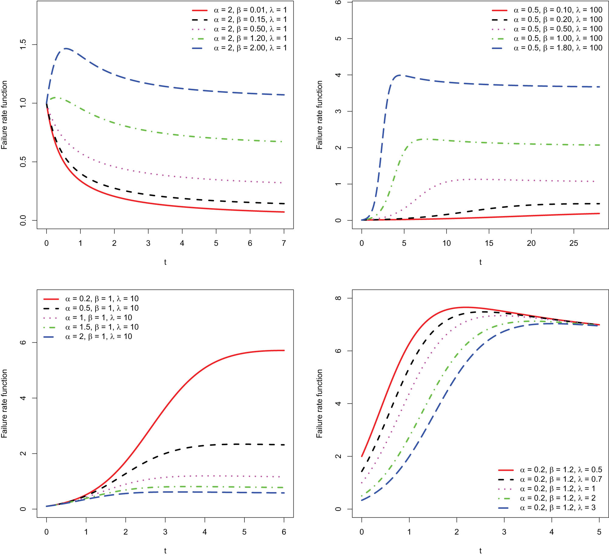
The FR function of MP for various parameter values.

On the other hand, the mean residual life (MRL) function at time t , m ( t ) , is used to evaluate the remaining mean of a random lifetime T , given the survival up to t , i.e., m ( t ) = E ( T − t | T ≥ t ) . For the MP model, the MRL can be obtained from the following relation and by the fact that as it does not have a closed form, it should be computed numerically:

m ( t ) = 1 + α λ t e β t 1 α ∫ t ∞ 1 + α λ x e β x − 1 α d x .

Another prominent reliability measure is the p -QRL function, denoted by q p ( t ) , at time t and is equal to the p th quantile of the remaining lifetime, given the survival up to t . It could be computed by

q p ( t ) = F − 1 ( 1 − ( 1 − p ) R ( t ) ) − t = Q ( t , α , β , λ ) − t ,

where Q ( t , α , β , λ ) is the solution of (6) in terms of t by replacing p with 1 − ( 1 − p ) R ( t ) . This measure should be computed numerically. The special case p = 0 . 5 is referred to as the median residual life function and is considered an alternative for the MRL in the reliability literature. Figures 3 and 4 show the MRL and median residual life for some parameter values.

Figure 3

The MRL of MP for various parameter values.

Figure 4

The median residual life function of MP for various parameter values.

In many practical problems, comparing two life distributions with respect to some of their characteristics is necessary. For example, two manufacturers may produce devices for the same purpose with different technologies, resulting in non-identical life distributions. It is then of interest to a customer to know which devices have a higher average remaining lifetime at all ages. Descriptive measures such as averages can provide a global comparative picture, although they may not be as informative as time-dependent measures in revealing inherent reliability problems. Stochastic orders give the necessary tools in such situations. For two lifetime variables T 1 and T 2 with FR functions r 1 ( t ) and r 2 ( t ) , we say that T 1 is strictly greater than T 2 in FR ordering, denoted by T 1 > T 2 , if r 1 ( t ) < r 2 ( t ) . Equivalently, T 1 > T 2 in FR ordering, if R 1 ( t ) R 2 ( t ) is strictly increasing in t ≥ 0 (see ref. [29]). If a random variable T follows from MP model with parameters α , β , and λ , then we write T ∼ MP ( α , β , λ ) for a brief notation.

Proposition 2

Assume two lifetimes T 1 ∼ MP ( α , β 1 , λ ) and T 2 ∼ MP ( α , β 2 , λ ) with β 1 < β 2 . Then, T 2 < T 1 in FR ordering.

Proof

Let R 1 and R 2 represent the reliability functions corresponding to T 1 and T 2 , respectively. Then,

R 1 ( t ) R 2 ( t ) = 1 + α λ t e β 2 t 1 + α λ t e β 1 t 1 α .

Thus, it is sufficient to show that the following function is increasing:

ζ ( t ) = 1 + α λ t e β 2 t 1 + α λ t e β 1 t .

which follows by straightforward differentiation. □

Note that Figure 2 confirms Proposition 2 graphically. As a result, under the conditions of Proposition 2, it follows that T 2 < T 1 in MRL and p -QRL orderings. For more details about ordering relationships, refer to the study of Lai and Xie [29]. Figures 2 and 3 visually confirm this result.

4 Parameter estimation

Let t 1 ≤ t 2 ≤ … ≤ t n represent an ordered, independent, and identically distributed sample of MP ( α , β , λ ) . In this section, the most well-known maximum likelihood (ML), least-squares error (LSE), and Anderson–Darling (AD) methods are discussed for estimating the parameters.

4.1 ML method

For the proposed MP model, the log-likelihood function is equal to

(7) l ( α , β , λ ; t ) = − n ln λ + ∑ i = 1 n ln ( 1 + β t i ) + β ∑ i = 1 n t i − 1 α + 1 ∑ i = 1 n ln 1 + α t i e β t i λ .

There are two common approaches to calculating the maximum likelihood estimator (MLE). In the first approach, the log-likelihood function should be maximized directly with respect to ( α , β , λ ) . In the other approach, the following likelihood equations should be solved simultaneously:

∂ ∂ α l ( α , β , λ ; t ) = 1 α 2 ∑ i = 1 n ln 1 + α λ t i e β t i − 1 α + 1 ∑ i = 1 n 1 λ t i − 1 e − β t i + α = 0 ,

∂ ∂ β l ( α , β , λ ; t ) = ∑ i = 1 n t i 1 + β t i + ∑ i = 1 n t i − 1 α + 1 ∑ i = 1 n α t i λ t i − 1 e − β t i + α = 0 ,

and

∂ ∂ λ l ( α , β , λ ; t ) = − n λ + 1 α + 1 ∑ i = 1 n α λ 2 t i − 1 e − β t i + α λ = 0 .

The observed Fisher information matrix can be computed by replacing the parameters with their corresponding estimates in the Fisher information matrix:

(8) M = − ∂ 2 ∂ α 2 − ∂ 2 ∂ α ∂ β − ∂ 2 ∂ α ∂ λ − ∂ 2 ∂ β ∂ α − ∂ 2 ∂ β 2 − ∂ 2 ∂ β ∂ λ − ∂ 2 ∂ λ ∂ α − ∂ 2 ∂ λ ∂ β − ∂ 2 ∂ λ 2 l ( α , β , λ ; t ) .

This matrix could be applied for approximating the asymptotic distribution of the MLE. Precisely, ( α ˆ − α , β ˆ − β , λ ˆ − λ ) converges in distribution to the multivariate normal N ( 0 , M − 1 ) . This point is widely used in the statistical literature for estimating the variance of the estimator and constructing confidence intervals for parameters.

4.2 LSE method

The LSE method seeks values in the parameter space, which gives the least distance from the model to the empirical distribution function. By this idea, it is natural to consider the following error function:

E 2 = ∑ i = 1 n ( F ( t i ) − F ˆ ( t i ) ) 2 .

Or, more specifically,

E 2 = ∑ i = 1 n 1 + α λ t i e β t i − 1 α − n − i n 2 .

Therefore, the LSE estimates could be obtained by

( α ˆ , β ˆ , λ ˆ ) = arg min ( α , β , λ ) ∑ i = 1 n 1 + α λ t i e β t i − 1 α − n − i n 2 .

4.3 AD method

In the AD method, every squared error term considered in the LSE approach is multiplied by a weight 1 F ( t i ) ( 1 − F ( t i ) ) . This weight boosts the effect of points in the right or left tails. Thus, the AD estimates could be computed by minimizing the sum of the weighted squared errors as follows.

( α ˆ , β ˆ , λ ˆ ) = arg min ( α , β , λ ) ∑ i = 1 n 1 F ( t i ) ( 1 − F ( t i ) ) 1 + α λ t i e β t i − 1 α − n − i n 2 .

5 Simulation study

To generate random instances from MP ( α , β , λ ) , the equation F ( X ) = U , where U is a random instance from a standard uniform distribution, is solved in terms of X ; see Eq. (6).

For every set of selected parameters, r = 1 , 000 repetitions of size n = 70 , 140 are generated. The consistency of the estimators can be checked by comparing the results for these sample sizes. Then, for every repetition, the parameters are estimated by one estimation method, and the bias (B) and the mean square error (MSE) of the estimates are computed. The simulation processes were conducted using R software and the built-in “optim” function was used for computing the optimum values of a function. The initial values that should be given as input parameters to optim function are considered to be random from a uniform distribution on intervals containing true values, for example for α in the interval ( 0 . 9 α , 1 . 1 α ) . The results of the simulations are abstracted in Tables 1 and 2. Every cell of these tables is related to one round of simulations. All estimators are clearly consistent as when the sample size increases from 70 to 140, the MSE decreases considerably. However, the MLE shows a relatively smaller MSE than other considered methods.

Table 1

Simulation results for ML, LSE, and AD methods

		n
Method	α , β , λ	70		140
		B	MSE	B	MSE
ML	2.5, 0.1, 1	0.3681	1.8034	0.1570	0.5587
		0.0498	0.0237	0.0212	0.0054
		0.0187	0.1343	0.0139	0.0624
	2, 0.05, 2	0.3935	2.0763	0.2097	0.6001
		0.0385	0.0205	0.0161	0.0027
		0.0244	0.5101	0.0064	0.2138
	1.5, 0.02, 3	0.4542	1.9537	0.1781	0.3324
		0.0308	0.0133	0.0103	0.0008
		−0.0219	0.7984	−0.0303	0.4002
LSE	2.5, 0.1, 1	0.5512	3.5541	0.2142	0.9900
		0.0982	0.0959	0.0385	0.0163
		−0.0307	0.1522	−0.0168	0.0652
	2, 0.05, 2	0.8702	4.7588	0.3794	1.3040
		0.0909	0.0709	0.0395	0.0115
		−0.1206	0.4757	−0.0504	0.2471
	1.5, 0.02, 3	0.9114	8.2305	0.3945	1.7296
		0.0952	0.1509	0.0334	0.0183
		−0.1684	0.9885	−0.1102	0.4434
AD	2.5, 0.1, 1	0.6602	4.1148	0.2437	1.0218
		0.1121	0.1097	0.0411	0.0279
		−0.0661	0.1299	−0.0175	0.0675
	2, 0.05, 2	0.8517	7.1033	0.3574	1.3689
		0.1059	0.1465	0.0369	0.0120
		−0.1124	0.5219	−0.0549	0.2321
	1.5, 0.02, 3	0.9367	7.7916	0.3328	1.0860
		0.0921	0.0994	0.0266	0.0066
		−0.2157	0.9300	−0.0998	0.4721

The first, second, and third lines of every cell are related to α , β , and λ , respectively.

Table 2

Simulation results for ML, LSE, and AD methods

		n
Method	α , β , λ	70		140
		B	MSE	B	MSE
ML	0.2, 1.5, 1	0.0884	0.3161	0.0233	0.0685
		0.3685	2.2068	0.1403	0.4688
		0.2136	0.5718	0.0856	0.0887
	0.1, 1, 2	0.0859	0.1782	0.0415	0.0452
		0.2143	0.5114	0.0970	0.1386
		0.4342	2.1459	0.1675	0.3478
	0.1, 2, 1	0.0714	0.0999	0.0387	0.0384
		0.3593	1.2824	0.2122	0.4857
		0.1728	0.2716	0.0985	0.0875
LSE	0.2, 1.5, 1	0.2345	0.9445	0.0936	0.1797
		0.6384	5.4412	0.2439	0.9048
		0.2781	1.9420	0.0800	0.1070
	0.1, 1, 2	0.2185	0.4003	0.1245	0.1322
		0.3246	0.8588	0.1804	0.2695
		0.3963	1.8814	0.2047	0.4441
	0.1, 2, 1	0.2312	0.5904	0.1190	0.1325
		0.7231	5.8993	0.3203	1.0359
		0.3289	3.0689	0.0900	0.1119
AD	0.2, 1.5, 1	0.2559	0.9260	0.1224	0.2306
		0.6587	5.3634	0.3079	1.1345
		0.2456	1.6015	0.0927	0.1301
	0.1, 1, 2	0.1722	0.2920	0.1279	0.1334
		0.2660	0.6696	0.1812	0.3002
		0.3779	1.7138	0.2093	0.5447
	0.1, 2, 1	0.2223	0.8027	0.1447	0.1900
		0.7217	7.6279	0.3961	1.5361
		0.3807	11.2221	0.1097	0.2624

The first, second, and third lines of every cell are related to α , β , and λ respectively.

6 Applications

In this section, we test the applicability and usefulness of the presented model by fitting it and some alternative models to a lifetime dataset.

6.1 Strength of single carbon fibers

In one experiment reported by Badar and Priest [30], the strength of carbon fibers is measured in GPa under tension at gauge lengths of 20 mm. This dataset, which is presented in Table 3, was analyzed in previous studies [31,32,33], among others.

Table 3

Strength (GPa) of single carbon fibers under tension at 20 mm gauges

1.312	1.314	1.479	1.552	1.700	1.803	1.861	1.865	1.944
1.997	2.006	2.021	2.027	2.055	2.063	2.098	2.140	2.179
2.253	2.270	2.272	2.274	2.301	2.301	2.359	2.382	2.426
2.382	2.478	2.554	2.514	2.511	2.490	2.535	2.566	2.570
2.800	2.773	2.770	2.809	3.585	2.818	2.642	2.726	2.697
2.633	3.128	3.090	3.096	3.233	2.821	2.880	2.848	2.818
1.966	2.240	2.435	2.629	2.648	2.821	1.958	2.224	2.434
2.954	2.809	3.585	3.084	3.012	2.880	2.848	2.684	3.067
3.433	2.586

Applying the ML method, the parameters of the MP model are estimated. It is natural to compare the MP model with the Pareto and some other Pareto generalizations. Moreover, the gamma and Weibull models are included because of their flexibility. Thus, in a comparison analysis, the alternative models. Pareto, Marshal-Olkin Pareto (MOP), Pareto exponential competing risk (PECR), gamma, Marshal-Olkin gamma (MOG), and Weibull, with the following reliability functions, are considered.

R ( t ) = 1 + α λ t − 1 α , α > 0 , λ > 0 , t ≥ 0 ,

R ( t ) = β 1 + α λ t 1 α + β − 1 − 1 , α > 0 , λ > 0 , t ≥ 0 ,

R ( t ) = 1 + α λ t − 1 α e − β t , α > 0 , β > 0 , λ > 0 , t ≥ 0 ,

R ( t ) = Γ ( α , λ t ) Γ ( α ) , α > 0 , λ > 0 , t ≥ 0 ,

R ( t ) = β Γ ( α , λ t ) Γ ( α ) − β ̅ Γ ( α , λ t ) , α > 0 , β > 0 , λ > 0 , t ≥ 0 ,

and

R ( t ) = e − λ t α , α > 0 , λ > 0 , t ≥ 0 .

Figure 5

The empirical distribution function for strength data along with estimated CDF for some alternative models.

All computations are done using the R programming language, and the “optim” function is used for optimizing the likelihood functions. Then, the Akaike information criterion (AIC), the Bayesian information criterion (BIC), the Kolmogorov–Smirnov (KS), the Cramer–von Mises (CVM), and the Anderson Darling (AD) statistics are computed for every model. Table 4 shows the results of the analysis. Based on the K-S, AD, and CVM, the MP outperforms the other models. However, the AIC of the Weibull model shows a smaller value. The Weibull and gamma, the two parameter models, give smaller BIC than other considered models. MP lies after these two models in terms of BIC but it shows better than the other three parameter models. Figure 5 draws the empirical distribution function along with the estimated CDF for MP, gamma, MOG, and Weibull distributions. Moreover, Figure 6(a) shows the histogram with an estimated PDF. Also, the FR function of the estimated MP model is presented in Figure 6(b) and shows a unimodal form.

Table 4

Results of modeling the strength data by MP and some alternative distributions

Model	α ˆ	β ˆ	λ ˆ	AIC	BIC	K-S	CVM	AD
Model	α ˆ	β ˆ	λ ˆ	AIC	BIC	p	p	p
MP	0.5787	2.6926	2464.11	108.9584	115.87	0.0531	0.0272	0.1917
MP	0.5787	2.6926	2464.11	108.9584	115.87	0.9851	0.9848	0.9925
Pareto	0.00000016	2.4776	—	286.26	290.86	0.4494	4.6711	22.13
Pareto	0.00000016	2.4776	—	286.26	290.86	0.0000	0.0000	0.0000
MOP	0.00000043	0.7633	3.2483	218.11	305.021	0.4253	4.3115	20.8400
MOP	0.00000043	0.7633	3.2483	218.11	305.021	0.0000	0.0000	0.0000
PECR	50429.5	0.4036	58,476	288.25	295.18	0.4494	4.6716	22.13
PECR	50429.5	0.4036	58,476	288.25	295.18	0.0000	0.0000	0.0000
Gamma	24.2422	9.7858	—	110.33	114.93	0.0681	0.0864	0.5643
Gamma	24.2422	9.7858	—	110.33	114.93	0.8821	0.6570	0.6818
MOG	9.7186	0.0000024	0.5383	115.17	122.08	0.0631	0.0767	0.6256
MOG	9.7186	0.0000024	0.5383	115.17	122.08	0.9301	0.7124	0.6235
Weibull	5.7404	0.0035	—	107.06	111.67	0.0675	0.0283	0.2483
Weibull	5.7404	0.0035	—	107.06	111.67	0.8890	0.9820	0.9712

Figure 6

(a) Histogram for this dataset with the estimated PDF of MP. (b) FR function of the estimated MP model.

6.2 Waiting times of bank customers

Table 5 reports 100 waiting times (in minutes) before service of bank customers. This dataset was previously analyzed in previous studies [34,35]. In a comparative analysis, the MP and the alternative models are fit to this dataset and the results are presented in Table 6. The results indicate that based on the AIC, BIC, KS, CVM, and AD statistics, the MP and gamma win the competition. Figure 7 shows the empirical CDF along with fitted CDF of MP and some alternatives, which provide a good fit. Figure 8(a) shows the histogram of the waiting times data with fitted MP PDF, which graphically shows a good fit of MP to this dataset. Moreover, in Figure 8(b), the FR function of the estimated MP distribution is plotted and shows a unimodal form.

Table 5

Waiting times (in min) of bank customers before service

0.8	0.8	1.3	1.5	1.8	1.9	1.9	2.1	2.6
2.7	2.9	3.1	3.2	3.3	3.5	3.6	4.0	4.1
4.2	4.2	4.3	4.3	4.4	4.4	4.6	4.7	4.7
4.8	4.9	4.9	5.0	5.3	5.5	5.7	5.7	6.1
6.2	6.2	6.2	6.3	6.7	6.9	7.1	7.1	7.1
7.1	7.4	7.6	7.7	8.0	8.2	8.6	8.6	8.6
8.8	8.8	8.9	8.9	9.5	9.6	9.7	9.8	10.7
10.9	11.0	11.0	11.1	11.2	11.2	11.5	11.9	12.4
12.5	12.9	13.0	13.1	13.3	13.6	13.7	13.9	14.1
15.4	15.4	17.3	17.3	18.1	18.2	18.4	18.9	19.0
19.9	20.6	21.3	21.4	21.9	23.0	27.0	31.6	33.1
38.5

Table 6

Results of modeling the waiting data by MP and some alternative distributions

Model	α ˆ	β ˆ	λ ˆ	AIC	BIC	K-S	CVM	AD
Model	α ˆ	β ˆ	λ ˆ	AIC	BIC	p	p	p
MP	4.0345	0.4753	82.5962	641.43	649.25	0.0480	0.0257	0.1653
MP	4.0345	0.4753	82.5962	641.43	649.25	0.9751	0.9883	0.9971
Pareto	0.00000011	9.8804	—	662.04	667.24	0.1729	0.7143	4.2248
Pareto	0.00000011	9.8804	—	662.04	667.24	0.0050	0.0116	0.0068
MOP	0.1095	6.7081	3.6318	645.53	653.35	0.0542	0.0497	0.4479
MOP	0.1095	6.7081	3.6318	645.53	653.35	0.9304	0.8786	0.7998
PECR	405,994	0.1011	285,836	664.04	671.86	0.1727	0.7130	4.2196
PECR	405,994	0.1011	285,836	664.04	671.86	0.0051	0.0117	0.0068
Gamma	2.0082	0.2033	—	638.60	643.81	0.0425	0.0288	0.1856
Gamma	2.0082	0.2033	—	638.60	643.81	0.9935	0.9804	0.9938
MOG	1.5715	1.9503	0.2066	642.99	650.81	0.585	0.0594	0.3736
MOG	1.5715	1.9503	0.2066	642.99	650.81	0.8827	0.8186	0.8742
Weibull	1.4584	0.0304	—	641.46	646.67	0.0577	0.0608	0.4051
Weibull	1.4584	0.0304	—	641.46	646.67	0.8929	0.8095	0.8433

Figure 7

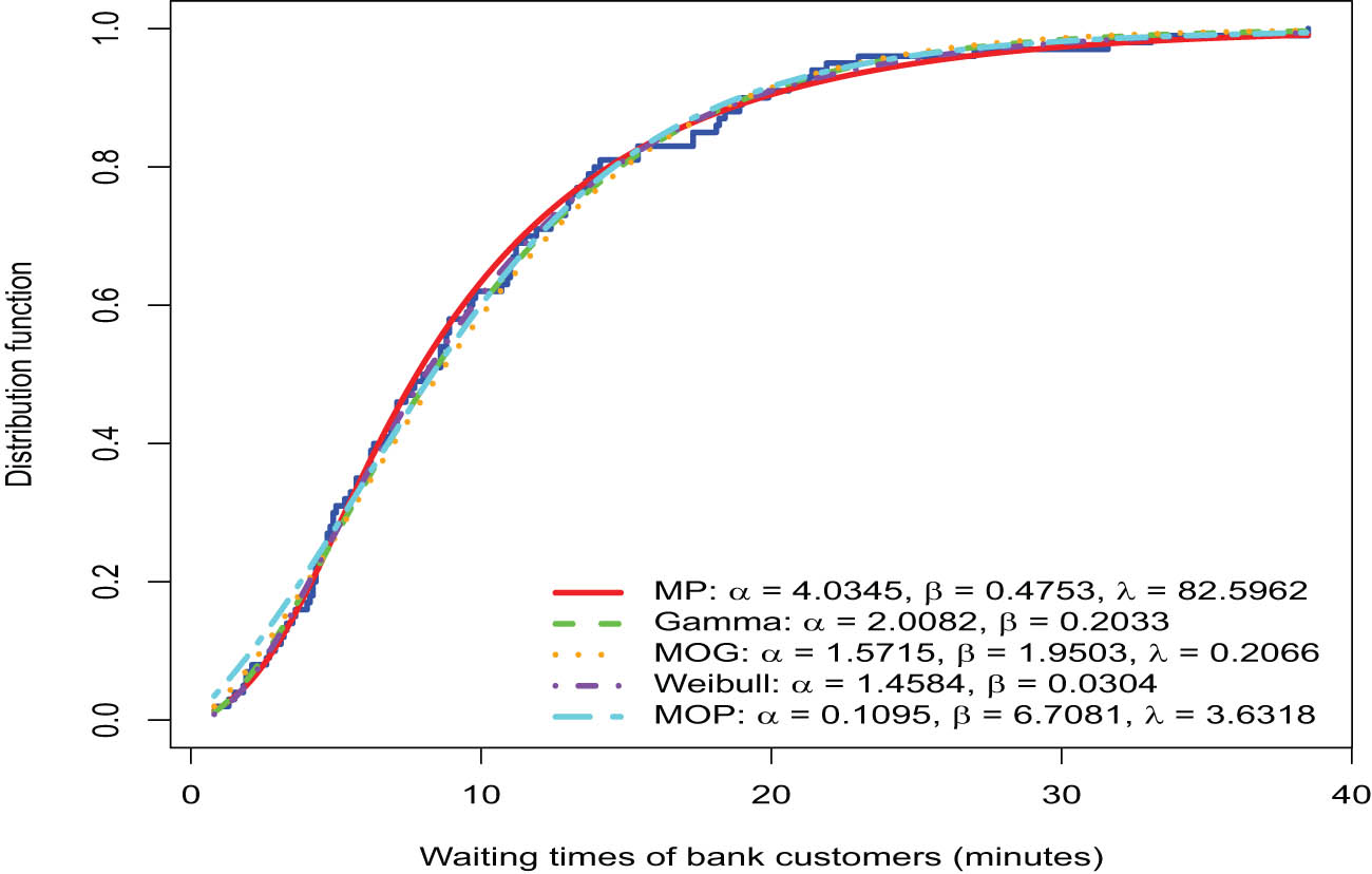
The empirical distribution function for waiting times data along with estimated CDF for some alternative models.

Figure 8

(a) Histogram for this dataset with the estimated PDF of MP. (b) FR function of the estimated MP model.

7 Conclusion

The new MP model has a relatively simple form and is flexible. It considers decreasing and upside-down FR functions. Unlike the Pareto model, the moments of this modified model are finite for all parameter values. The simulation results show that the ML, LSE, and AD estimators were consistent and efficient. However, the ML estimator provided lower MSE values. The results of fitting the MP and some alternative models to datasets of carbon fibers and bank customers’ waiting times show that the model could be useful in various applications. These results offer new concepts and applications in survival analysis, medical statistics, and risk theory. The new model will be useful to researchers in the future and will be considered a better choice than the base model. Other features and applications of the new model should be considered in future research. In particular, the following issues are interesting and open problems remain:

A bivariate family of distributions is proposed to extend the univariate case.
E-Bayesian estimation based on different censoring schemes.

Acknowledgments

The authors sincerely thank anonymous reviewers for their constructive criticism and useful suggestions, which have led to a considerable improvement in the presentation and explanations in this paper. This work was supported by Researchers Supporting Project (number: RSP2023R464), King Saud University, Riyadh, Saudi Arabia.

Funding information: This work was supported by Researchers Supporting Project (number: RSP2023R464), King Saud University, Riyadh, Saudi Arabia.
Author contributions: All authors have accepted responsibility for the entire content of this manuscript and approved its submission.
Conflict of interest: The authors state no conflict of interest.
Data availability statement: All data generated or analyzed during this study are included in this published article.

References

[1] Arnold B. Pareto distributions. 2nd edn. New York, USA: Chapman and Hall/CRC; 2015.10.1201/b18141Search in Google Scholar

[2] Newman MEJ. Power laws, Pareto distributions and Zipf’s law. Contemp Phys. 2005;46:323–51.10.1080/00107510500052444Search in Google Scholar

[3] Barranco-Chamorro I, Jiménez-Gamero MD. Asymptotic results in partially non-regular log-exponential distributions. J Stat Comput Simul. 2012;82(3):445–61.10.1080/00949655.2010.540578Search in Google Scholar

[4] Burroughs SM, Tebbens SF. Upper-truncated power law distributions. Fractals. 2001;9:209–22.10.1142/S0218348X01000658Search in Google Scholar

[5] Schroeder B, Damouras S, Gill P. Understanding latent sector error and how to protect against them. ACM Trans. 2010;6:1–14.10.1145/1837915.1837917Search in Google Scholar

[6] Bak P, Sneppen K. Punctuated equilibrium and criticality in a simple model of evolution. Phys Rev Lett. 1993;24:4083–6.10.1103/PhysRevLett.71.4083Search in Google Scholar PubMed

[7] Sornette D. Multiplicative processes and power laws. Phys Rev E. 1998;57:4811–13.10.1103/PhysRevE.57.4811Search in Google Scholar

[8] Carlson JM, Doyle J. Highly optimized tolerance: A mechanism for power laws in designed systems. Phys Rev E. 1999;60:1412–27.10.1103/PhysRevE.60.1412Search in Google Scholar PubMed

[9] Akinsete A, Famoye F, Lee C. The beta-Pareto distribution. Stats. 2008;42:547–63.10.1080/02331880801983876Search in Google Scholar

[10] Mahmoudi E. The beta generalized Pareto distribution with application to lifetime data. Math Comput Simul. 2011;81:2414–30.10.1016/j.matcom.2011.03.006Search in Google Scholar

[11] Nassar MM, Nada NK. The beta generalized Pareto distribution. J Stat Adv Theory Appl. 2011;3:1–17.Search in Google Scholar

[12] Alzaatreh A, Famoye F, Lee C. Gamma-Pareto distribution and its applications. J Mod Appl Stat Methods. 2012;11:78–94.10.22237/jmasm/1335845160Search in Google Scholar

[13] Zea LM, Silva RB, Bourguignon M, Santos AM, Cordeiro GM. The beta exponentiated Pareto distribution with application to bladder cancer susceptibility. Int J Stat Prob. 2012;1:8–19.10.5539/ijsp.v1n2p8Search in Google Scholar

[14] Bourguignon M, Silva RB, Zea LM, Cordeiro GM. The Kumaraswamy Pareto distribution. JSTA. 2013;12:129–44.10.2991/jsta.2013.12.2.1Search in Google Scholar

[15] ElbataL I. The Kumaraswamy exponentiated Pareto distribution. Econ Qual Control. 2013;28:1–9.10.1515/eqc-2013-0006Search in Google Scholar

[16] Papastathopoulos I, Tawn JA. Extended generalized Pareto models for tail estimation. J Stat Plan. 2013;143:131–43.10.1016/j.jspi.2012.07.001Search in Google Scholar

[17] Mead M. An extended Pareto distribution. Pak J Stat Oper Res. 2014;10:313–29.10.18187/pjsor.v10i3.766Search in Google Scholar

[18] Korkmaz MC, Altun E, Yousof HM, Afify AZ, Nadarajah S. The Burr X Pareto distribution: Properties, applications and var estimation. J Risk Financ Manag. 2018;10:1–16.10.3390/jrfm11010001Search in Google Scholar

[19] Elbatal I, Aryal G. A new generalization of the exponential Pareto distribution. J Inf Optim Sci. 2017;5:675–97.10.1080/02522667.2016.1220079Search in Google Scholar

[20] Tahir A, Akhter AS, Haq MA. Transmuted new Weibull-Pareto distribution and its applications. Appl Appl Math. 2018;13:30–46.Search in Google Scholar

[21] Ghitany ME, Gómez-Déniz E, Nadarajah S. A new generalization of the Pareto distribution and its Application to insurance data. J Risk Financ Manag. 2018;2:1–15.10.3390/jrfm11010010Search in Google Scholar

[22] Ihtisham S, Khalil A, Manzoor S, Khan SA, Ali A. Alpha-Power Pareto distribution: Its properties and applications. PLoS One. 2019;5:1–21.10.1371/journal.pone.0218027Search in Google Scholar PubMed PubMed Central

[23] Haj Ahmad H, Almetwally E. Marshall-Olkin generalized Pareto distribution: Bayesian and Non-Bayesian estimation. Pak J Stat Oper Res. 2020;16:21–33.10.18187/pjsor.v16i1.2935Search in Google Scholar

[24] Jayakumar K, Krishnan B, Hamedani GG. On a new generalization of Pareto distribution and its applications. Commun Stat Simul. 2020;49:1264–84.10.1080/03610918.2018.1494281Search in Google Scholar

[25] Jayakumar K, Kuttykrishnan AP, Krishnan B. Heavy tailed Pareto distribution: properties and applications. J Data Sci. 2021;18:828–45.10.6339/JDS.202010_18(4).0015Search in Google Scholar

[26] Lai CD, Xie M, Murthy DNP. A modified Weibull distribution. IEEE Trans Reliab. 2003;52:33–7.10.1109/TR.2002.805788Search in Google Scholar

[27] MacGillivray HL. Skewness and asymmetry: Measures and orderings. Ann Stat. 1986;14:994–1011.10.1214/aos/1176350046Search in Google Scholar

[28] Moors J. A quantile alternative for kurtosis. J R Stat Soc Ser D-(Stat). 1988;562:25–32.10.2307/2348376Search in Google Scholar

[29] Lai CD, Xie M. Stochastic ageing and dependence for reliability. New York, USA: Springer; 2006.Search in Google Scholar

[30] Badar MG, Priest AM. Statistical aspects of fiber and bundle strength in hybrid composites. In: Hayashi T, Kawata K, Umekawa S, editors. Progress in Science and Engineering Composites. ICCM-IV, Tokyo; 1982. p. 1129–36.Search in Google Scholar

[31] Kundu D, Raqab MZ. Estimation of R=P(Y<X)for three-parameter Weibull distribution. Stat Probab Lett. 2009;79:1839–46.10.1016/j.spl.2009.05.026Search in Google Scholar

[32] Afify AZ, Cordeiro GM, Butt NS, Ortega EMM, Suzuki AK. A new lifetime model with variable shapes for the hazard rate. Braz J Probab. 2017;31:516–41.10.1214/16-BJPS322Search in Google Scholar

[33] Nada A, Ahmed M, Gemeay M, Aljohani HM, Afify AZ. The extended log-logistic distribution: Inference and actuarial applications. Mathematics. 2021;9(12):1–22.10.3390/math9121386Search in Google Scholar

[34] Ghitany ME, Atieh B, Nadarajah S. Lindley distribution and its application. MACSI. 2008;78:493–506.10.1016/j.matcom.2007.06.007Search in Google Scholar

[35] Shanker R. On generalized Lindley distribution and its applications to model lifetime data from biomedical science and engineering. Insights Biomed. 2016;1(2):12. 10.21767/2572-5610.100012.Search in Google Scholar

Received: 2023-04-08

Accepted: 2023-06-07

Published Online: 2023-07-14

This work is licensed under the Creative Commons Attribution 4.0 International License.

Articles in the same Issue

https://doi.org/10.1515/phys-2022-0266

Keywords for this article

power-law models; maximum likelihood estimation; mean square error estimation

Creative Commons

BY 4.0