Controlling the physical field using the shape function technique

ThanhTrung Trang; ThanhLong Pham; Yueming Hu; Weiguang Li; Shoujin Lin

doi:10.1515/phys-2022-0249

Artikel Open Access

Controlling the physical field using the shape function technique

ThanhTrung Trang , ThanhLong Pham , Yueming Hu , Weiguang Li und Shoujin Lin

Veröffentlicht/Copyright: 21. Juni 2023

Veröffentlicht von

Veröffentlichen auch Sie bei De Gruyter Brill

Manuskript einreichen Informationen für Autor*innen Erkunden Sie dieses Fachgebiet

Aus der Zeitschrift Open Physics Band 21 Heft 1

Abstract

A field is described as a region under the influence of some physical force, such as electricity, magnetism, or heat. It is a continuous distribution in the space of continuous quantities. The characteristics of the field are that the values vary continuously between neighboring points. However, because of the continuous nature of the field, it is possible to approximate a physical field of interpolation operations to reduce the cost of sampling and simplify the calculation. This article introduces the modeling of the parametric intensity of physical fields in a general form based on the interpolation shape function technique. Besides the node points with sample data, there are interpolation points, whose accuracy depends significantly on the type of interpolation function and the number of node points sampled. Therefore, a comparative analysis of theoretical shape functions (TSFs) and experimental shape functions (ESFs) is carried out to choose a more suitable type of shape function when interpolating. Specifically, the temperature field is the quantity selected to apply, analyze, and conduct experiments. Theoretical computations, experiments, and comparisons of results have been obtained for each type of shape function in the same physical model under the same experimental conditions. The results show that ESF has an accuracy (error of 0.66%) much better than TSF (error of 10.34%). Moreover, the field model surveyed by a generalized reduced gradient algorithm allows for identifying points with the required parameter values presented in detail. The illustrated calculations on temperature field control in the article show that the solution for both forward and reverse problems can be determined very quickly with high accuracy and stability. Therefore, this technique is expected to be entirely feasible when applied to thermal control processes such as drying in paint technology, kilns, and heat dissipation in practice.

Keywords: physical field; control; thermal; shape function; reversibility problem

1 Introduction

In engineering, the presence of physical fields such as temperature, electromagnetism, sound, and light is prevalent. They are continuous quantities whose values vary in space. Except in realistic situations, these physical fields are intentionally created by technology. They are usually maintained by controlled emitters to control the field’s energy for the design engineer’s specific purpose. The values of these quantities gradually decrease from the emitter’s source to the field’s boundary. There are also complex superposition effects for fields with multiple sources, in which specific rules determine the parameter intensity at points in the field.

Due to the invisible nature of these fields, when one wants to determine a physical field area with specific characteristics, it is necessary to have specialized equipment, which is often expensive to measure, or many sensors to arrange to obtain accurate results. Oktavia has used this approach in his research. They used five sensors combined with a spatial interpolation concept to control the temperature and humidity of the data center environment [1]. Riederer et al. presented the mathematical model choices suitable for studying the influence of sensor position in the construction of temperature field control [2]. C-Bam-bang-Dwi et al. researched an automatic intelligent wireless climate sensor button to control indoor temperature and humidity to improve the quality of life [3]. By using the same idea, Silveira et al. used a wireless sensor network to control room temperature [4]. Kumar et al. also developed a sensor button system, but unlike Silveira, they used the IEEE 1,451 standards to monitor room temperature [5]. Kim et al. developed an outdoor air temperature fault sensor for machine learning based air handler fault detection and diagnosis [6]. The model is applied to control the temperature of the outdoor air.

The second most common way is to investigate these fields through hypothetical mathematical models. Some prominent recent studies based on this idea include that of Ertuk et al., who used the theory of fractional analysis to study the motion of a beam on a bent nanowire [7]. Jajarmi et al. used the classical Lagrange method to study the complex displacement and charge of a microdynamics condenser system [8]. Most recently, Baleanu et al. used the structure of fractional and integral derivatives to investigate the general fractional model of COVID-19, studying the effects of isolation and quarantine [9]. Similarly, Jajarmi et al. investigated the asymptotic behavior of immune tumor dynamics using the general fractional model [10].

As mentioned above, temperature is one of many physical quantities associated with life around us. Therefore, the study of temperature field control has received the attention of many researchers. Piotr and Je Drysiak investigated the problem of heat conduction in a two-phase laminate made of microplates periodically distributed along one direction [11]. Francesco and Pierre-Louis investigated strategies to control nanoclusters’ shape change by varying the external environment’s optimal temperature [12]. Jiang et al. used the radial integration boundary element method in conjunction with a modified Levenberg-Marquardt algorithm to reconstruct the shape in transient thermal conduction problems [13]. Yang et al. studied the finite element electrothermal coupling method based on the radial point interpolation method (RPIM) to monitor the efficiency of thermoelectric coupling [14]. In this problem, Joule heat is often used as the sole heat source in the heat field, and the calculation of Joule heat depends on the intensity of the first-order variation of the electric field. Therefore, the idea of the study is to use the first-order continuous RPIM to interpolate variables in the survey domain. Feppon et al. used Hadamard’s method of shape differentiation to optimize the shape and topology for weakly coupled three physics problems, including heat propagation, fluid flow, and structural deformation [15]. Hobiny and Abbas used the finite element technique to study the thermal diffusion interaction in an unbound material with the cavity sphere in the context of a double-phase hysteresis model [16].

The general idea of thermal field research and control methods is to model the properties of the thermal field and use different algorithms that combine measurements at several key points to control the thermal field. Every model is an idealization of the real world; as George Box said, “All models are wrong, some are useful” [17]. One of the ideal solutions for modeling and controlling thermal field data is the use of the spatial shape function interpolation method. It is a method of estimating the value of unknown data points within the range of a discrete set containing several known data points with an estimated accuracy. The use of this method to control the temperature field has attracted the attention of many researchers. Wang et al. used the surface spline interpolation method with non-uniform thermal sensor placement to study and control the temperature in integrated circuits. The researchers experimented with reconstructing the full thermal status of a 16-core processor. [18]; Bullo et al. used quadratic interpolation to accurately calculate the thermal field distribution computation, especially in complex biological structures, which are easily encountered in predictions of heat distributions obtained in hyperthermic treatments [19]; and Thanh et al. used the shape function to compute the distribution for the temperature field. However, the reversibility problem has not been mentioned or solved yet [20]. Tang et al. uses continuous gradient smoothed GFEM (SGFEM) combined with a higher-order finite element shape function to solve the problems of heat transfer and thermoelectricity [21]. The higher-order finite element shape function ensures the continuity of the gradient between the elements. Through four typical numerical examples, including stable, transient, and thermoplastic heat transfer, the advantages of the method have been demonstrated in terms of accuracy, convergence rate, stability, and efficiency. Klimczak and Cecot used a multiscale finite element method (FEM) based on the particular shape function assessment model of steady-state heat transfer in heterogeneous materials. However, the result is still imperfect, and the method error is approximately 2% [22]. Most recently, Pucciarelli and Ambrosini used the shape function approach to predict degraded heat transfer to supercritical pressure fluids in nuclear reactors [23].

As summarized and analyzed above, it can be seen that all the research to control thermal field control has only addressed the one-dimensional problem (also known as the forward problem) without any research simultaneously solving the thermal field control for both forward and reverse problems. Specifically, the content of this reversibility problem will be detailed in Section 4. Therefore, supplementation of this deficiency reverse problem is the first motivation for the authors to carry out this study.

Furthermore, the precision of interpolation strongly depends on the continuity of the interpolated quantity, the density of the sample points, and especially the type of function used in the calculation process [1,18,19]. The error caused by the function form when interpolating is a method error. Determining the correct approximation function form is essential when the density of the sample points is not large enough. This is especially important when the cost of sampling is high. To the authors’ knowledge, other studies have yet to delve into comparative analysis to choose which approximation function form is the most suitable for thermal field interpolation. According to Thanh et al. [20], the theoretical shape function (TSF) is applied effectively to machine tool error interpolation, but there is no verification in the field of thermal interpolation. According to Hoe [24], the experimental shape function (ESF) has a rather complicated process, but what is the result compared to the TSF in solving the thermal field parameter control problem? Answering this question is the second motivation for the authors to carry out this research.

The content of this article focuses on the following aspects: First, to model a multisource field using a shape function method, namely the temperature field, design and implement experiments, and compare and verify the accuracy of TSF and ESF. Second, solve the problem of reversibility for the temperature field to find the coordinates of the points with a given intensity. Third, use the generalized reduced gradient algorithm (GRG) to find the temperature field’s maximum and minimum intensity points with high accuracy and stability.

The novelty of this article is the analysis of results from practical experiments to select the kind of shape function with high accuracy that is more suitable for the thermal control problem. In our previous articles, when applying the shape function method to model and graph the Wi-Fi wave field [25], based on experimental results, we also commented on the difference in results when using two kinds of shape function forms. However, the authors have yet to go into deep research and analysis to find the reasons for this deviation. Therefore, the authors continue to investigate and apply it to the heat transfer phenomenon to find the answer.

The second novelty is that it confirms which types of shape functions, with high accuracy and practical application, solve heat transfer issues in both forward and reverse directions. The research team also applies the GRG method to calculate the points with the maximum and minimum temperature intensity in quick time for high accuracy and stability, which is entirely feasible when applied in practice to control the thermal field.

The article is organized as follows: Section 2 introduces the concepts of the shape function, the TSF, and the ESF. Section 3 presents a case study on the temperature field’s design and experimentation for selecting the appropriate shape function form and discusses why there is a difference in accuracy between TSF and ESF. Next, forward and reverse problems of the physical field’s control and solutions are detailed in Section 4. Then, the temperature field experiment is again used to calculate the illustration of the control reversibility issue and compare and verify the design. Finally, Section 6 is the conclusion of this study and the proposal for further research.

2 TSF and ESF

2.1 Concept of a shape function

The shape function is the function that interpolates the solution between the discrete values obtained at the mesh nodes. This form of function is very commonly used in interpolation [26], and especially for FEM, the role of the shape function (also known as the trial function or the basis function) is essential. Depending on different problems, the shape function will have many different forms. Low-order polynomials are typically chosen as shape functions. The higher the order of the shape function, the more complex the shape of the element, the stronger the adaptability of the element, the fewer the number of elements needed to solve the interpolation problem, and the fewer balanced equations. Hence, the order of the balanced equations is lower, and it takes less time to solve the system of equations. However, when the order of the shape function is increased, the calculation of the discrete matrix becomes more complicated. Therefore, there is a most suitable order for each problem, which can make the total calculation time more economical. This generally needs to be determined based on the engineer’s computational experience.

Consider a field consisting of n influential scalar sources in the survey space, where F i is the influence coefficient of the i th source on the survey point P i in that space (Figure 1).

Figure 1

Describe the influence of key points on the survey point through the shape function.

Let δ i be the intensity of the survey parameter at the i th source, which is the value measured by simple measurements. Then, ( F i δ i ) represents the quantitative value of the influence of source n i on point P i under consideration in an independent way, separate from other sources of influence. If considering the simultaneous influence of all n influence sources acting on point P i , the superposition parameter at point P i is:

(1) δ p i = F 1 ( i ) δ 1 + F 2 ( i ) δ 2 + ⋯ + F n ( i ) δ n ,

where F i is the stationary value of the shape function at the i th source, with i = 1 , … , n .

F i needs to satisfy the following conditions:

At node i , F i = 1 ; at other nodes, F i = 0 ;
It can guarantee the continuity between adjacent units of the unknown quantity ( u , v or x , y ) defined by it;
It should contain any linear term, and the element defined by it can only satisfy the constant strain condition.

There are two ways to determine the functions of the form F i in Eq. (1): TSF and ESF.

2.2 TSFs

For three-dimensional finite element simulations, it is convenient to discretize the simulation domain using tetrahedrons or boxes, as depicted in Figure 2.

Figure 2

The key points and reference systems in the survey area. (a) Tetrahedral original coordinate system, (b) tetrahedral transformed coordinate system, and (c) box finite elements.

In this article, the author presents the simulation domain of the survey area as a box. The tetrahedron is implemented similarly.

According to Hoe [24], the TSF for the eight key points of the box-shaped survey area is as follows:

(2) F 1 = 1 8 ( 1 + r ) ( 1 − s ) ( 1 + t ) , F 2 = 1 8 ( 1 + r ) ( 1 + s ) ( 1 + t ) , F 3 = 1 8 ( 1 − r ) ( 1 + s ) ( 1 + t ) , F 4 = 1 8 ( 1 − r ) ( 1 − s ) ( 1 + t ) , F 5 = 1 8 ( 1 + r ) ( 1 − s ) ( 1 − t ) , F 6 = 1 8 ( 1 + r ) ( 1 + s ) ( 1 − t ) , F 7 = 1 8 ( 1 − r ) ( 1 + s ) ( 1 − t ) , F 8 = 1 8 ( 1 − r ) ( 1 − s ) ( 1 − t ) .

The formula for transforming the axis to the reference system ( r , s , t ) , whose origin is at the center of the box, is:

(3) r = x − x ∗ a , s = y − y ∗ b , t = z − z ∗ c ,

where a , b , and c are the units of length that describe the width, length, and height of the box and is determined according to Figure 2(c). The coordinates of the center of gravity of the element under consideration are as follows:

(4) x ∗ = x 1 + x 4 2 , y ∗ = y 1 + y 2 2 , z ∗ = z 1 + z 3 2 .

It can be seen that the values ( r , s , t ) vary in the range [ − 1 , 1 ], so after transforming, the F i values also change in the range [ − 1 , 1 ]. Performing such a coordinate transformation significantly simplifies the practical implementation of the FEM.

2.3 ESFs

The F i values in Eq. (1) are the stationary values or influence coefficients of the coordinate function f i ( x , y , z ) , which is a function of the distances of the respective coordinates.

(5) f 1 ( x , y , z ) P i = F 1 ⋮ f n ( x , y , z ) P i = F n i = 1 , … , n .

Function f i ( x , y , z ) is called the ESF, and F i is the influence coefficient of these functions acting on the survey point P i .

Suppose to investigate a point P i of known intensity δ P i , with components of the measurement data including δ P i = ( d x , d y , d z , φ x , φ y , φ z ) ( P i ) influenced by a field of n key points with intensity ( δ 1 , δ 2 , … , δ n ) . In which, in the general case, a point in space needs to be surveyed with six components: three coordinates ( d x , d y , d z ) and three rotation angles ( φ x , φ y , φ z ) .

The relationship of the intensity of known key points with the data components of the survey point P i is as follows:

(6) δ 1 P i = F 1 d x ( 1 ) + F 2 d x ( 2 ) + … + F n d x ( n ) ⋮ δ n P i = F 1 φ z ( 1 ) + F 2 φ z ( 2 ) + … + F n φ z ( n ) .

The influence coefficients of the ESF of n key points on point P i are determined as follows:

(7) F 1 ⋮ F n P i = d x ( 1 ) ⋯ d x ( n ) ⋱ φ z ( 1 ) ⋯ φ z ( n ) − 1 d x P i ⋯ φ z P i .

The general ESF cannot be determined by a single set of influence coefficients as Eq. (7). Therefore, it is necessary to investigate more than m survey points to obtain m sets of influence coefficients of ESF as in Eq. (8). The number of survey points m more or less often depends on the problem type and calculation experience, as described above. Of course, the larger the number of survey points m , the greater the accuracy of the ESF, but the higher the cost.

(8) F 1 ⋮ F n P 1 , F 1 ⋮ F n P 2 , … , F 1 ⋮ F n P m .

After determining m sets of influence coefficients of the shape functions, through regression to calculate the ESF at the i th source as follows:

(9) ( F P 1 ( i ) , F P 2 ( i ) , … , F P m ( i ) ) ⇒ f i ( x , y , z ) .

3 Case study and select the appropriate shape function form

As analyzed above, there are two ways to determine the shape function for a physical field, but which type of function has higher accuracy and which type of function is more convenient to use? The content of this section will help us obtain the most suitable answer. It is easy to see that the interpolated value (Eq. (1)) calculated according to TSF (Eq. (2)) and ESF (Eq. (9)) with the same intensity survey key points will be difficult to equal. If we design an experiment to compare these two types of functions and independently verify the interpolation results, we will know the accuracy of each kind of function.

3.1 Experiment design

Design a box-shaped survey space as shown in Figure 2(c) with the following dimensions: 2 a = 500 (mm), 2 b = 400 (mm), 2 c = 380 (mm).

Two cooling fans are arranged at both ends of the greenhouse with a capacity of 2.5 W/unit.

Eight thermal sources were set up at eight peaks of the greenhouse model, using 10 W/bulb halogen bulbs to generate heat. The light bulb is constantly on and running at total capacity. Furthermore, eight temperature sensors are placed close to the eight peaks of the greenhouse model, which coincides with the location of eight thermal sources. This allows for continuous monitoring of the installed temperature.

Use an internal portable thermal sensor to measure the temperature at any point in the survey space to calculate and compare the interpolated results (Figure 3(a)).

Figure 3

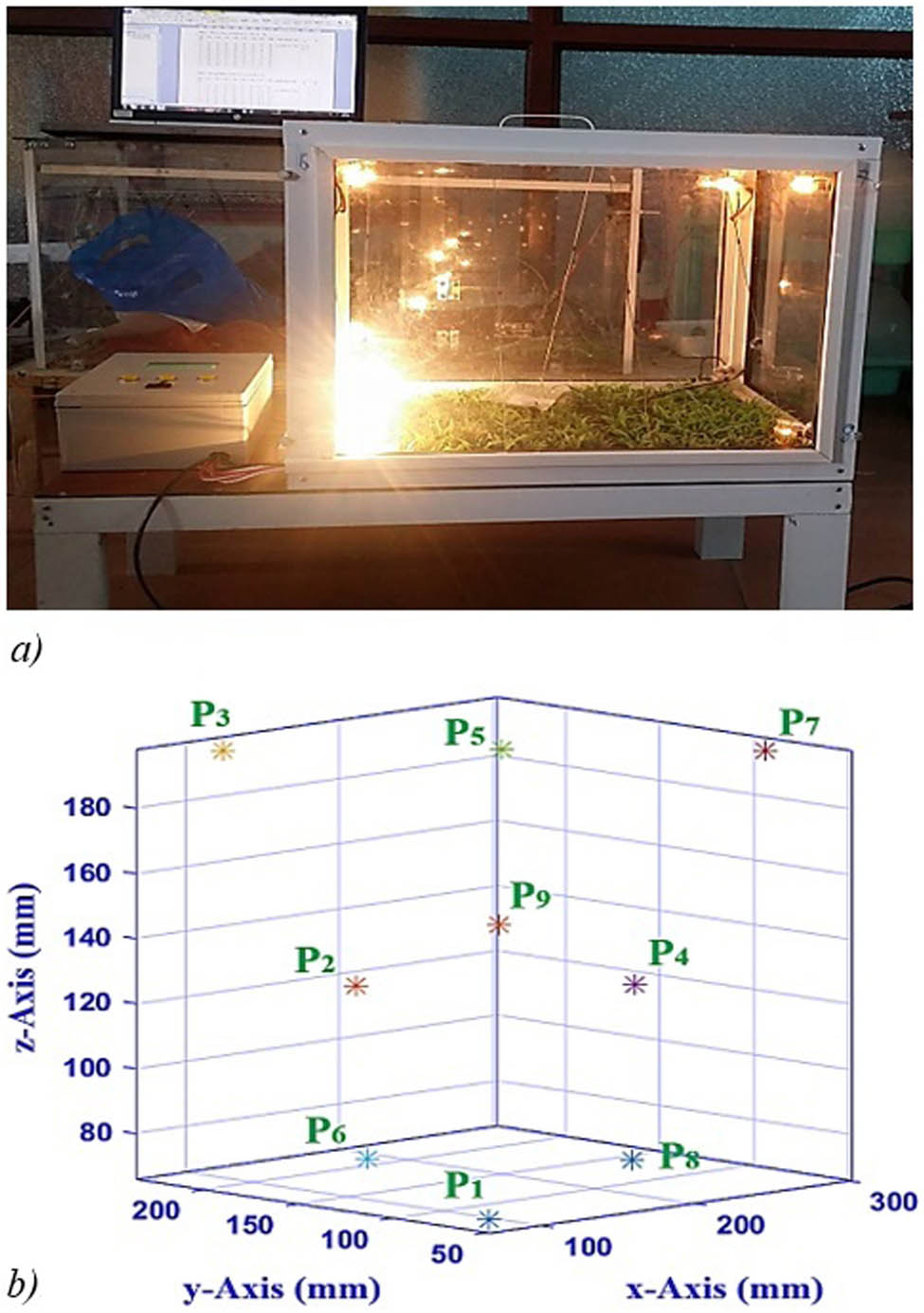
(a) Experimental model and (b) nine internal temperature survey points.

3.2 Measurement sensor

The LM35 sensor is a precision integrated circuit temperature device, and its robust construction makes it suitable for various environmental conditions. The output voltage is linearly proportional to the temperature in degrees Celsius. It does not require any external component to calibrate the circuit and has a typical accuracy of ±1/4°C at room temperature and ±3/4°C over a whole −55 to 155°C temperature range. It has an operating voltage of 4–30 V, and since the LM35 device draws only 60 μ A from the supply, it has a very low self-heating of less than 0.1°C in still air. All of this makes it perfect for applications such as power supplies, battery management, heating, ventilation, air conditioning, and appliances.

The LM35 temperature sensor uses the basic principle of a diode to measure known temperature values. As we all know from semiconductor physics, the voltage across a diode increases at a known rate as the temperature increases. By accurately amplifying the voltage change, we can quickly generate a voltage signal directly proportional to the surrounding temperature. The internal schematic of the LM35 temperature sensor IC is according to the datasheet, as shown in Figure 4.

Figure 4

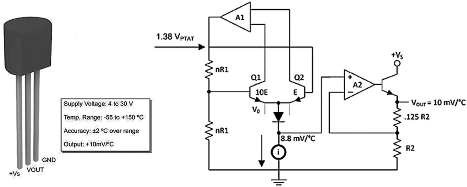
Temperature sensor used in the experiment.

Figure 5 is a circuit that displays temperature parameters using LM35 and Arduino UNO.

Figure 5

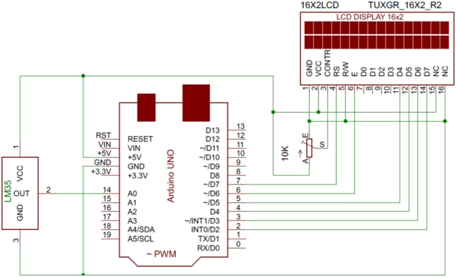
Circuit to display temperature parameters using LM35 and Arduino UNO.

With the above advantages and thermal errors, compared to the measurement using expensive thermal imaging cameras, the experiment using the LM35 temperature sensor with Arduino UNO completely meets the desired accuracy.

3.3 Experiment and results

Conduct a survey to measure the temperature at nine points ( P 1 , P 2 , … , P 9 ) as designed in the survey space (Figure 3(b)). The average results after ten times of experiments and measurement and interpolation results calculated according to two methods of TSF and ESF, are shown in Table 1 and Figure 6.

Table 1

The interpolation results calculated according to TSF and ESF; the average experiment results and error of each function form

Points	x (mm)	y (mm)	z (mm)	TSF (°C)	ESF (°C)	The average experiment results (°C)	Error of TSF (%)	Error of ESF (%)
P1	95	71	66	33.72	31.09	31.12	7.71	0.1
P2	95	142	132	35.5	31.3	31.64	10.87	1.09
P3	95	213	198	35.81	30.38	30.14	15.83	0.79
P4	190	71	132	35.26	31.35	31.66	10.21	0.99
P5	190	142	198	36.06	32.54	32.76	9.15	0.68
P6	190	213	66	34.73	31.48	31.4	9.59	0.25
P7	275	71	198	35.76	31.9	31.72	11.3	0.56
P8	275	142	66	36.2	31.26	31.55	12.85	0.93
P9	275	213	132	33.05	31.4	31.23	5.51	0.54
Average error			10.34	0.66

Figure 6

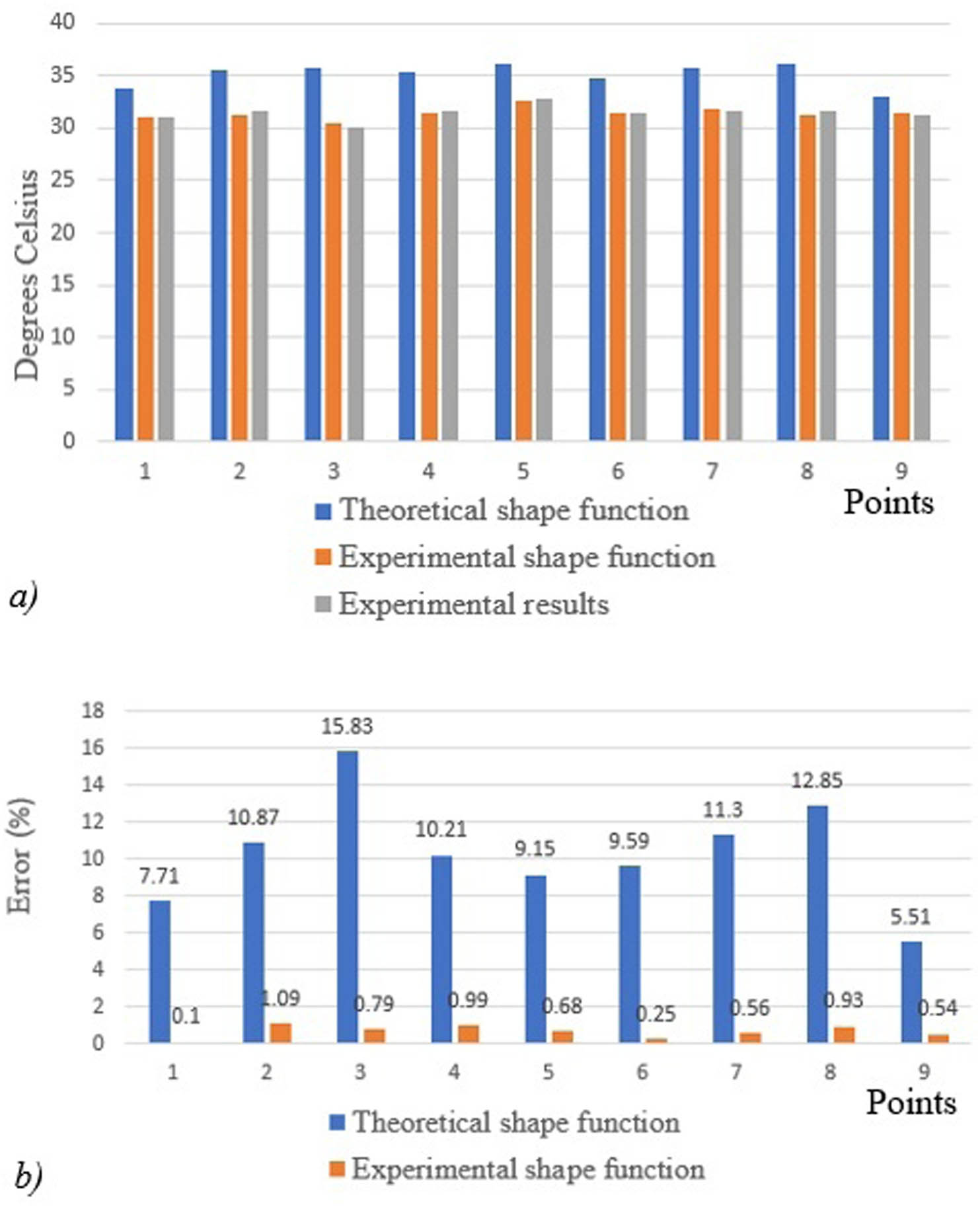
The interpolation results calculated according to TSF and ESF, compared with (a) experimental results and (b) accuracy of each function form.

3.4 Discussion

At the interpolation points in Figure 6, because no key points are shown, it can be seen that there is no overlap in values between TSF and ESF, which can be realized from the mathematical model as analyzed in Section 2.

The TSF exhibits symmetry in the interpolation spatial texture, which is very convenient to use due to its availability. However, in practice, the key points are not always symmetrically arranged in the survey space, and not all fields are symmetrical in the influence region. Moreover, the experimental results show that, in the same field of influence under the same conditions, the accuracy of the ESF (an error of 0.66%) is always superior to that of the TSF (an error of 10.34%). The results will always be the same at the measurement sampling points. Therefore, it can be seen that the error is due to using an incorrect calculation functional form.

4 Forward and reverse problems of the physical field’s control

In Section 3, it was proved that the field model using ESF would give results with higher accuracy than TSF. After determining the general expression of the shape functions from Eq. (9), this mathematical model will have two reversible problems.

4.1 Forward problem

Given each key point’s coordinates and parametric intensity, determine the parameter intensity at any given point.

The manner to solve the forward problem is as follows: to know the coordinates of a point P i ( x i , y i , z i ) in the survey space, the coordinates and the intensity at the sources δ i , i = 1 , … , n . First, it is necessary to determine the influence coefficients of each source according to Eq. (5), then use Eq. (1) to determine the parameter intensity at the requirement point P i ( x i , y i , z i ) , as illustrated in Section 3.

4.2 Reverse problem

Given each key point’s coordinates and parametric intensity, find the coordinates of the points with a given intensity and the field’s maximum and minimum parameter strengths.

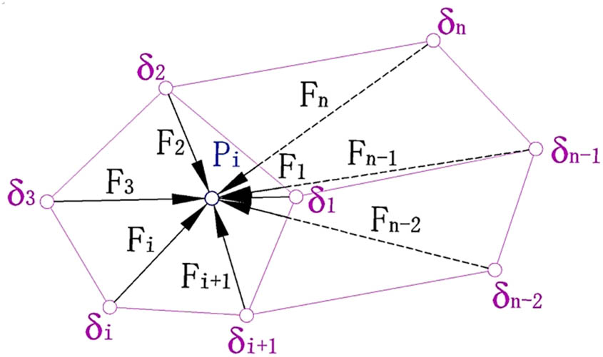
The way to solve the reverse problem is as follows: as shown in Figure 1, when P i ( x i , y i , z i ) changes position, the shape functions ( F 1 , F 2 , … , F n ) i also change and Eq. (1) describes only the effect of n sources on a point P i ( x i , y i , z i ) . Suppose we investigate a set of points located inside the field n source ( δ 1 , δ 2 , … , δ n ) , with all ( n + 1 ) values of parameter ( δ 1 , δ 2 , … , δ n , δ p i ) ’s intensity known through measurement. At a survey point P i ( x i , y i , z i ) , keeping the shape functions unchanged ( F 1 , F 2 , … , F n ) i , only changing the intensity of the source will have the following relationship:

(10) δ P i ( 1 ) = F 1 δ 1 ( 1 ) + F 2 δ 2 ( 1 ) + … + F n δ n ( 1 ) ⋮ δ P i ( n ) = F 1 δ 1 ( n ) + F 2 δ 2 ( n ) + … + F n δ n ( n ) .

The problem requires determining a point or a set of points with an intensity δ k lying inside the field. This is a widespread engineering issue, especially in heat transfer, drying, furnaces, heat dissipation, etc.

Let the point P k ( x k , y k , z k ) of intensity δ k be the point to be found. Then, according to Eq. (9), these coordinate variables ( x k , y k , z k ) are in the shape function and have the relation Eq. (1) written for the point P k as follows:

(11) δ k = F 1 ( k ) δ 1 + F 2 ( k ) δ 2 + … + F n ( k ) δ n .

The expanded form of this expression is as follows:

(12) δ k = f 1 ( k ) δ 1 + f 2 ( k ) δ 2 + … + f n ( k ) δ n .

The problem is converted to the equivalent form using the GRG [27] method as Eq. (13):

(13) A = ∑ i = 1 n [ f 1 ( k ) δ 1 + f 2 ( k ) δ 2 + … + f n ( k ) δ n − δ k ] 2 ⇒ min , x min ≤ x ≤ x max , y min ≤ y ≤ y max , z min ≤ z ≤ z max .

The solution of problem Eq. (13) is the set of points P k ( x k , y k , z k ) with the same intensity value δ k to be found.

5 Case study with temperature problem

Return to the temperature-space survey as illustrated in Section 3. Assume that these heat sources are always constant and equal to the preset value (no loss in heat exchange with the environment) and that the sampling time is long enough for good heat transfer. Conduct experiments at any eight points in the survey space to build a system of equations to determine the influence coefficients of the ESF such as Eq. (7). The results are presented in Table 2.

Table 2

Relationship between the survey point and the influence coefficient in the stationary state

x (mm)	y (mm)	z (mm)	F1	F2	F3	F4	F5	F6	F7	F8
125	100	0	0.189	0.0792	0.1933	0.5619	0.0024	−0.0095	−0.0033	−0.0059
375	300	0	0.1929	0.5603	0.1869	0.0602	−0.0011	0.0014	−0.0001	0.0002
375	300	−380	0.0002	0.0002	−0.0006	−0.0004	0.1881	0.5626	0.1871	0.0624
125	100	−380	0.002	0	0	0	0.187	0.062	0.188	0.562
250	200	−280	0.0671	0.0679	0.0676	0.063	0.1838	0.1829	0.1836	0.1854
250	200	−122.97	0.169	0.1677	0.1692	0.1688	0.0841	0.082	0.0792	0.0817
166.67	266.67	−266	0.0334	0.0666	0.1334	0.0657	0.078	0.1559	0.3116	0.1555
333.33	133.33	−190	0.2209	0.1094	0.0557	0.1105	0.224	0.1129	0.0543	0.1118

Using OriginLab software, determine the regression functions as Eq. (9) to add the combined effects x y , x z , y z , and x y z in addition to the individual effects x , y , and z . The results are presented in Table 3.

Table 3

Shape functions obtained after regression

Fi	Shape functions
F1	0.01351 + 0.001899 x − 0.000040 y + 0.000037 z − 0.000005 x y − 0.000000 y z + 0.000005 z x − 0.000000 x y z
F2	0.06034 − 0.000250 x − 0.000238 y + 0.000193 z + 0.000006 x y − 0.000001 y z − 0.000001 z x + 0.000000 x y z
F3	0.02051 − 0.000117 x + 0.002460 y + 0.000078 z − 0.000005 x y + 0.000006 y z − 0.000001 z x − 0.000000 x y z
F4	0.9909 − 0.001896 x − 0.002515 y + 0.002574 z + 0.000005 x y − 0.000007 y z − 0.000005 z x + 0.000000 x y z
F5	− 0.01198 + 0.000076 x + 0.000102 y − 0.000051 z − 0.000000 x y + 0.000000 y z − 0.000005 z x + 0.000000 x y z
F6	− 0.03606 + 0.000170 x + 0.000124 y − 0.000114 z − 0.000001 x y + 0.000000 y z + 0.000001 z x − 0.000000 x y z
F7	− 0.002333 + 0.000016 x − 0.000038 y − 0.000008 z + 0.000000 x y − 0.000007 y z + 0.000000 z x + 0.000000 x y z
F8	− 0.01898 + 0.000003 x + 0.000160 y − 0.002666 z − 0.000000 x y + 0.000007 y z + 0.000005 z x − 0.000000 x y z

5.1 Forward problem

According to the diagram in Figure 7, the temperature arranged at each source has an intensity as shown in Table 4.

Figure 7

Set of eight thermal points sources and nine points of interpolation calculation.

Table 4

Heat intensity at each source (assuming no loss)

Points	x (mm)	y (mm)	z (mm)	δ i (°C)
P1	500	0	0	15
P2	500	400	0	15.5
P3	0	400	0	26
P4	0	0	0	30
P5	500	0	−380	12
P6	500	400	−380	19
P7	0	400	−380	35
P8	0	0	−380	7

Survey nine points with given coordinates ( P 1 , P 2 , … , P 9 ) , as shown in Figure 7, with specific heat values calculated by interpolation Eq. (1). Then, conduct ten times experiments and measurements, the average test results, and the error result of the forward problem, as shown in Table 5.

Table 5

Theoretical computation of the forward problem and experiments result

Survey point	x (mm)	y (mm)	z (mm)	Computational interpolation value (°C)	Verification measurement (°C)	Error (%)
P1	450	40	− 38	16.0955	16.36	1.64
P2	400	80	− 76	16.984	16.79	1.14
P3	350	120	− 114	17.8185	17.55	1.51
P4	300	160	− 152	18.752	18.47	1.5
P5	250	200	− 190	19.9375	19.66	1.39
P6	200	240	− 228	21.528	21.78	1.17
P7	150	280	− 266	23.6765	23.43	1.04
P8	100	320	− 304	26.536	26.75	0.81
P9	50	360	− 342	30.2595	30.4	0.46

5.2 Inverse problem

Assuming you need to locate the coordinates of the points with a temperature as shown in Table 6, in the survey field as presented in the forward problem. According to Eq. (13), the optimization problem has the following form:

(14) min [ 30.35477 − 0.03059 x − 0.012409 y + 0.06107 z + 0.000019 x y − 0.00027 y z − 0.00012 z x − 16.5 ] 2 0 ≤ x ≤ 500 , 0 ≤ y ≤ 400 , − 380 ≤ z ≤ 0 .

Table 6

Theoretical computation of the inverse problem and experiments result

Point	x (mm)	y (mm)	z (mm)	Optimum function value	Theoretical temperature	The average experiment results (°C)	Error (%)
P1	168.75	17.98	− 237.1	1.19 × 1 0 − 23	16.5	16.65	0.91
P2	450.1	152.03	− 0.008	2.48 × 1 0 − 23	16	15.9	0.62
P3	194.4	4.96	− 174.86	6.27 × 1 0 − 20	18	17.85	0.83
P4	167.11	68.21	− 204.13	3.87 × 1 0 − 29	20	20.25	1.25
P5	162.02	5.041	− 83.23	9.80 × 1 0 − 20	22	22.25	1.14
P6	116.75	5.06	− 59.78	1.14 × 1 0 − 24	24	23.85	0.62
P7	76.17	5.08	− 38.94	1.21 × 1 0 − 23	26	25.83	0.65
P8	157.64	209.11	− 380	2.84 × 1 0 − 29	29	28.85	0.52
P9	2.26	0.9	− 4.51	1.26 × 1 0 − 29	30	29.75	0.83

Using the GRG method [27] to solve the above inverse problem, find the coordinates of the points with the required temperature in the survey area. Then, conduct the actual temperature measurement experiment to verify. The theoretical calculation result and the average results after ten times of experiments measurements, and the error result of the inverse problem are shown in Table 6.

Scanning the δ k value in Eq. (13) while ensuring that the ( x , y , z ) coordinates are in the survey area. The survey results show that the minimum and maximum temperature values of the thermal field in this example are 13.9–54.5°C, respectively (Table 7).

Table 7

The result of minimum and maximum temperature values of the thermal field

Point	x (mm)	y (mm)	z (mm)	Optimum function value	Theoretical temperature (°C)	Average experiments result (°C)
Temperature min	500	399.99	− 0.034	8.43 × 1 0 − 31	13.9	13.99
Temperature max	500	399.87	− 379.89	2.23 × 1 0 − 26	54.5	54.15

It can be seen that the minimum temperature limit (13.9°C) is greater than the minimum heat value at source number 8 (7°C), and the maximum temperature value (54.5°C) is larger than the maximum value of the heat source at source 7 (35°C) can be provided. These are the limits where this heat field’s min and max temperature thresholds remain the same even with more extended heat exchange. This will not happen if the thermal sources lose heat that due to heat exchange with the surrounding environment. The model we propose here is not an isolated system. Instead, it is constantly energized so that the thermal sources maintain stability at the initial set value and do not control the thermal parameter feedback from the surveying environment. When thermal sources are not energized to maintain initial intensity, knowing their cooling law will solve the problem Eq. (13) by simply adding constraints to the mathematical model. However, in this case, the maximum and minimum temperatures received will differ from the experimental results discussed above.

6 Conclusion

Temperature monitoring and control are important problems in heat transfer, drying, kiln, etc. Due to the object’s physical aspects to be monitored and the properties of temperature and environment, the control field requires multiple sensors to obtain accurate thermal data. The arrangement of the number of thermal sensors is limited in practice, so spatial interpolation using shape function form is an ideal solution to predict and control thermal data without needing additional sensors, as is customary. Most previous research was only related to monitoring and evaluating the performance of the interpolation space without performing control and finding the points with minimum or maximum temperature in that space.

This article uses the shape function technique to model the spatially interpolated field. The authors have evaluated the performance of TSF and ESF techniques based on the same thermal transfer model in closed space. The experimental results show that under the same conditions, ESFs (with an error of 0.66%) give better results than the TSFs (with an error of 10.34%) because the parameter field in practice is not always as ideally symmetric as the TSFs form. This result also coincides with the opinion of the research team when applying the shape function method to model and graph the Wi-Fi wave field in another published article [25]. Although the ESFs may have a higher setup cost due to the higher sampling cost, they are well worth the accuracy of the results they bring.

As presented in the article, the mathematical model, methods, and tools allow the determination of the parameter intensity coordinate relationship between the node points and the control point in two reversible directions. In addition, it also allows for determining the maximum and minimum values of parameter intensity over the entire survey field. This is another innovation of this study that other researchers have not yet mentioned. With different types of parameters, the survey of spaces with different shapes and sizes needs to redefine the shape function form of the space itself. The technique implemented is the same as in this article.

However, quantities with a wave nature, such as light, sound, the superposition principle, and interference, take place entirely differently than temperature, so the application of the model proposed here is no longer accurate. These topics are not within the scope of this article. Therefore, this content is also the next research direction for the research team.

Acknowledgments

The authors would like to acknowledge the Postdoctoral Science Foundation of China (Grant No. 2021M703780).

Funding information: Postdoctoral Science Foundation of China (Grant No. 2021M703780).
Author contributions: All authors have accepted responsibility for the entire content of this manuscript and approved its submission.
Conflict of interest: The authors state no conflict of interest.

References

[1] Oktavia E, Mustika IW. Inverse distance weighting and kriging spatial interpolation for data center thermal monitoring. Proc. 1st Int. Conf. Inf. Technol. Inf. Syst. Electr. Eng. ICITISEE; 2016. p. 69–74. 10.1109/ICITISEE.2016.7803050Suche in Google Scholar

[2] Riederer P, Marchio D, Visier JC. Influence of sensor position in building thermal control: criteria for zone models. Energy Buildings. 2002;34(8):785–98. 10.1016/S0378-7788(02)00097-XSuche in Google Scholar

[3] C-Bam-bang-Dwi K, Permana A, Asyikin M, Adristi C. Smart wireless climate sensor node for indoor comfort quality monitoring application. Energies. 2022;15:29–39. 10.3390/en15082939Suche in Google Scholar

[4] Silveira E, Bonho S. Temperature monitoring through wireless sensor network using an 802.15.4/802.11 gateway. IFAC-PapersOnLine. 2016;49(30):120–5. 10.1016/j.ifacol.2016.11.139Suche in Google Scholar

[5] Kumar A, Hancke G. An energy-efficient smart comfort sensing system based on the IEEE 1451 standard for green buildings. IEEE Sens J. 2014;14:4245–52. 10.1109/JSEN.2014.2356651Suche in Google Scholar

[6] Kim C, Lee S, Park K, Lee KH. Analysis of thermal environment and energy performance by biased economizer outdoor air temperature sensor fault. J Mech Sci Technol. 2022;36:2083–94. 10.1007/s12206-022-0342-0Suche in Google Scholar

[7] Erturk VS, Godwe E, Baleanu D, Kumar P, Asad J, Jajarmi A. Novel fractional-order Lagrangian to describe motion of beam on nanowire. Acta Physica Polonica A. 2021;140(3):265–72. 10.12693/APhysPolA.140.265Suche in Google Scholar

[8] Jajarmi A, Baleanu D, Zarghami Vahid K, Mohammadi Pirouz H, Asad JH. A new and general fractional Lagrangian approach: a capacitor microphone case study. Results Phys. 2021;31:104950. 10.1016/j.rinp.2021.104950Suche in Google Scholar

[9] Baleanu D, Hassan Abadi M, Jajarmi A, Zarghami Vahid K, Nieto JJ. Nieto. A new comparative study on the general fractional model of COVID-19 with isolation and quarantine effects. Alexandr Eng J. 2022;61(6):4779–91. 10.1016/j.aej.2021.10.030Suche in Google Scholar

[10] Jajarmi A, Baleanu D, Vahid K, Mobayen S. A general fractional formulation and tracking control for immunogenic tumor dynamics. Math Meth Appl Sci. 2022;45(2):667–80. 10.1002/mma.7804Suche in Google Scholar

[11] Piotr O, Je Drysiak J. Heat conduction in periodic laminates with probabilistic distribution of material properties. Heat Mass Transfer. 2017;53:1425–37. 10.1007/s00231-016-1908-0Suche in Google Scholar

[12] Francesco B, Pierre-Louis O. Controlling the shape of small clusters with and without macroscopic fields. Phys Rev Lett. 2022;128:256102. 10.1103/PhysRevLett.128.256102Suche in Google Scholar PubMed

[13] Jiang GH, Tan CH, Jiang WW, Yang K, Wang WZ, Gao XW. Shape reconstruction in transient heat conduction problems based on radial integration boundary element method. Int J Heat Mass Transfer. 2022;191(1):122830. 10.1016/j.ijheatmasstransfer.2022.122830Suche in Google Scholar

[14] Yang Y, Qiao M, Zheng W, Li Z. Improved finite element method based on radial point interpolation method (RPIM) for electro-thermal coupling. Energy Reports. 2022;8(5):1322–30. 10.1016/j.egyr.2022.02.215Suche in Google Scholar

[15] Feppon F, Allaire G, Bordeu F, Cortial J, Dapogny C. Shape optimization of a coupled thermal fluid-structure problem in a level set mesh evolution framework. SeMA J Boletin de la Sociedad Española de Matemática Aplicada. 2019;76(3):413–58. 10.1007/s40324-018-00185-4Suche in Google Scholar

[16] Hobiny AD, Abbas IA. Finite element analysis of thermal-diffusions problem for unbounded elastic medium containing spherical cavity under DPL model. Mathematics. 2021;9(21):1–11. 10.3390/math9212782Suche in Google Scholar

[17] Felippa CA. Introduction to finite element methods. Boulder, USA: University of Colorado; 2004. p. 1–10. Suche in Google Scholar

[18] Wang R-L, Li X, Liu W-J, Liu T, Rong M-T, Zhou L. Surface spline interpolation method for thermal reconstruction with limited sensor data of non-uniform placements. J Shanghai Jiaotong Univ. 2014;19(1):65–71. 10.1007/s12204-013-1469-zSuche in Google Scholar

[19] Bullo M, D’Ambrosio V, Dughiero F, Guarnieri M. Coupled electrical and thermal transient conduction problems with a quadratic interpolation cell method approach. IEEE Trans Magn. 2006;42(4):1003–6. 10.1109/TMAG.2006.872471Suche in Google Scholar

[20] Thanh LP, Thu TL, Huu TN. Determining the parameter area at the request of a physical field based on shape function technique. International Conference on Engineering Research and Applications ICERA. Thai Nguyen, Vietnam, ICERA; vol. 63. 2018. p. 270–7. 10.1007/978-3-030-04792-4_36Suche in Google Scholar

[21] Tang J, Qian L, Chen G. A gradient continuous smoothed GFEM for heat transfer and thermoelasticity analyses. Acta Mech. 2021;232:3737–65. 10.1007/s00707-021-03018-0Suche in Google Scholar

[22] Klimczak M, Cecot W. Higher order multiscale finite element method for heat transfer modeling. Materials. 2021;14:3827. 10.3390/ma14143827Suche in Google Scholar PubMed PubMed Central

[23] Pucciarelli A, Ambrosini W. A shape function approach for predicting deteriorated heat transfer to supercritical pressure fluids on account of a thermal entry length phenomenon. Nuclear Eng Design. 2022;397:111923. 10.1016/j.nucengdes.2022.111923Suche in Google Scholar

[24] Hoe N-D. Volumetric error compensation for multi-axis machine by using shape function interpolation. J Sci Technol Tech Univ. Vietnam, 2004;48–9. Suche in Google Scholar

[25] Trang T, Pham T, Hu Y, Li W, Lin S. Modelling and and graphing the Wi-Fi wave field using the shape function. Open Phys. 2022;20:1–7. 10.1515/phys-2022-0196Suche in Google Scholar

[26] Zienkiewicz OC, Taylor RL, Zhu JZ. The finite element method: its basis and fundamentals-Chapter 6 : Shape Functions. Derivatives and Integration. Jordan Hill, Oxford: Elsevier Butterworth-Heinemann Linacre House; 2013. 10.1016/B978-1-85617-633-0.00006-XSuche in Google Scholar

[27] Trang TT, Li WG, Pham TL. Method to solve the kinematic problems of parallel robots using generalized reduced gradient algorithm. J Robotics Mechatronic. 2016;28(3):404–17. 10.20965/jrm.2016.p0404Suche in Google Scholar

Received: 2022-11-30

Revised: 2023-02-13

Accepted: 2023-05-09

Published Online: 2023-06-21

This work is licensed under the Creative Commons Attribution 4.0 International License.

Artikel in diesem Heft

https://doi.org/10.1515/phys-2022-0249

Schlagwörter für diesen Artikel

physical field; control; thermal; shape function; reversibility problem

Creative Commons

BY 4.0