Study on the inter-porosity transfer rate and producing degree of matrix in fractured-porous gas reservoirs
-
Jie Jin


Abstract
The inter-porosity transfer is one of the decisive factors for gas development in fractured-porous gas reservoirs. In this article, we establish an analytical solution for the inter-porosity transfer rate and producing degree of matrix. Then, we study the law of inter-porosity transfer based on the solution. Through the Stehfest inversion transform, the typical curves of inter-porosity transfer rate and producing degree of matrix are plotted. It is found that the producing degree of matrix is close to zero in the initial period. Then, the inter-porosity transfer rate begins to increase, and the producing degree of matrix becomes larger. In the late period, the producing degree of matrix remains constant. In addition, the differences between the quasi-steady state model and the three kinds of unsteady state models are compared. It is found that the inter-porosity transfer occurs earlier in unsteady models. However, when pressure propagates to the external boundary, the transfer rate is equal between quasi-steady and unsteady models. It is also found that the inter-porosity transfer rate is slightly different in the three unsteady models, whereas in the spherical model it is largest at the intermediate period. Next, we discuss the influence of key parameters. The results reveal that gas reservoir radius, storage ratio, and inter-porosity flow factor can play an essential role in inter-porosity transfer. The findings of this study can improve our understanding of gas flow between fractures and matrix. Besides, it helps field engineers better understand the variation law of gas productivity in fractured-porous gas reservoirs, which can provide the scientific basis for making a development scheme.
Nomenclature
Variables
- c
-
compressibility coefficient,
- C
-
storage constant,
- C m
-
producing degree of matrix, dimensionless
- h
-
thickness, m
- K
-
permeability, m2
- m
-
pseudo pressure,
- M
-
gas molecular weight, kg/mol
- p
-
pressure, Pa
- q mf
-
inter-porosity transfer rate, kg/m3/s
- r
-
radius, m
- S skin
-
skin factor, dimensionless
- R
-
universal constant of gas, 8,314
- t
-
time, s
- T
-
temperature, K
- v
-
velocity, m/s
- z
-
thickness of plate matrix, m
- Z
-
gas deviation factor, dimensionless
Greek symbols
-
-
shape factor, m−2
- ρ
-
density, kg/m3
- ϕ
-
porosity, dimensionless
- μ
-
viscosity, kg/m/s
- ω
-
storage ratio, dimensionless
- λ
-
inter-porosity flow factor, dimensionless
Subscripts
- D
-
dimensionless
- e
-
external boundary
- f
-
fractures
- i
-
initial state
- t
-
total amount
- sc
-
standard state
- m
-
matrix
1 Introduction
The fractured-porous gas reservoirs are a crucial component of global oil and gas resources [1]. Over the years, numerous fractured-porous gas reservoirs have been explored and developed, which has greatly eased the world’s energy pressure [2]. Natural fractures and matrices make up the fractured-porous gas reservoirs. The natural fractures are caused by geological processes such as earthquakes and dissolution [3]. These natural fractures have a great influence on the gas flow [4,5]. The matrix contains many small pores, which are filled with gas. Due to the fracture network and matrix, the fractured-porous gas reservoirs have strong heterogeneity [6,7]. Generally, the permeability of fractures is greater than that of the matrix. But the porosity of the fractures is smaller than that of the matrix. Therefore, the fractures serve as the primary flow channel, and the matrix serves as the primary gas storage space [8,9,10]. The production rate of fractured-porous gas reservoirs is related to the fractures and matrix. In the initial period of production, the gas production is mainly from the gas in the fractures. With continuous production, the elastic energy in the fracture system decreases. Then the gas in the matrix begins to flow. Gas is replenished from the matrix into the fractures and then flows to the wellbore [11]. Therefore, the productivity of fractured-porous gas reservoirs is closely influenced by the transfer flow between fractures and matrix. In view of this, a precise understanding of the transfer between the matrix and fractures is necessary in addition to researching their inherent characteristics.
The rate of mass transfer per unit volume from the matrix to fractures is called the inter-porosity transfer rate. It is a critically important parameter for gas productivity in fractured-porous gas reservoirs. The accurate calculation of the inter-porosity transfer rate has always been an important research topic. Another important parameter is the producing degree of matrix. It is defined as the ratio of gas from the matrix to total gas production. It can reflect how much gas is coming from fractures and how much is coming from the matrix. For fractured-porous gas reservoirs, the matrix is the main storage space of gas. Therefore, the gas production mainly depends on the gas in the matrix. Obtaining the producing degree of matrix can help better understand the variation law of gas productivity.
So far, the dual-porosity model is still the most widely used approach to describe the gas flow between the matrix and fractures in fractured-porous gas reservoirs. Numerous well-testing and production data analyses have verified its correctness [12]. The concept of dual porosity was first proposed by Barenblatt et al. [13]. They considered the fractures and matrix as two continuous media that interact dynamically. At any point in space, there is a distribution with matrix and fractures media. In their model, there is a pressure difference and fluid transfer between the matrix and fractures. On this basis, Warren and Root [14] introduced the dual-porosity model into the field of petroleum engineering. They assumed that the fracture network is orthogonally distributed and that the matrix is divided into multiple cubes by fractures. The pressure in the matrix is equal everywhere. The inter-porosity transfer rate is proportional to the pressure difference between the fractures and matrices. Kazemi [15] first proposed the concept of shape factor. They used the finite difference method to discretize the pressure diffusivity equation and obtain the shape factor. This work was conducive to calculating the inter-porosity transfer rate. Deswaano [16] proposed that the fluid flow in the matrix is not necessarily steady. He developed an unsteady-state theory that describes the well pressure response. In his model, the inter-porosity transfer is related to the pressure variation in the matrix. In addition, he considered the matrix as plates, and the fractures were distributed between the plates. Zimmerman et al. [17] established a novel unsteady state model to simulate the fluid flow in fractured-porous reservoirs, and the matrix was considered to be spherical. In their model, the inter-porosity transfer rate is not proportional to the pressure difference between the fractures and matrix. There is pressure variation on the boundaries of the spherical matrix. Lim and Aziz [18] established a dual-porosity model with the cylindrical matrix. They took into account the pressure gradient in the matrix. Zhou et al. [19] developed a novel formula for the inter-porosity transfer rate in fractal fracture systems and heterogeneous fracture systems. They studied the effect of novel formula on bottom-hole pressure. Zheng et al. [20] developed a dual-porosity model for incompressible two-phase flow. They thought the displacement effect is the main motive force for the inter-porosity transfer. Their model is verified by four numerical examples. Besides, some scholars studied the inter-porosity transfer by experiment. Fansheng et al. [21] conducted an indoor experiment. Their result revealed that storage ratio and cross-flow factor can influence the amount and timing of inter-porosity transfer. Lian et al. [22] studied the effect of stress sensitivity on inter-porosity transfer by experiment. They found the stress sensitivity of fractures is much greater than that of matrix. They came to the conclusion that stress sensitivity makes the transfer occur earlier. Xiangguo et al. [23] studied the inter-porosity transfer in heterogeneous reservoirs. They found that the transfer rate decreases as heterogeneity increases.
Overall, scholars have done a lot of work on inter-porosity transfer between the matrix and fractures through theoretical and experimental research. However, for the theoretical research methods, existing literature focus on how the inter-porosity transfer affects the bottom hole pressure. There is no specific research on the variation law of inter-porosity transfer. For the experimental research methods, they can research the general law but cannot accurately calculate the inter-porosity transfer rate. In our study, we develop a straightforward solution for the inter-porosity transfer rate and producing degree of matrix. Then, we analyze the characteristics and variation law of inter-porosity transfer. This work is lacking in previous literature. Therefore, our work is a novelty and of practical significance.
In this article, we apply the Laplace transform and Stehfest inversion transform to obtain the analytical solution of the inter-porosity transfer rate. Then, through summing the inter-porosity transfer rate, we obtain the solution of producing degree of matrix. These methods that we used are quick and stable compared with the time-consuming numerical solution [24,25]. Moreover, by adjusting the f(s), our solution is applicable to the quasi-steady state model and the unsteady state model. It makes our model more convenient and adaptable.
The research results of this study can help better perceive the gas flow process in fractured-porous gas reservoirs. Through typical curves, scholars can identify the flow stage of inter-porosity transfer clearly. This study also reveals the specific role of gas reservoir radius, storage ratio, and inter-porosity flow factor on inter-porosity transfer.
This work is organized as follows: first, the theoretical model and analytical solution are established in Section 2. Then, the typical curves are plotted, and the curve characteristics are analyzed in Section 3. Next, the influence of key parameters is discussed in Section 4. Subsequently, a case analysis is presented in Section 5. Finally, the conclusions are summarized in Section 6. The general sketch of this work is shown in Figure 1.

The general sketch of this work.
2 Physical and mathematical model
2.1 Physical model
A vertical well producing from a fractured-porous gas reservoir is studied in this article. The gas reservoir is described by the dual-porosity approach, which is shown in Figure 2. The dual-porosity gas reservoir is composed of matrix and fractures. According to previous studies, the dual-porosity model can be divided into quasi-steady state model and unsteady state model. For the quasi-steady state model, it is assumed that the pressure inside the matrix system is equal everywhere. For the unsteady state model, it is assumed that there is a pressure gradient in the matrix system.

(a) Top view of the dual-porosity gas reservoir. (b) The quasi-steady state model.
Figure 2(b) shows the details of the dual-porosity model. It is the quasi-steady state model. The fractures divide the matrix into same-size cubes. Figure 3 is the schematic diagram of three kinds of unsteady state models. According to the different shapes of matrix, the unsteady state models can be divided into spherical, cylindrical, and plate models.

The unsteady state models: (a) spherical model; (b) cylindrical model; and (c) plate model.
The gas flow process is shown in Figure 4. When the well is producing, the gas stored in the fractures flows into the wellbore. Meanwhile, the gas stored in the matrix flows into the fractures. This flow process is called the inter-porosity transfer, which is shown by the red arrow in Figure 4. The rate of mass transfer per unit volume from the matrix to fractures is called the inter-porosity transfer rate. The primary motivation of this work is to develop an analytical solution for the inter-porosity transfer rate. Another important research parameter is the producing degree of matrix. It is defined as the ratio of gas from matrix to total gas production. Our plan is to develop the solution of producing degree of matrix on the basis of the inter-porosity transfer rate.
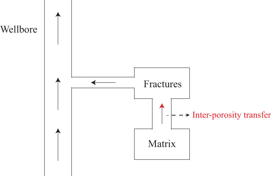
The flow process of the gas.
In addition, some assumptions are made to assist in the development of the model.
The formation is an isotropic cylinder, and the thickness of the formation remains unchanged.
There is a gas well with constant production at the center of the formation.
The formation fluid is only gas, and the flow satisfies Darcy’s law.
The capillary force and gravity are negligible.
2.2 Mathematical model
2.2.1 Quasi-steady state model
After the physical model is established, the formula of inter-porosity transfer rate can be derived by the mathematical model. Initially, the quasi-steady state model is studied. For the specific meanings of mathematical symbols, please see Nomenclature.
The continuity equation should be satisfied for the gas in the matrix and fractures, which is shown as follows:
where subscript f represents the fracture system and subscript m represents the matrix system. q represents the inter-porosity transfer rate.
The state equation of gas is as follows:
Pseudo-pressure is introduced instead of pressure.
According to the previous study, the matrix permeability is much lower than the fracture permeability. Therefore, the variation of fluid mass caused by seepage conduction in the matrix system is negligible compared with the inter-porosity transfer term and the elastic term. So
The introduction of dimensionless parameters can simplify the mathematical formula. It can better present the characteristics of fast and convenient analytical solutions [26].
The dimensionless parameters used in this work are defined as follows:
After the dimensionless process, Eqs. (5) and (6) can be converted to
Laplace transform is performed on Eq. (14). Then, Eq. (15) can be obtained.
where
From Eq. (15), we can obtain Eqs. (16) and (17) as follows:
where
The general solution of Eq. (17) is
Since the gas well is produced at a constant production rate, the internal boundary conditions can be obtained as follows:
There are three kinds of external boundary conditions. Eqs. (20)–(22) represent the infinite gas reservoir boundary, closed boundary, and constant pressure boundary, respectively.
Therefore,
In the quasi-steady state model, the inter-porosity transfer rate is related to the following factors: (i) the pressure difference between matrix and fractures; (ii) gas viscosity; (iii) shape factor; (iv) permeability of matrix; and (v) gas density.
The formula is as follows:
Using Eqs. (4), (7), (8), and (11) to transform Eq. (23), we can obtain
Laplace transform is performed on Eq. (24).
In the above discussion, the relationship between
So
where
From Eq. (27), we can obtain the inter-porosity transfer rate in the Laplace domain. After that, Stehfest inversion [27] is employed to convert the inter-porosity transfer rate into physical domain.
2.2.2 Unsteady state model
The mathematical model of the unsteady state model is still composed of the seepage equation of fracture and the seepage equation of matrix. The equation of the fracture is the same as that of the quasi-steady state model. But the equation of matrix is different between the quasi-steady state model and the unsteady state model.
As mentioned above, the unsteady state models can be divided into spherical, plate, and cylindrical models. We will study the spherical model in this section. The formula derivation process for the other two models is in Appendix A.
As shown in Figure 3(a), each sphere has the same shape, and the radius is
The inter-porosity transfer rate can be expressed as follows:
Define two dimensionless parameters here:
For fracture system,
The dimensionless equation of the spherical model is as follows:
where
The Laplace transform is performed on Eq. (30).
It can be obtained after solving Eq. (31):
If the dimensionless transform and Laplace transform are performed on Eq. (29), then we can obtain
This is the formula of inter-porosity transfer rate in the Laplace domain. As discussed in Section 2.2.1, we need to research the relationship of
According to Eq. (32), we can obtain
Substituting Eq. (34) into the first term of Eq. (31), we have
where
Based on the above discussion, we can obtain
2.3 Summary of mathematical model
The inter-porosity transfer rate of both quasi-steady state model and unsteady state models can be calculated by Eq. (37). It is just that f(s) has different forms. Table 1 shows the forms of f(s) for different models.
The
| Type of model |
|
|---|---|
| Steady state |
|
| Spherical model |
|
| Plate model |
|
| Cylindrical model |
|
The solution steps are as follows: first, calculate the fracture pseudo-pressure
2.4 The solution of producing degree of matrix
As mentioned in Section 1, the producing degree of matrix is defined as the ratio of gas from the matrix to total gas production. It can reflect the degree of gas development in the matrix. The formula is as follows:
where C m is the producing degree of matrix and Q m is the gas from matrix. Q t is the total gas production.
The radius of the gas reservoir is r e, and the radius of the wellbore is r w. In order to calculate the producing degree of matrix, the gas reservoir is divided into n rings, which are shown in Figure 5. The ring width is dr. As discussed above, the inter-porosity transfer rate of each ring can be calculated. The sum of n rings is the total amount of gas from the matrix entering the fractures. The further formula to calculate the producing degree of matrix is as follows:

Schematic diagram of gas reservoir division.
In order to present the work clearer, the specific steps are presented by a flowchart, which is shown in Figure 6.

The specific steps of the work.
3 Typical curves analysis
The main object of this article is to study the inter-porosity transfer rate and producing degree of matrix when gas reservoirs are producing. The typical curves are an appropriate tool to identify the flow stage and characteristics involved in the problem being investigated [28]. Hence, we plot the typical curves of inter-porosity transfer rate and producing degree of matrix in this section.
3.1 Typical curves of inter-porosity transfer rate
When storage ratio ω = 0.12, inter-porosity flow factor λ = 10−6, r eD = 1,000 (r eD = r e/r w), and r D = 1, under a closed boundary, plot the typical curves of inter-porosity transfer rate.
Here, r D is equal to 1, which means the inter-porosity transfer rate is near the wellbore. When r d takes different values, the inter-porosity transfer rate at different positions can be calculated.
Figure 7(a) represents the quasi-steady state model, and Figure 7(b) represents the three kinds of unsteady state models.

Inter-porosity transfer rate of quasi-steady state model and unsteady state models: (a) quasi-steady state model and (b) unsteady state models.
As shown in Figure 7(a), the typical curve of inter-porosity transfer rate near the wellbore can be divided into three stages.
Stage I is the straight line stage. At this time, the gas reservoir starts to produce. The gas production is mainly supplied by the gas originally held in the wellbore. Affected by this, the inter-porosity transfer rate curve is a straight line.
Stage II is the fracture radial flow stage and the transition stage. In this stage, the pressure in the fracture system decreases, while the pressure in the matrix system is almost constant. The pressure difference between the matrix system and the fracture system increases. Therefore, the inter-porosity transfer rate gradually increases. After that, the gas reservoir goes to the transition stage. With continuous production, the pressure in the matrix system decreases gradually. The pressure difference becomes smaller, so the inter-porosity transfer rate begins to decrease.
Stage III is the total radial flow stage. At this stage, the pressure has propagated to the external boundary. The inter-porosity transfer rate stays constant.
As shown in Figure 7(b), the inter-porosity transfer rate of unsteady state models is different from the quasi-steady state model. In the unsteady state models, the inter-porosity transfer between matrix and fractures is transient and fast, which is regarded as an unsteady process. As can be seen in Figure 7(b), the straight line stage of unsteady steady models ends earlier. The biggest difference between the quasi-steady state model and the unsteady state model happens in stage II. In the unsteady state models, the inter-porosity transfer rate first reaches its peak in a short time and then gradually decreases, which is contrary to the quasi-steady state model. The typical curves are the same in stage III between the quasi-steady state model and unsteady state models.
Comparing the three kinds of unsteady models, it can be found that their inter-porosity transfer rate is slightly different in stage II. The inter-porosity transfer rate of the spherical model is the largest. The second largest is the cylindrical model. The inter-porosity transfer rate of plate model is smaller than that of spherical model and cylindrical model.
3.2 Typical curves of producing degree of matrix
When ω = 0.12, λ = 10−6, and r eD = 1,000, plot the typical curves of producing degree of matrix. Figure 8(a) represents the producing degree of matrix for the quasi-steady state model. Since the difference in transfer rate between the three unsteady models is extremely tiny, only the spherical model is selected here for comparison with the quasi-steady model. Figure 8(b) represents the comparison between the quasi-steady state model and the spherical model.

Producing degree of matrix for quasi-steady state model and unsteady state models. (a) Quasi-steady state model. (b) A comparison between quasi-steady state model and spherical model.
Figure 8(a) shows that the typical curve can be divided into three stages. When t D from 0 to 103, the producing degree of matrix increases extremely slowly. When t D from 103 to 106, it increases rapidly to 0.7. After that, it remains at 0.7. It indicates that the total amount of gas from matrix entering fractures remains invariable when t D > 106. We can also draw the conclusion that 70% of the total production comes from the gas in the matrix.
It can be seen from Figure 8(b) that the variation trend of the typical curve in the unsteady state model is the same as that in the quasi-steady state model. But the typical curve of the unsteady state model begins to increase rapidly when t D = 102. It indicates that the transfer occurs earlier in the unsteady model. The growth rate of producing degree of matrix is less than that of the quasi-steady state model, so it reaches the constant state later.
3.3 Model validation
In order to verify the accuracy of our model, a comparison between our model and the model of Hassanzadeh is presented here. Hassanzadeh et al. [29] studied the shape factor in dual-porosity systems under a constant rate at the wellbore. He calculated the matrix–fracture transfer rate in infinite boundary based on their research findings. In our model, we consider the effect of wellbore constant and skin factor. But when r eD is large enough, the effects of those become small. In this situation, our model is similar to the model of Hassanzadeh. Hence, we make ω = 0.03, λ = 10−6, and r D = 1,000 and plot the typical curve of inter-porosity transfer rate in the plate model. The parameters that we choose are the same as those in Hassanzadeh’s model. The comparison result is shown in Figure 9. It can be seen that the calculation results of the two models match well. This comparison indicates our model is accurate.
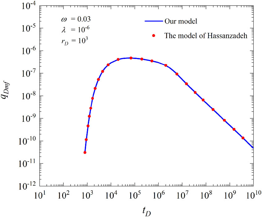
The comparison result between our model and Hassanzadeh’s model.
4 Sensitivity analysis
Gas reservoir radius r eD, storage ratio ω, and inter-porosity flow factor λ are all key parameters for the inter-porosity transfer rate and producing degree of matrix. Different parameters will greatly change the curve’s shape. In this section, we take quasi-steady state model as an example to analyze the influence of key parameters.
4.1 The influence of gas reservoir radius
As discussed above, the inter-porosity transfer rate at various positions is different. When ω = 0.12, λ = 10−6, gas reservoir radius r eD = 1,000, and making r D = 1, 10, 100, and 1,000, under a closed boundary, plot the transfer rate curves, which are shown in Figure 10. It is found that the inter-porosity transfer rate near the wellbore is the largest. The further away from the wellbore, the smaller the inter-porosity transfer rate is. But when pressure propagates to the external boundary, the inter-porosity transfer rate is equal in the whole gas reservoir.

Typical curves of inter-porosity transfer rate at different positions of gas reservoirs.
Then, we take the inter-porosity transfer rate near the wellbore as an example to study the influence of gas reservoir radius. When ω = 0.12, λ = 10−6, r D = 1, making r eD = 1,000, 1,500, and 2,000, plot the transfer rate curves, which are shown in Figure 11. It can be seen that the gas reservoir radius has no influence on the inter-porosity transfer rate in the initial and middle periods. In the late period, when the gas reservoir radius increases, the inter-porosity transfer rate becomes smaller. It can also be found that the typical curves become horizontal line later. It is because the pressure propagates to the external boundary later when the gas reservoir radius increases.

The influence of gas reservoir radius on inter-porosity transfer rate near the wellbore.
4.2 The influence of storage ratio
When λ = 10−6, r D = 1, r eD = 1,000 making ω = 0.03, 0.06 and 0.12, plot the typical curves. Figure 12 shows the influence of storage ratio on inter-porosity transfer rate. When ω becomes larger, the inter-porosity transfer rate decreases, and the curves move down. Figure 13 shows the influence of storage ratio on producing degree of matrix. When ω becomes larger, the producing degree of matrix decreases. Meanwhile, it becomes stable later. The above situation indicates that the inter-porosity transfer between the matrix and fractures will occur later when ω becomes larger. Besides, the total amount of inter-porosity transfer will decrease, which leads the gas in the matrix to be less developed.

The influence of ω on inter-porosity transfer rate.

The influence of ω on producing degree of matrix.
4.3 The influence of inter-porosity flow factor
When ω = 0.12, r
D = 1, r
eD = 1,000, and making λ = 10−4, 10−5, and 10−6, plot the typical curves. Figure 14 shows the influence of λ on the inter-porosity transfer rate. Before the curves become horizontal, when λ becomes smaller, the inter-porosity transfer rate decreases. But when t
D

The influence of λ on inter-porosity transfer rate.

The influence of λ on producing degree of matrix.
5 Case analysis
Shapingchang gas field is situated in Sichuan, western China. The main gas reservoirs in Shapingchang are carboniferous carbonate gas reservoirs. These gas reservoirs are fractured-porous gas reservoirs with medium to low porosity and permeability. Well X6 and Well Y6 in the Shapingchang gas field are exemplified in this article.
The production characteristics curves of Well X6 and Well Y6 are plotted in Figures 16 and 17. The blue curve represents the gas production per month. The red curve represents the cumulative gas production since the well was opened. The production characteristics of X6 and Y6 are analyzed through the curves.

The production characteristics curve of Well X6.

The production characteristics curve of Well Y6.
According to the logging data, it is found that the fractures are relatively developed in Well X6, with 192 effective fractures in total. The average fracture density is 5.5 pieces/m, the average porosity is 6.23%, and the storage ratio is 0.11. According to Figure 16, it is found that the initial production of Well X6 is very high, about 1,500
The number of fractures in Well Y6 is small, and there are 30 effective fractures in total. Its average porosity is 5.9%, and the storage ratio is 0.04. According to Figure 17, it is found that the initial production of Well Y6 is relatively low, about 780
According to the typical curve of producing degree of matrix in Section 3, the producing degree of matrix is very small in the early period. It indicates that the gas production mainly comes from fractures. Because the fracture conductivity is strong, the initial gas production is high. However, the gas reserve in the fractures is small. Besides, the inter-porosity transfer rate is also low in the early period. Therefore, the gas supply from the matrix to fractures is very slow, which results in a rapid reduction in gas production. During the mid-late period, the producing degree of matrix is large, demonstrating that the matrix provides the majority of the gas production. The gas well maintains a long time of low-speed production. The actual production characteristics are in line with the previous discussion.
The storage ratio of X6 is large, so the inter-porosity transfer rate is relatively small. Therefore, the gas supplied by the matrix is relatively low, which leads to gas production decreasing rapidly. The storage ratio of Y6 is small, indicating that the inter-porosity transfer rate is relatively large. So the gas supplied by the matrix is relatively high, which leads to gas production decreasing slowly. The actual production characteristics are also consistent with the sensitivity analysis.
6 Summary and conclusions
The inter-porosity transfer rate and producing degree of matrix are very essential research topics for the development of fractured-porous gas reservoirs. In this article, we establish a practical analytical solution for calculating the inter-porosity transfer rate and producing degree of matrix. Some conclusions are summarized as follows:
We establish a concise formula for the inter-porosity transfer rate. By adjusting f(s), the formula is applicable to the quasi-steady state model and unsteady state model. Then, by summing the inter-porosity transfer rate at different positions of the gas reservoir, we obtain the solution for the producing degree of matrix.
In the initial period of production, the producing degree of matrix is close to zero, indicating that there is almost no inter-porosity transfer. Then, the transfer rate begins to increase. In the late period, the producing degree of matrix is large, which means that most of the gas production comes from the matrix.
The inter-porosity transfer rate near the wellbore is the largest. The further away from the wellbore, the smaller the inter-porosity transfer rate. In comparison to the quasi-steady state model, the inter-porosity transfer occurs earlier in the unsteady model. But when pressure propagates to the external boundary, the inter-porosity transfer rate is equal between the quasi-steady and unsteady models.
The inter-porosity transfer can be significantly influenced by the gas reservoir radius, storage ratio (ω), and inter-porosity flow factor λ. When ω increases, the inter-porosity transfer rate and producing degree of matrix both decrease. Meanwhile, the transfer occurs later. When λ increases, the transfer occurs earlier. But it does not influence the total amount of inter-porosity transfer. The gas reservoir radius mainly influences the late period of the inter-porosity transfer.
Two fractured-porous gas reservoirs from Shapingchang are analyzed. The producing characteristics can be explained by our findings.
The model in this article is developed based on the dual-porosity approach. The gas in the matrix that directly flows into the wellbore is negligible. However, the matrix permeability may be large in some fractured-porous gas reservoirs. In this case, our model may be inaccurate.
In this study, the fluid in the formation is single phase. In some fractured-porous gas reservoirs, there may be water in the late period during production. Hence, the fluid in the formation is two phase. Our model is not applicable to the two-phase flow. In view of this, we will develop the two-phase flow model in the future.
Acknowledgments
The authors gratefully acknowledge the funding support from the National Science and Technology Major Project (Grant No. 2017ZX05009005-002).
-
Funding information: The funding support was granted from the National Science and Technology Major Project (Grant No. 2017ZX05009005-002).
-
Author contributions: All authors have accepted responsibility for the entire content of this manuscript and approved its submission.
-
Conflict of interest: The authors state no conflict of interest.
-
Data availability statement: The datasets generated during and/or analysed during the current study are available from the corresponding author on reasonable request.
Appendix A
A1 The inter-porosity transfer rate of cylindrical model
The shape of each cylinder is the same, and the radius is
The inter-porosity transfer rate can be expressed by the following formula:
The dimensionless seepage equation is as follows:
where
Laplace transform is performed on the second to the fourth terms of Eq. (A3).
The solution of Eq. (A4) is
After dimensionless and Laplace transform, Eq. (A2)can be written as follows:
Laplace transform is performed on the first term of Eq. (A3).
According to Eq. (A5), we can obtain
Substituting Eq. (A8) into Eq. (A7), we obtain
where
Combining Eqs. (A6), (A7), and (A9), we can obtain
A2 The inter-porosity transfer rate of plate model
Each plate has the same shape, and the thickness is
The inter-porosity transfer rate can be expressed by the following formula:
After dimensionless and Laplace transform, Eq. (A12) can be written as follows:
The seepage equation after Laplace transformation is as follows:
where
From the second to the fourth terms of Eq. (A14), we can obtain
Then, substitute Eq. (A15) into the first term of Eq. (14).
where
Combining Eqs. (A13), (A14), and (A16), the inter-porosity transfer rate of plate model is
References
[1] Wei C, Cheng S, Wang Y, Shi W, Li J, Zhang J, et al. Practical pressure-transient analysis solutions for a well intercepted by finite conductivity vertical fracture in naturally fractured reservoirs. J Pet Sci Eng. 2021;204:108768.10.1016/j.petrol.2021.108768Search in Google Scholar
[2] Jia A, Yan H, Guo J, He D, Cheng L, Jia C. Development characteristics for different types of carbonate gas reservoirs. Acta Pet Sin. 2013;34(5):914–23.Search in Google Scholar
[3] Ranjbar E, Hassanzadeh H. Matrix-fracture transfer shape factor for modeling flow of a compressible fluid in dual-porosity media. Adv Water Resour. 2011;34(5):627–39.10.1016/j.advwatres.2011.02.012Search in Google Scholar
[4] Sun Q, Zhang N, Fadlelmula M, Wang Y. Structural regeneration of fracture-vug network in naturally fractured vuggy reservoirs. J Pet Sci Eng. 2018;165:28–41.10.1016/j.petrol.2017.11.030Search in Google Scholar
[5] Ranjbar E, Hassanzadeh H, Chen Z. Effect of fracture pressure depletion regimes on the dual-porosity shape factor for flow of compressible fluids in fractured porous media. Adv Water Resour. 2011;34(12):1681–93.10.1016/j.advwatres.2011.09.010Search in Google Scholar
[6] Jiao C, Hu Y, Xu X, Lu X, Shen W, Hu X. Study on the effects of fracture on permeability with pore-fracture network model. Energy Explor Explo. 2018;36(6):1556–65.10.1177/0144598718777115Search in Google Scholar
[7] Wang W, Yao J, Li Y, Lv A. Research on carbonate reservoir interwell connectivity based on a modified diffusivity filter model. Open Phys. 2017;15(1):306–12.10.1515/phys-2017-0034Search in Google Scholar
[8] Cao R, Xu Z, Cheng L, Peng Y, Wang Y, Guo Z. Study of single phase mass transfer between matrix and fracture in tight oil reservoirs. Geofluids. 2019;2019:1038412.10.1155/2019/1038412Search in Google Scholar
[9] Chu H, Liao X, Chen Z, Zhao X, Liu W, Zou J. Pressure transient analysis in fractured reservoirs with poorly connected fractures. J Nat Gas Sci Eng. 2019;67:30–42.10.1016/j.jngse.2019.04.015Search in Google Scholar
[10] Jia YL, Wang BC, Nie RS, Wang DL. New transient-flow modelling of a multiple-fractured horizontal well. J Geophys Eng. 2014;11(1):015013.10.1088/1742-2132/11/1/015013Search in Google Scholar
[11] Wei C, Cheng S, Tu K, An X, Qu D, Zeng F, et al. A hybrid analytic solution for a well with a finite-conductivity vertical fracture. J Pet Sci Eng. 2020;188:106900.10.1016/j.petrol.2019.106900Search in Google Scholar
[12] Wan YZ, Liu YW, Chen FF, Wu NY, Hu GW. Numerical well test model for caved carbonate reservoirs and its application in Tarim Basin, China. J Pet Sci Eng. 2018;161:611–24.10.1016/j.petrol.2017.12.013Search in Google Scholar
[13] Barenblatt GI, Zheltov YP, Kochina IN. Basic concepts in the theory of seepage of homogeneous liquids in fissured rocks. J Appl Math. 1960;24(5):5–1303.10.1016/0021-8928(60)90107-6Search in Google Scholar
[14] Warren JE, Root PJ. The behavior of naturally fractured reservoirs abstract. Soc Pet Eng J. 1963;3(3):245–55.10.2118/426-PASearch in Google Scholar
[15] Kazemi H. Pressure transient analysis of naturally fractured reservoirs with uniform fracture distribution. Soc Pet Eng J. 1969;9(4):451–62.10.2118/2156-ASearch in Google Scholar
[16] Deswaano A. Analytic solutions for determining naturally fractured reservoir properties by well testing. Soc Pet Eng J. 1976;16(3):117–22.10.2118/5346-PASearch in Google Scholar
[17] Zimmerman RW, Chen G, Hadgu T, Bodvarsson GS. A numerical dual-porosity model with semianalytical treatment of fracture matrix flow. Water Resour Res. 1993;29(7):2127–37.10.1029/93WR00749Search in Google Scholar
[18] Lim KT, Aziz K. Matrix-fracture transfer shape factors for dual-porosity simulators. J Pet Sci Eng. 1995;13(3–4):169–78.10.1016/0920-4105(95)00010-FSearch in Google Scholar
[19] Zhou D, Ge J, Li Y, Cai Y. Establishment of interporosity flow function of complex fractured reservoir. Oil Gas Rec Tec. 2000;7(2):30–2.Search in Google Scholar
[20] Zheng H, Shi AF, Liu ZF, Wang XH. A dual-porosity model considering the displacement effect for incompressible two-phase flow. Int J Numer Anal Methods Geomech. 2020;44(5):691–704.10.1002/nag.3037Search in Google Scholar
[21] Fansheng B, Shusheng G, Wei X, Hui X. Fluid cross flow law in fractured-porous dual media reservoir. J Liaoning Tech Univ. 2008;27(5):677–9.Search in Google Scholar
[22] Lian PQ, Cheng LS, Li LL, Li Z. The variation law of storativity ratio and interporosity transfer coefficient in fractured reservoirs. Eng Mech. 2011;28(9):240–4.Search in Google Scholar
[23] Xiangguo LU, Jianchong GAO, Xin HE, Wei Yanchang SU, Xiuling PEI. Experimental study of internal channeling law of intra-layer heterogeneous reservoir: A case study of Lamadian Oilfield in Daqing. Editor Dep Pet Geol Recovery Efficiency. 2023;29(5):118–25.Search in Google Scholar
[24] Kumar S, Mohan B. A study of multi-soliton solutions, breather, lumps, and their interactions for Kadomtsev-Petviashvili equation with variable time coefficient using Hirota method. Phys Scr. 2021;96(12):125255.10.1088/1402-4896/ac3879Search in Google Scholar
[25] Kumar S, Mohan B, Kumar A. Generalized fifth-order nonlinear evolution equation for the Sawada-Kotera, Lax, and Caudrey-Dodd-Gibbon equations in plasma physics: Painlevé analysis and multi-soliton solutions. Phys Scr. 2022;97(3):035201.10.1088/1402-4896/ac4f9dSearch in Google Scholar
[26] Kumar S, Rani S. Lie symmetry reductions and dynamics of soliton solutions of (2 + 1)-dimensional Pavlov equation. Pramana-J Phys. 2020;94(1):116.10.1007/s12043-020-01987-wSearch in Google Scholar
[27] Stehfest H. Algorithm 368: Numerical inversion of Laplace transforms [D5]. Commun Acm. 1970;13(1):47–9.10.1145/361953.361969Search in Google Scholar
[28] Dejam M, Hassanzadeh H, Chen Z. Semi-analytical solution for pressure transient analysis of a hydraulically fractured vertical well in a bounded dual-porosity reservoir . J Hydrol. 2018;565:289–301.10.1016/j.jhydrol.2018.08.020Search in Google Scholar
[29] Hassanzadeh H, Pooladi-Darvish M, Atabay S. Shape factor in the drawdown solution for well testing of dual-porosity systems. Adv Water Resour. 2009;32(11):1652–63.10.1016/j.advwatres.2009.08.006Search in Google Scholar
© 2023 the author(s), published by De Gruyter
This work is licensed under the Creative Commons Attribution 4.0 International License.
Articles in the same Issue
- Regular Articles
- Dynamic properties of the attachment oscillator arising in the nanophysics
- Parametric simulation of stagnation point flow of motile microorganism hybrid nanofluid across a circular cylinder with sinusoidal radius
- Fractal-fractional advection–diffusion–reaction equations by Ritz approximation approach
- Behaviour and onset of low-dimensional chaos with a periodically varying loss in single-mode homogeneously broadened laser
- Ammonia gas-sensing behavior of uniform nanostructured PPy film prepared by simple-straightforward in situ chemical vapor oxidation
- Analysis of the working mechanism and detection sensitivity of a flash detector
- Flat and bent branes with inner structure in two-field mimetic gravity
- Heat transfer analysis of the MHD stagnation-point flow of third-grade fluid over a porous sheet with thermal radiation effect: An algorithmic approach
- Weighted survival functional entropy and its properties
- Bioconvection effect in the Carreau nanofluid with Cattaneo–Christov heat flux using stagnation point flow in the entropy generation: Micromachines level study
- Study on the impulse mechanism of optical films formed by laser plasma shock waves
- Analysis of sweeping jet and film composite cooling using the decoupled model
- Research on the influence of trapezoidal magnetization of bonded magnetic ring on cogging torque
- Tripartite entanglement and entanglement transfer in a hybrid cavity magnomechanical system
- Compounded Bell-G class of statistical models with applications to COVID-19 and actuarial data
- Degradation of Vibrio cholerae from drinking water by the underwater capillary discharge
- Multiple Lie symmetry solutions for effects of viscous on magnetohydrodynamic flow and heat transfer in non-Newtonian thin film
- Thermal characterization of heat source (sink) on hybridized (Cu–Ag/EG) nanofluid flow via solid stretchable sheet
- Optimizing condition monitoring of ball bearings: An integrated approach using decision tree and extreme learning machine for effective decision-making
- Study on the inter-porosity transfer rate and producing degree of matrix in fractured-porous gas reservoirs
- Interstellar radiation as a Maxwell field: Improved numerical scheme and application to the spectral energy density
- Numerical study of hybridized Williamson nanofluid flow with TC4 and Nichrome over an extending surface
- Controlling the physical field using the shape function technique
- Significance of heat and mass transport in peristaltic flow of Jeffrey material subject to chemical reaction and radiation phenomenon through a tapered channel
- Complex dynamics of a sub-quadratic Lorenz-like system
- Stability control in a helicoidal spin–orbit-coupled open Bose–Bose mixture
- Research on WPD and DBSCAN-L-ISOMAP for circuit fault feature extraction
- Simulation for formation process of atomic orbitals by the finite difference time domain method based on the eight-element Dirac equation
- A modified power-law model: Properties, estimation, and applications
- Bayesian and non-Bayesian estimation of dynamic cumulative residual Tsallis entropy for moment exponential distribution under progressive censored type II
- Computational analysis and biomechanical study of Oldroyd-B fluid with homogeneous and heterogeneous reactions through a vertical non-uniform channel
- Predictability of machine learning framework in cross-section data
- Chaotic characteristics and mixing performance of pseudoplastic fluids in a stirred tank
- Isomorphic shut form valuation for quantum field theory and biological population models
- Vibration sensitivity minimization of an ultra-stable optical reference cavity based on orthogonal experimental design
- Effect of dysprosium on the radiation-shielding features of SiO2–PbO–B2O3 glasses
- Asymptotic formulations of anti-plane problems in pre-stressed compressible elastic laminates
- A study on soliton, lump solutions to a generalized (3+1)-dimensional Hirota--Satsuma--Ito equation
- Tangential electrostatic field at metal surfaces
- Bioconvective gyrotactic microorganisms in third-grade nanofluid flow over a Riga surface with stratification: An approach to entropy minimization
- Infrared spectroscopy for ageing assessment of insulating oils via dielectric loss factor and interfacial tension
- Influence of cationic surfactants on the growth of gypsum crystals
- Study on instability mechanism of KCl/PHPA drilling waste fluid
- Analytical solutions of the extended Kadomtsev–Petviashvili equation in nonlinear media
- A novel compact highly sensitive non-invasive microwave antenna sensor for blood glucose monitoring
- Inspection of Couette and pressure-driven Poiseuille entropy-optimized dissipated flow in a suction/injection horizontal channel: Analytical solutions
- Conserved vectors and solutions of the two-dimensional potential KP equation
- The reciprocal linear effect, a new optical effect of the Sagnac type
- Optimal interatomic potentials using modified method of least squares: Optimal form of interatomic potentials
- The soliton solutions for stochastic Calogero–Bogoyavlenskii Schiff equation in plasma physics/fluid mechanics
- Research on absolute ranging technology of resampling phase comparison method based on FMCW
- Analysis of Cu and Zn contents in aluminum alloys by femtosecond laser-ablation spark-induced breakdown spectroscopy
- Nonsequential double ionization channels control of CO2 molecules with counter-rotating two-color circularly polarized laser field by laser wavelength
- Fractional-order modeling: Analysis of foam drainage and Fisher's equations
- Thermo-solutal Marangoni convective Darcy-Forchheimer bio-hybrid nanofluid flow over a permeable disk with activation energy: Analysis of interfacial nanolayer thickness
- Investigation on topology-optimized compressor piston by metal additive manufacturing technique: Analytical and numeric computational modeling using finite element analysis in ANSYS
- Breast cancer segmentation using a hybrid AttendSeg architecture combined with a gravitational clustering optimization algorithm using mathematical modelling
- On the localized and periodic solutions to the time-fractional Klein-Gordan equations: Optimal additive function method and new iterative method
- 3D thin-film nanofluid flow with heat transfer on an inclined disc by using HWCM
- Numerical study of static pressure on the sonochemistry characteristics of the gas bubble under acoustic excitation
- Optimal auxiliary function method for analyzing nonlinear system of coupled Schrödinger–KdV equation with Caputo operator
- Analysis of magnetized micropolar fluid subjected to generalized heat-mass transfer theories
- Does the Mott problem extend to Geiger counters?
- Stability analysis, phase plane analysis, and isolated soliton solution to the LGH equation in mathematical physics
- Effects of Joule heating and reaction mechanisms on couple stress fluid flow with peristalsis in the presence of a porous material through an inclined channel
- Bayesian and E-Bayesian estimation based on constant-stress partially accelerated life testing for inverted Topp–Leone distribution
- Dynamical and physical characteristics of soliton solutions to the (2+1)-dimensional Konopelchenko–Dubrovsky system
- Study of fractional variable order COVID-19 environmental transformation model
- Sisko nanofluid flow through exponential stretching sheet with swimming of motile gyrotactic microorganisms: An application to nanoengineering
- Influence of the regularization scheme in the QCD phase diagram in the PNJL model
- Fixed-point theory and numerical analysis of an epidemic model with fractional calculus: Exploring dynamical behavior
- Computational analysis of reconstructing current and sag of three-phase overhead line based on the TMR sensor array
- Investigation of tripled sine-Gordon equation: Localized modes in multi-stacked long Josephson junctions
- High-sensitivity on-chip temperature sensor based on cascaded microring resonators
- Pathological study on uncertain numbers and proposed solutions for discrete fuzzy fractional order calculus
- Bifurcation, chaotic behavior, and traveling wave solution of stochastic coupled Konno–Oono equation with multiplicative noise in the Stratonovich sense
- Thermal radiation and heat generation on three-dimensional Casson fluid motion via porous stretching surface with variable thermal conductivity
- Numerical simulation and analysis of Airy's-type equation
- A homotopy perturbation method with Elzaki transformation for solving the fractional Biswas–Milovic model
- Heat transfer performance of magnetohydrodynamic multiphase nanofluid flow of Cu–Al2O3/H2O over a stretching cylinder
- ΛCDM and the principle of equivalence
- Axisymmetric stagnation-point flow of non-Newtonian nanomaterial and heat transport over a lubricated surface: Hybrid homotopy analysis method simulations
- HAM simulation for bioconvective magnetohydrodynamic flow of Walters-B fluid containing nanoparticles and microorganisms past a stretching sheet with velocity slip and convective conditions
- Coupled heat and mass transfer mathematical study for lubricated non-Newtonian nanomaterial conveying oblique stagnation point flow: A comparison of viscous and viscoelastic nanofluid model
- Power Topp–Leone exponential negative family of distributions with numerical illustrations to engineering and biological data
- Extracting solitary solutions of the nonlinear Kaup–Kupershmidt (KK) equation by analytical method
- A case study on the environmental and economic impact of photovoltaic systems in wastewater treatment plants
- Application of IoT network for marine wildlife surveillance
- Non-similar modeling and numerical simulations of microploar hybrid nanofluid adjacent to isothermal sphere
- Joint optimization of two-dimensional warranty period and maintenance strategy considering availability and cost constraints
- Numerical investigation of the flow characteristics involving dissipation and slip effects in a convectively nanofluid within a porous medium
- Spectral uncertainty analysis of grassland and its camouflage materials based on land-based hyperspectral images
- Application of low-altitude wind shear recognition algorithm and laser wind radar in aviation meteorological services
- Investigation of different structures of screw extruders on the flow in direct ink writing SiC slurry based on LBM
- Harmonic current suppression method of virtual DC motor based on fuzzy sliding mode
- Micropolar flow and heat transfer within a permeable channel using the successive linearization method
- Different lump k-soliton solutions to (2+1)-dimensional KdV system using Hirota binary Bell polynomials
- Investigation of nanomaterials in flow of non-Newtonian liquid toward a stretchable surface
- Weak beat frequency extraction method for photon Doppler signal with low signal-to-noise ratio
- Electrokinetic energy conversion of nanofluids in porous microtubes with Green’s function
- Examining the role of activation energy and convective boundary conditions in nanofluid behavior of Couette-Poiseuille flow
- Review Article
- Effects of stretching on phase transformation of PVDF and its copolymers: A review
- Special Issue on Transport phenomena and thermal analysis in micro/nano-scale structure surfaces - Part IV
- Prediction and monitoring model for farmland environmental system using soil sensor and neural network algorithm
- Special Issue on Advanced Topics on the Modelling and Assessment of Complicated Physical Phenomena - Part III
- Some standard and nonstandard finite difference schemes for a reaction–diffusion–chemotaxis model
- Special Issue on Advanced Energy Materials - Part II
- Rapid productivity prediction method for frac hits affected wells based on gas reservoir numerical simulation and probability method
- Special Issue on Novel Numerical and Analytical Techniques for Fractional Nonlinear Schrodinger Type - Part III
- Adomian decomposition method for solution of fourteenth order boundary value problems
- New soliton solutions of modified (3+1)-D Wazwaz–Benjamin–Bona–Mahony and (2+1)-D cubic Klein–Gordon equations using first integral method
- On traveling wave solutions to Manakov model with variable coefficients
- Rational approximation for solving Fredholm integro-differential equations by new algorithm
- Special Issue on Predicting pattern alterations in nature - Part I
- Modeling the monkeypox infection using the Mittag–Leffler kernel
- Spectral analysis of variable-order multi-terms fractional differential equations
- Special Issue on Nanomaterial utilization and structural optimization - Part I
- Heat treatment and tensile test of 3D-printed parts manufactured at different build orientations