Multiple Lie symmetry solutions for effects of viscous on magnetohydrodynamic flow and heat transfer in non-Newtonian thin film
-
Muhammad Safdar
 ,
Safia Taj
,
Safia Taj

Abstract
Numerous flow and heat transfer studies have relied on the construction of similarity transformations which map the nonlinear partial differential equations (PDEs) describing the flow and heat transfer, to ordinary differential equations (ODEs). For these reduced equations, one finds multiple analytic and approximate solution procedures as compared to the flow PDEs. Here, we aim at constructing multiple classes of similarity transformations that are different from those already existing in the literature. We adopt the Lie symmetry method to derive these new similarity transformations which reveal new classes of ODEs corresponding to flow equations when applied to them. With these multiple classes of similarity transformations, one finds multiple reductions in the flow PDEs to ODEs. On solving these ODEs analytically or numerically, we obtain different kinds of flow and heat transfer patterns that help in determining optimized solutions in accordance with the physical requirements of a problem. For the said purpose, we derive Lie point symmetries for the magnetohydrodynamic Casson fluid flow and heat transfer in a thin film on an unsteady stretching sheet with viscous dissipation. Linear combinations of these Lie symmetries that are again the Lie symmetries of the flow model are employed here to construct new similarity transformations. We derive multiple Lie similarity transformations through the proposed procedure which lead us to more than one class of reduced ODEs obtained by applying the deduced transformations. We analyze the flow and heat transfer by deriving analytic solutions for the obtained classes of systems of ODEs using the homotopy analysis method. Magnetic parameters and viscous dissipation influences on the flow and heat transports are investigated and presented in graphical and tabulated formats.
1 Introduction
In a thin liquid film on an unsteady stretching surface, fluid flow and transfer of heat remained a field that received an enormous amount of attention over the past few decades [1,2,3,4,5,6,7,8,9,10,11,12,13]. These studies have been conducted by researchers working in different areas, e.g., engineering, pharmaceutical, physical sciences, and biology. The contributions signify the importance of fluid flows and heat transfers in thin films. To mention a few applications of fluid flows and heat transfers in thin films, one may consider coating wires as well as fibers, transpiration cooling, processing of food, reactor fluidization, and heat exchangers. Therefore, these problems are studied extensively under different physical conditions to acquire the optimum flow and heat transfer needed for a specific quality of a product. These studies are conducted experimentally as well as theoretically. For theoretical investigations, an approach that is adopted in many attempts is the conversion of the flow models that are genuinely non-linear partial differential equations (PDEs), to ordinary differential equations (ODEs). Similarity transformations enable such a reduction. Hence, through the construction of such similarity transformation, new solvable classes of the flow and heat transfer problems are revealed [14,15,16,17]. Reduction of PDEs defining these transports to ODEs eases derivations of solutions using approximate or analytic methods [18,19]. Because there are several well-established approximate and analytic solution schemes that are available for ODEs as compared to PDEs. Similarity transformations are invertible maps, i.e., they transform the flow PDEs to ODEs that are solved analytically or numerically and then these solutions can be inverted to obtain solutions for the flow PDEs. There exists a specific relation between velocity and temperature of the stretching surface and the similarity transformations. It assists in the reduction of the associated conditions to the desired format. Lie symmetry method systematically builds such similarity transformations [20].
In this article, first, we obtain Lie symmetries for the magnetohydrodynamic (MHD) Casson fluid flow and heat transfer in a thin film on an unsteady stretching sheet with viscous dissipation. These are point transformations that are invertible mappings of the dependent and independent variables of the flow equations which leave the flow equations to form invariant. The associated conditions also remain invariant under the admitted Lie point symmetries. This invariance criterion helps us in determining the stretching sheet velocity and temperature that initially are arbitrary functions of the time and one space variable. Second, invariants corresponding to linear combinations of the derived Lie symmetries are determined which provide similarity transformations to map PDEs describing the flow problem, to ODEs.
We use MAPLE here for the derivation of Lie symmetries as it includes Lie algebraic procedure to construct symmetries in PDEtools package. We obtain five Lie symmetries for the flow equations which constitute a
This article is organized as follows. The second section presents a review of the MHD flow and heat transfer in a Casson fluid thin film on an unsteady stretching surface with viscous dissipation and its Lie point symmetry generators. The subsequent section is on the construction of similarity transformations and reductions corresponding to them. The fourth section contains the derivation of the analytic solutions. The last section concludes this work.
2 MHD flow equations
The flow and heat transfer in the thin film of Casson fluid on an unsteady stretching sheet under the magnetic and viscous effects is written in terms of the following equations:
with the conditions
The same has been studied by Vijaya et al. [21] along with internal heating where a schematic diagram of the flow is provided. Lie point symmetries for the flow model (1) are given in Table 1. These are derivable from MAPLE using the package “PDEtools” and the built-in command “Infinitesimals.” For a detailed algebraic procedure to derive Lie symmetries for such systems of PDEs, readers are referred to the study by Safdar et al. [22]. Equations of the system (1) remain invariant under Lie symmetry generators and the transformations corresponding to these symmetries also leave equations of system (1) form invariant. These Lie transformations are given in Table 1. Furthermore, all the associated conditions (2) also remain invariant under the Lie point symmetry generators and Lie transformations given in Table 1. For verification of this, we use each symmetry generator on every condition in (2) through the following invariance criterion
Lie symmetry generators and Lie symmetry transformations
| Lie symmetry generator | Lie symmetry transformations |
|---|---|
|
|
|
|
|
|
|
|
|
|
|
|
|
|
|
where
3 Lie similarity transformations of the flow equations
In this section, we investigate and construct all possible Lie similarity transformations corresponding to Lie symmetries
In a study by Taj et al. [24], the following similarity transformations are derived using
which transform the flow Eq. (1) to
The associated conditions (2) under (4) map to
The above system is similar to the one obtained by Taj et al. [24] except only the Casson parameter. In the present work, we deduce a few more cases by constructing linear combinations of symmetries from Table 1.
We derive similarity transformations for
The constraint imposed on these functions that they remain functions of all their variables when Lie symmetries or combinations of these symmetries act on them has been satisfied as evident from Eq. (7). This type of constraint on these functions enables a comparison with the studies already conducted on this type of flow. The forms given in Eq. (7) are obtained when the linear combination
The following equation
yields invariants
These invariants transform Eq. (1) and conditions (2) through (7) to
and
The system (11) further has one Lie point symmetry
that reduces the conditions (12) to
and provides the following invariants
Using these invariants in system (11), one obtains
The conditions (Eq. (14)) reduce to
by considering
The system (16) transforms to system (5) and associated conditions (17) to (6) if
In Table 2, we provide all those linear combinations which yields the desired forms of the stretching sheet velocity and temperature along with the film thickness. Including this case, we present five cases namely similarity transformations corresponding to
Systems of ODEs for all linear combinations
| Case | Double reduction | |
|---|---|---|
| (i) | Linear combination |
|
| Conditions |
|
|
| Similarity transformations |
|
|
| System of ODEs | (6) | |
| (ii) | Linear combination |
|
| Conditions |
|
|
| Similarity transformations |
|
|
| System of ODEs |
|
|
|
|
||
| (iii) | Linear combination |
|
| Conditions |
|
|
| Similarity transformations |
|
|
| System of ODEs |
|
|
|
|
||
| (iv) | Linear combination |
|
| Conditions |
|
|
| Similarity transformations |
|
|
| System of ODEs | (6) | |
4 Analytic solutions and discussion
Analytic solutions are derived here using HAM [18] on the reduced system of ODEs (5). We adopt a series expansion approach to construct the deformation equations up to order 10. Hence, we insert the following
where
Equating coefficients of
We denote such deformation equations by
for
where
We obtain tenth-order HAM solutions with this procedure, for a range of parameters
4.1 Homotopy solutions for system of ODEs derived using
Z
1
,
Z
2
,
&
Z
5
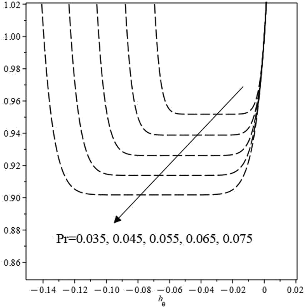
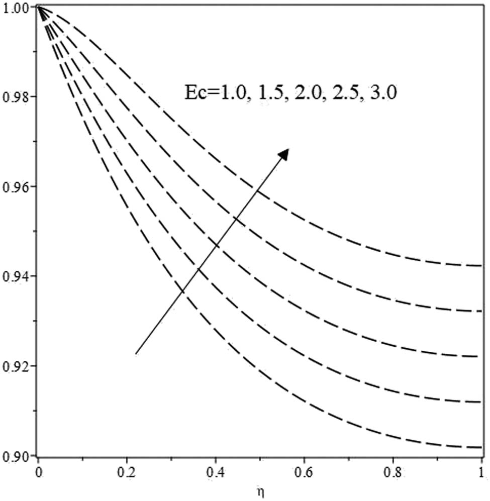
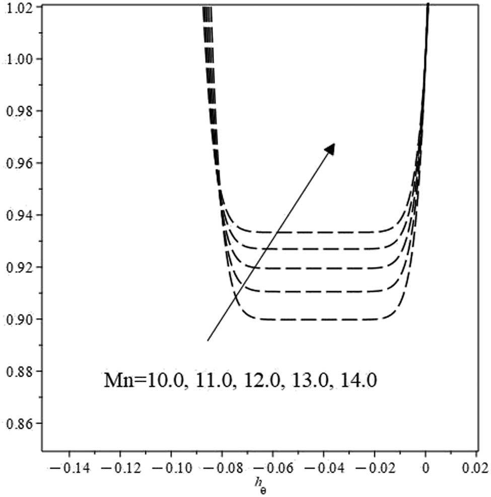
First, we draw
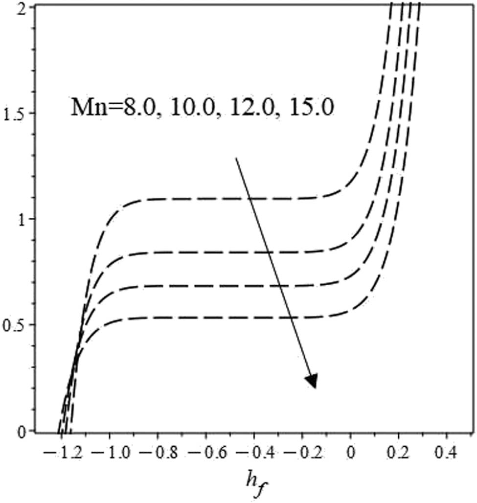
Variation in

Variation in

Variation in
Similarly, in Figures 4 and 5, same trends for the dimensionless film thickness are obtained with a variation, i.e., an increase in

Variation in

Variation in
Variation in velocity with
|
|
|
|---|---|
|
|
|
|
|
|
|
|
|
|
|
|
|
|
|
|
|
|

Variation in

Variation in


Variation in

Variation in

Variation in

Variation in

Variation in

Variation in

Variation in
4.2 Homotopy solutions for system of ODEs derived using
Z
4
The system in this case contains an arbitrary constant


Variation in

Variation in

Variation in

Variation in


Variation in
A comparison of both the cases in (4.1) and (4.2) shows that in response to an increase in the Casson parameter both the reduced systems corresponding to
5 Conclusion
We study flow and heat transfer in a Casson fluid thin film on an unsteady stretching sheet. A magnetic field is imposed on the considered flow model along with the viscous dissipation. One approach out of many that are practiced for these kinds of flow problems is the reduction of the flow model equations to their simplest possible forms. That is a transformation of the PDEs to ODEs. This is achieved with similarity transformations. The problem we are dealing with has been considered earlier, and the same procedure has been applied to it to construct corresponding velocity and temperature profiles. In this article, we derive new classes of similarity transformations using the Lie symmetry method. It provides us with more than one such transformation that enables different kinds of reductions of the flow PDEs to ODEs. The similarity transformation used here is named Lie similarity transformation. By employing it, we provide an invertible conversion of the flow PDEs to ODEs on which we apply the homotopy analysis method to construct and analyze the flow and heat transfer. The purpose of obtaining multiple classes for the similarity transformations is the optimization of the flow and heat transfer within a liquid film. Multiple similarity transformations yield different types of reductions of the flow PDEs, and hence, different kinds of flow and heat transfer patterns are revealed through analytic solutions of the obtained systems of ODEs. We presented variations in velocity and temperature profiles due to the magnetic, Casson and unsteadiness parameters, Prandtl, and Eckert numbers with the derived analytic solutions. All these dimensionless parameters and numbers are imposed in our study due to the form of similarity transformations we provided. Furthermore, the particular ranges for these parameters and numbers that are considered in this study are determined through the
To extend this study, one may construct an optimal system for the Lie symmetries of such flow equations to deduce all reducible inequivalent classes of systems of ODEs corresponding to flow PDEs. In this way, all distinct analytic solutions can be deduced which exist due to the Lie similarity procedure and HAM. As mentioned earlier with the distinct multiple solutions of a flow problem, an optimization or in other words a control on the flow and heat transfer can be attained according to the requirements of the flow problem under consideration.
Acknowledgments
The authors extend their appreciation to the Deanship of Scientific Research at King Khalid University for funding this work through a large group Research Project under grant number RGP2/47/44.
-
Funding information: Research Project under grant number RGP2/47/44 from Deanship of Scientific Research at King Khalid University.
-
Author contributions: All authors have accepted responsibility for the entire content of this manuscript and approved its submission.
-
Conflict of interest: The authors state no conflict of interest.
References
[1] Abel MS, Mahesha N, Tawade J. Heat transfer in a liquid film over an unsteady stretching surface with viscous dissipation in presence of external magnetic field. Appl Math Model. 2009;33(8):3430–41.Search in Google Scholar
[2] Abel MS, Tawade J, Nandeppanavar MM. Effect of non-uniform heat source on MHD heat transfer in a liquid film over an unsteady stretching sheet. Int J Non-Linear Mech. 2009;44(9):990–8.Search in Google Scholar
[3] Andersson HI, Aarseth JB, Dandapat BS. Heat transfer in a liquid film on an unsteady stretching surface. Int J Heat Mass Transf. 2000;43(1):69–74.Search in Google Scholar
[4] Aziz R, Hashim I, Abbasbandy S. Flow and heat transfer in a nanofluid thin film over an unsteady stretching sheet. Sains Malaysiana. 2018;47(7):1599–605.Search in Google Scholar
[5] Aziz RC, Hashim I, Alomari A. Thin film flow and heat transfer on an unsteady stretching sheet with internal heating. Meccanica. 2011;46(2):349–57.Search in Google Scholar
[6] Char MI. Heat transfer of a continuous, stretching surface with suction or blowing. J Math Anal Appl. 1988;135(2):568–80.Search in Google Scholar
[7] Chen CH. Effect of viscous dissipation on heat transfer in a non-Newtonian liquid film over an unsteady stretching sheet. J Non-Newtonian Fluid Mech. 2006;135(2–3):128–35.Search in Google Scholar
[8] Chen CH. Heat transfer in a power-law fluid film over a unsteady stretching sheet. Heat Mass Transf. 2003;39(8):791–6.Search in Google Scholar
[9] Crane LJ. Flow past a stretching plate. Zeitschrift für angewandte Mathematik und Physik. ZAMP. 1970;21(4):645–7.Search in Google Scholar
[10] Gupta P, Gupta A. Heat and mass transfer on a stretching sheet with suction or blowing. Can J Chem Eng. 1977;55(6):744–6.Search in Google Scholar
[11] Liu IC, Andersson HI. Heat transfer in a liquid film on an unsteady stretching sheet. Int J Therm Sci. 2008;47(6):766–72.Search in Google Scholar
[12] Mahmoud MA, Megahed AM. MHD flow and heat transfer in a non-Newtonian liquid film over an unsteady stretching sheet with variable fluid properties. Can J Phys. 2009;87(10):1065–71.Search in Google Scholar
[13] Megahed A. Effect of slip velocity on Casson thin film flow and heat transfer due to unsteady stretching sheet in presence of variable heat flux and viscous dissipation. Appl Math Mech. 2015;36(10):1273–84.Search in Google Scholar
[14] Ali L, Liu X, Ali B, Mujeed S, Abdal S. Finite element simulation of multi-slip effects on unsteady MHD bioconvective micropolar nanofluid flow over a sheet with solutal and thermal convective boundary conditions. Coatings. 2019;9(12):842.Search in Google Scholar
[15] Ali L, Ali B, Liu X, Iqbal T, Zulqarnain RM, Javid M. A comparative study of unsteady MHD Falkner–Skan wedge flow for non-Newtonian nanofluids considering thermal radiation and activation energy. Chin J Phys. 2022;77:1625–38.Search in Google Scholar
[16] Ali L, Ali B, Ghori MB. Melting effect on Cattaneo–Christov and thermal radiation features for aligned MHD nanofluid flow comprising microorganisms to leading edge: FEM approach. Comput Math Appl. 2022;109:260–9.Search in Google Scholar
[17] Kumar P, Poonia H, Ali L, Areekara S. The numerical simulation of nanoparticle size and thermal radiation with the magnetic field effect based on tangent hyperbolic nanofluid flow. Case Stud Therm Eng. 2022;37:102247.Search in Google Scholar
[18] Liao S. Beyond perturbation: introduction to the homotopy analysis method. New York: Chapman and Hall/CRC; 2003.Search in Google Scholar
[19] Wang C. Analytic solutions for a liquid film on an unsteady stretching surface. Heat Mass Transf. 2006;42(8):759–66.Search in Google Scholar
[20] Aziz T, Mahomed F. Applications of group theoretical methods to non-newtonian fluid flow models: survey of results. Math Probl Eng. 2017;2017:6847647.Search in Google Scholar
[21] Vijaya N, Sreelakshmi K, Sarojamma G. Effect of magnetic field on the flow and heat transfer in a Casson thin film on an unsteady stretching surface in the presence of viscous and internal heating. Open J Fluid Dyn. 2016;6(4):303–20.Search in Google Scholar
[22] Safdar M, Khan MI, Taj S, Malik MY, Shi QH. Construction of similarity transformations and analytic solutions for a liquid film on an unsteady stretching sheet using lie point symmetries. Chaos Solitons Fractals. 2021;150:111115.Search in Google Scholar
[23] Safdar M, Ijaz Khan M, Khan RA, Taj S, Abbas F, Elattar S, et al. Analytic solutions for the MHD flow and heat transfer in a thin liquid film over an unsteady stretching surface with Lie symmetry and homotopy analysis method. Waves Random Complex Media. 2022;1–19.Search in Google Scholar
[24] Taj S, Khan MI, Safdar M, Elattar S, Galal AM. Lie symmetry analysis of heat transfer in a liquid film over an unsteady stretching surface with viscous dissipation and external magnetic field. Waves Random Complex Media. 2022;1–16.Search in Google Scholar
[25] Wang F, Safdar M, Jamil B, Khan MI, Taj S, Malik MY, et al. One-dimensional optimal system of Lie sub-algebra and analytic solutions for a liquid film fluid flow. Chin J Phys. 2022;78:220–33.Search in Google Scholar
[26] Li X, Dong Z, Wang L, Niu X, Yamaguchi H, Li D, et al. A magnetic field coupling fractional step lattice Boltzmann model for the complex interfacial behavior in magnetic multiphase flows. Appl Math Model. 2023;117:219–50. 10.1016/j.apm.2022.12.025.Search in Google Scholar
[27] Liu W, Zhao C, Zhou Y, Xu X, Rakkesh RA. Modeling of Vapor-Liquid equilibrium for electrolyte solutions based on COSMO-RS interaction. J Chem. 2022;2022:9070055. 10.1155/2022/9070055.Search in Google Scholar
[28] Pang X, Zhao Y, Gao X, Wang G, Sun H, Yin J, et al. Two-step colloidal synthesis of micron-scale Bi2O2Se nanosheets and their electrostatic assembly for thin-film photodetectors with fast response. Chin Chem Lett. 2021;32(10):3099–104.Search in Google Scholar
[29] Yao J, Kong J, Kong L, Wang X, Shi W, Lu C. The phosphorescence nanocomposite thin film with rich oxygen vacancy: Towards sensitive oxygen sensor. Chin Chem Lett. 2022;33(8):3977–80.Search in Google Scholar
© 2023 the author(s), published by De Gruyter
This work is licensed under the Creative Commons Attribution 4.0 International License.
Articles in the same Issue
- Regular Articles
- Dynamic properties of the attachment oscillator arising in the nanophysics
- Parametric simulation of stagnation point flow of motile microorganism hybrid nanofluid across a circular cylinder with sinusoidal radius
- Fractal-fractional advection–diffusion–reaction equations by Ritz approximation approach
- Behaviour and onset of low-dimensional chaos with a periodically varying loss in single-mode homogeneously broadened laser
- Ammonia gas-sensing behavior of uniform nanostructured PPy film prepared by simple-straightforward in situ chemical vapor oxidation
- Analysis of the working mechanism and detection sensitivity of a flash detector
- Flat and bent branes with inner structure in two-field mimetic gravity
- Heat transfer analysis of the MHD stagnation-point flow of third-grade fluid over a porous sheet with thermal radiation effect: An algorithmic approach
- Weighted survival functional entropy and its properties
- Bioconvection effect in the Carreau nanofluid with Cattaneo–Christov heat flux using stagnation point flow in the entropy generation: Micromachines level study
- Study on the impulse mechanism of optical films formed by laser plasma shock waves
- Analysis of sweeping jet and film composite cooling using the decoupled model
- Research on the influence of trapezoidal magnetization of bonded magnetic ring on cogging torque
- Tripartite entanglement and entanglement transfer in a hybrid cavity magnomechanical system
- Compounded Bell-G class of statistical models with applications to COVID-19 and actuarial data
- Degradation of Vibrio cholerae from drinking water by the underwater capillary discharge
- Multiple Lie symmetry solutions for effects of viscous on magnetohydrodynamic flow and heat transfer in non-Newtonian thin film
- Thermal characterization of heat source (sink) on hybridized (Cu–Ag/EG) nanofluid flow via solid stretchable sheet
- Optimizing condition monitoring of ball bearings: An integrated approach using decision tree and extreme learning machine for effective decision-making
- Study on the inter-porosity transfer rate and producing degree of matrix in fractured-porous gas reservoirs
- Interstellar radiation as a Maxwell field: Improved numerical scheme and application to the spectral energy density
- Numerical study of hybridized Williamson nanofluid flow with TC4 and Nichrome over an extending surface
- Controlling the physical field using the shape function technique
- Significance of heat and mass transport in peristaltic flow of Jeffrey material subject to chemical reaction and radiation phenomenon through a tapered channel
- Complex dynamics of a sub-quadratic Lorenz-like system
- Stability control in a helicoidal spin–orbit-coupled open Bose–Bose mixture
- Research on WPD and DBSCAN-L-ISOMAP for circuit fault feature extraction
- Simulation for formation process of atomic orbitals by the finite difference time domain method based on the eight-element Dirac equation
- A modified power-law model: Properties, estimation, and applications
- Bayesian and non-Bayesian estimation of dynamic cumulative residual Tsallis entropy for moment exponential distribution under progressive censored type II
- Computational analysis and biomechanical study of Oldroyd-B fluid with homogeneous and heterogeneous reactions through a vertical non-uniform channel
- Predictability of machine learning framework in cross-section data
- Chaotic characteristics and mixing performance of pseudoplastic fluids in a stirred tank
- Isomorphic shut form valuation for quantum field theory and biological population models
- Vibration sensitivity minimization of an ultra-stable optical reference cavity based on orthogonal experimental design
- Effect of dysprosium on the radiation-shielding features of SiO2–PbO–B2O3 glasses
- Asymptotic formulations of anti-plane problems in pre-stressed compressible elastic laminates
- A study on soliton, lump solutions to a generalized (3+1)-dimensional Hirota--Satsuma--Ito equation
- Tangential electrostatic field at metal surfaces
- Bioconvective gyrotactic microorganisms in third-grade nanofluid flow over a Riga surface with stratification: An approach to entropy minimization
- Infrared spectroscopy for ageing assessment of insulating oils via dielectric loss factor and interfacial tension
- Influence of cationic surfactants on the growth of gypsum crystals
- Study on instability mechanism of KCl/PHPA drilling waste fluid
- Analytical solutions of the extended Kadomtsev–Petviashvili equation in nonlinear media
- A novel compact highly sensitive non-invasive microwave antenna sensor for blood glucose monitoring
- Inspection of Couette and pressure-driven Poiseuille entropy-optimized dissipated flow in a suction/injection horizontal channel: Analytical solutions
- Conserved vectors and solutions of the two-dimensional potential KP equation
- The reciprocal linear effect, a new optical effect of the Sagnac type
- Optimal interatomic potentials using modified method of least squares: Optimal form of interatomic potentials
- The soliton solutions for stochastic Calogero–Bogoyavlenskii Schiff equation in plasma physics/fluid mechanics
- Research on absolute ranging technology of resampling phase comparison method based on FMCW
- Analysis of Cu and Zn contents in aluminum alloys by femtosecond laser-ablation spark-induced breakdown spectroscopy
- Nonsequential double ionization channels control of CO2 molecules with counter-rotating two-color circularly polarized laser field by laser wavelength
- Fractional-order modeling: Analysis of foam drainage and Fisher's equations
- Thermo-solutal Marangoni convective Darcy-Forchheimer bio-hybrid nanofluid flow over a permeable disk with activation energy: Analysis of interfacial nanolayer thickness
- Investigation on topology-optimized compressor piston by metal additive manufacturing technique: Analytical and numeric computational modeling using finite element analysis in ANSYS
- Breast cancer segmentation using a hybrid AttendSeg architecture combined with a gravitational clustering optimization algorithm using mathematical modelling
- On the localized and periodic solutions to the time-fractional Klein-Gordan equations: Optimal additive function method and new iterative method
- 3D thin-film nanofluid flow with heat transfer on an inclined disc by using HWCM
- Numerical study of static pressure on the sonochemistry characteristics of the gas bubble under acoustic excitation
- Optimal auxiliary function method for analyzing nonlinear system of coupled Schrödinger–KdV equation with Caputo operator
- Analysis of magnetized micropolar fluid subjected to generalized heat-mass transfer theories
- Does the Mott problem extend to Geiger counters?
- Stability analysis, phase plane analysis, and isolated soliton solution to the LGH equation in mathematical physics
- Effects of Joule heating and reaction mechanisms on couple stress fluid flow with peristalsis in the presence of a porous material through an inclined channel
- Bayesian and E-Bayesian estimation based on constant-stress partially accelerated life testing for inverted Topp–Leone distribution
- Dynamical and physical characteristics of soliton solutions to the (2+1)-dimensional Konopelchenko–Dubrovsky system
- Study of fractional variable order COVID-19 environmental transformation model
- Sisko nanofluid flow through exponential stretching sheet with swimming of motile gyrotactic microorganisms: An application to nanoengineering
- Influence of the regularization scheme in the QCD phase diagram in the PNJL model
- Fixed-point theory and numerical analysis of an epidemic model with fractional calculus: Exploring dynamical behavior
- Computational analysis of reconstructing current and sag of three-phase overhead line based on the TMR sensor array
- Investigation of tripled sine-Gordon equation: Localized modes in multi-stacked long Josephson junctions
- High-sensitivity on-chip temperature sensor based on cascaded microring resonators
- Pathological study on uncertain numbers and proposed solutions for discrete fuzzy fractional order calculus
- Bifurcation, chaotic behavior, and traveling wave solution of stochastic coupled Konno–Oono equation with multiplicative noise in the Stratonovich sense
- Thermal radiation and heat generation on three-dimensional Casson fluid motion via porous stretching surface with variable thermal conductivity
- Numerical simulation and analysis of Airy's-type equation
- A homotopy perturbation method with Elzaki transformation for solving the fractional Biswas–Milovic model
- Heat transfer performance of magnetohydrodynamic multiphase nanofluid flow of Cu–Al2O3/H2O over a stretching cylinder
- ΛCDM and the principle of equivalence
- Axisymmetric stagnation-point flow of non-Newtonian nanomaterial and heat transport over a lubricated surface: Hybrid homotopy analysis method simulations
- HAM simulation for bioconvective magnetohydrodynamic flow of Walters-B fluid containing nanoparticles and microorganisms past a stretching sheet with velocity slip and convective conditions
- Coupled heat and mass transfer mathematical study for lubricated non-Newtonian nanomaterial conveying oblique stagnation point flow: A comparison of viscous and viscoelastic nanofluid model
- Power Topp–Leone exponential negative family of distributions with numerical illustrations to engineering and biological data
- Extracting solitary solutions of the nonlinear Kaup–Kupershmidt (KK) equation by analytical method
- A case study on the environmental and economic impact of photovoltaic systems in wastewater treatment plants
- Application of IoT network for marine wildlife surveillance
- Non-similar modeling and numerical simulations of microploar hybrid nanofluid adjacent to isothermal sphere
- Joint optimization of two-dimensional warranty period and maintenance strategy considering availability and cost constraints
- Numerical investigation of the flow characteristics involving dissipation and slip effects in a convectively nanofluid within a porous medium
- Spectral uncertainty analysis of grassland and its camouflage materials based on land-based hyperspectral images
- Application of low-altitude wind shear recognition algorithm and laser wind radar in aviation meteorological services
- Investigation of different structures of screw extruders on the flow in direct ink writing SiC slurry based on LBM
- Harmonic current suppression method of virtual DC motor based on fuzzy sliding mode
- Micropolar flow and heat transfer within a permeable channel using the successive linearization method
- Different lump k-soliton solutions to (2+1)-dimensional KdV system using Hirota binary Bell polynomials
- Investigation of nanomaterials in flow of non-Newtonian liquid toward a stretchable surface
- Weak beat frequency extraction method for photon Doppler signal with low signal-to-noise ratio
- Electrokinetic energy conversion of nanofluids in porous microtubes with Green’s function
- Examining the role of activation energy and convective boundary conditions in nanofluid behavior of Couette-Poiseuille flow
- Review Article
- Effects of stretching on phase transformation of PVDF and its copolymers: A review
- Special Issue on Transport phenomena and thermal analysis in micro/nano-scale structure surfaces - Part IV
- Prediction and monitoring model for farmland environmental system using soil sensor and neural network algorithm
- Special Issue on Advanced Topics on the Modelling and Assessment of Complicated Physical Phenomena - Part III
- Some standard and nonstandard finite difference schemes for a reaction–diffusion–chemotaxis model
- Special Issue on Advanced Energy Materials - Part II
- Rapid productivity prediction method for frac hits affected wells based on gas reservoir numerical simulation and probability method
- Special Issue on Novel Numerical and Analytical Techniques for Fractional Nonlinear Schrodinger Type - Part III
- Adomian decomposition method for solution of fourteenth order boundary value problems
- New soliton solutions of modified (3+1)-D Wazwaz–Benjamin–Bona–Mahony and (2+1)-D cubic Klein–Gordon equations using first integral method
- On traveling wave solutions to Manakov model with variable coefficients
- Rational approximation for solving Fredholm integro-differential equations by new algorithm
- Special Issue on Predicting pattern alterations in nature - Part I
- Modeling the monkeypox infection using the Mittag–Leffler kernel
- Spectral analysis of variable-order multi-terms fractional differential equations
- Special Issue on Nanomaterial utilization and structural optimization - Part I
- Heat treatment and tensile test of 3D-printed parts manufactured at different build orientations