Analysis of sweeping jet and film composite cooling using the decoupled model

Xiangcan Kong; Yanfeng Zhang; Guoqing Li; Xingen Lu; Jun Zeng; Junqiang Zhu; Jinliang Xu

doi:10.1515/phys-2022-0238

Article Open Access

Analysis of sweeping jet and film composite cooling using the decoupled model

Xiangcan Kong , Yanfeng Zhang , Guoqing Li , Xingen Lu , Jun Zeng , Junqiang Zhu and Jinliang Xu

Published/Copyright: March 25, 2023

Published by

Become an author with De Gruyter Brill

Submit Manuscript Author Information Explore this Subject

From the journal Open Physics Volume 21 Issue 1

Abstract

The heat transfer process of the sweeping jet and film composite cooling (SJF) structure of the turbine blade leading edge is complex. The current work divides the overall cooling effectiveness of the SJF into the impingement heat transfer effectiveness, the convection heat transfer effectiveness inside the film holes, and the external film cooling effectiveness by the decoupled method. Various cooling effectiveness proportions and trends are compared when the blowing ratios are 1.05, 2.07, and 4.11. There is an average ratio of 64.33% for impingement heat transfer effectiveness and 38.02% for convection heat transfer effectiveness. The ratio of external film cooling effectiveness gradually changes from positive to negative with the increase of the blowing ratio. Therefore, the proportion of external film cooling effectiveness and impingement heat transfer effectiveness should be considered when applying SJF. The convection heat transfer effectiveness cannot be ignored, especially when the design scheme of the shower head is used.

Keywords: conjugate heat transfer; decoupled model; composite cooling; sweeping jet cooling

Nomenclature

D: hydraulic diameter of the exit throat, mm
d _f: diameter of the film hole, mm
D _LE,out: outer diameter of the leading edge, mm
D _LE,in: inner diameter of the leading edge, mm
H _c: height of the coolant channel, mm
H _f: pitch of film holes, mm
H _i: height of the solid domain of the fluidic oscillator, mm
L _i: length of the solid domain of the fluidic oscillator, mm
M: blowing ratio
Nu: Nusselt number
T: temperature, K
t _imp: thickness of the impingement plate, mm
t _LE: thickness of the leading edge, mm
u _τ: shear velocity, m/s
W _i: weight of the solid domain of the fluidic oscillator, mm
X: axial coordinate value, mm
Y: mainstream coordinate value, mm
y: thickness of the first grid, mm
y ⁺: non-dimensional distance (= yu _τ/υ)
Z: spanwise coordinate value, mm

Greek symbols

η: overall cooling effectiveness
η _ad: adiabatic cooling effectiveness
η _ex: external cooling effectiveness
η _fh: convection cooling effectiveness in film holes
η _imp: internal impingement cooling effectiveness
η _in: internal cooling effectiveness
ρ: density, kg/m³
υ: kinematic viscosity, m²/s
Φ: phase angle, °

Acronyms

CHT: conjugate heat transfer model
DEM: decoupled model
F: film hole
POD: proper orthogonal decomposition
SJF: sweeping jet and film composite cooling
NJF: normal jet and film composite cooling
OCE: overall cooling effectiveness

1 Introduction

There is a need to consider turbine cooling structures in turbine design because turbine cooling structures can make a turbine work beyond the melting point of the materials used in blades. The research on new cooling fluids, such as nanofluid [1,2], is particularly important; besides, a variety of turbine cooling structures have been studied extensively through experimental work and numerical simulations in order to better understand how they work. As far as the numerical simulation is concerned, conjugate heat transfer can produce a more accurate prediction of the cooling effectiveness than adiabatic calculation [3,4]. The conjugate heat transfer method considers the heat conduction process of the solid, and the thermal conductivity of the turbine blade material will also affect the cooling effectiveness. At present, the blade material is constantly evolving; thus, the derivation of the thermal conductivity equation with variable thermal conductivity and time-fractional order in special materials [5,6] has also become an important research direction.

As a result of the impingement and the film composite cooling structure that is used to cool the leading edge of the turbine blades, it is extremely difficult to determine the optimal value of the overall cooling effectiveness (OCE). If the impingement heat transfer effectiveness is high, there will be a relatively low-temperature difference between the coolant and the mainstream formed when the film is formed, decreasing the film cooling effectiveness. To better understand the proportion of the impingement heat transfer effectiveness (η _imp), convection heat transfer effectiveness inside the film holes (η _fh), and external film cooling effectiveness (η _ex) in the OCE, Zhou et al. [7] developed a decoupled model to take into account these variables. The decoupled model is explained in detail in Section 2.6. As shown by Zhou et al. [7], η _imp accounts for about 70% of the OCE of the traditional impingement and film composite cooling structure, η _fh accounts for about 30%, η _ex represents the smallest proportion of the OCE, and it can have a negative effect on a large blowing ratio. A further problem with the decoupled model is that η _ex is not the same as the adiabatic film cooling effectiveness (η _ad) in the adiabatic model, as it is not governed by the same assumptions. The decoupled model considers the solid heat conduction as part of η _ex, whereas in the adiabatic model, η _ad does not consider the heat conduction of the solid at all.

Turbine blade leading edges are usually cooled with an impingement and the film composite structure. Film holes are usually arranged densely in a composite cooling structure, which can be compared to a showerhead. However, the impingement nozzles can take a variety of forms, such as the traditional cylindrical normal jet nozzle [8], cylindrical tangential jet nozzle [9], slot tangential jet nozzle [10], convergent staggered jet nozzle [11], and sweeping jet nozzle [12]. Significantly, the sweeping jet nozzle, also known as a fluidic oscillator, was proposed by the Bowles Fluidic Corporation in 1979 [13]. It is widely used for flow control [14], noise reduction [15], and resistance reduction [16], and due to its sweeping characteristics, it has been used as film holes [17] and impingement nozzles [18] on turbine blades in recent years. There has been experimental evidence that when the dimensionless impinging distance is greater than 4, the same amount of coolant flow rate can achieve a greater η _imp for the sweeping jet impingement nozzle [19]. There is also a considerable improvement in the OCE of the sweeping jet and film composite cooling (SJF) structure over that of the conventional normal jet and film composite cooling structure (NJF) when applied to the flat plate [20] and curved surface [12] with film holes. Moreover, the OCE of the tangential jet and film composite cooling structure is equivalent to that of the NJF [9,21]. Consequently, if the turbine blade allows a large inlet total pressure to flow into the cooling structure, the OCE of the SJF will be greater than that of other composite cooling structures.

However, the configuration of film holes and impingement jet nozzle of SJF proposed in the study of Kong et al. [12] only represents the conventional scheme and cannot obtain the optimal OCE; the current work is to explore the proportion of η _imp, η _fh, and η _ex in the OCE for the SJF, which can provide a reference for SJF in the global optimization of the geometry such as the location and diameter of the film holes. Another purpose of the current work is to show the universality of the decoupling method, which can analyze the various cooling effectiveness of the SJF, a complex structure on a curved surface. Therefore, the decoupling method can still be applied to the cooling effectiveness analysis of SJF on the real blade leading edge under the conditions similar to the semi-cylindrical leading-edge model. The SJF in the study of Kong et al. [12] is selected for specific decoupling analysis, and the working conditions with blowing ratios of 1.05, 2.07, and 4.11 are selected for simulation calculation; the solid domain is removed to obtain η _ad in the composite cooling structure to prove the negative effect of η _ex in the decoupled model.

2 Geometry and decoupled model

2.1 Geometry

Based on the study of Kong et al. [12], the SJF is chosen as the focus of a research project in this study as illustrated in Figure 1. It is designed to simulate the blade's leading-edge by using a leading-edge model and a fluidic oscillator, which are both static models. This leading-edge model has a sweeping jet nozzle (fluidic oscillator, shown in Figure 2) and a total of 15 film holes that are arranged. This model is a semi-cylinder that is extended on both sides and has a hollowed-out impingement plate to close it. The impinging distance is defined as the gap from the fluidic oscillator throat to the middle row of film holes (4D in this article). This semi-cylinder is cooled by three film hole rows that are placed on its outer surface. There are five holes in each row that are tilted 25° to the outer surface of the semi-cylinder, each hole holding three angles of 0 and 30° to the axial direction, and the geometric details are described in Table 1. The sweeping jet nozzle is a fluidic oscillator device, which is modified following Bowles Fluidic Corporation [13]. There is a thickness D to the fluidic oscillator. The three-dimensional physical model of the current work is consistent with that of Kong et al. [12], as shown in Figure 3. The coolant flows along the outer surface of the semi-cylinder through the film holes after it has been injected into the fluidic oscillator, preventing the frontal scouring with the mainstream.

Figure 1

Details of the dimensions and the arrangements.

Figure 2

Various parts and geometric dimensions of the fluidic oscillator [13].

Table 1

Details of the dimensions

Dimension	Value (mm)	Dimension	Value (mm)
D	1.0	H _i	12.1
d _f	0.3	L _i	9.0
D _LE,in	7.0	W _i	3.0
D _LE,out	9.0	H _c	19.0
t _LE	1.0	H _f	1.5
t _imp	1.0

Figure 3

The leading-edge model [12].

2.2 Computation model procedure

Commercial software CFX 19.0 is being used in the current project, as well as the URANS and SST k–ω turbulence model. Since the compressible coolant is compressed and expanded in the fluidic oscillator, the compressibility of the fluid is considered. Therefore, the URANS equations [22] are as follows:

(1) ∂ ρ ∂ t + ∂ ∂ x j ( ρ U j ) = 0 ,

(2) ∂ ∂ t ( ρ U j ) + U i ∂ ∂ x i ( ρ U j ) = − ∂ P ∂ x j + ∂ ∂ x i μ ∂ U j ∂ x i ¯ − ρ U i ' U j ' ,

(3) ∂ ∂ t ( ρ c P T ) + U i ∂ ∂ x i ( ρ c P T ) = ∂ ∂ x i λ ∂ T ∂ x i ¯ − ρ c P U i ' T ' .

Assume that the solid domain is solved in the conjugate heat transfer model; then the following energy equation applies:

(4) ∂ ρ s c Ps T ∂ t = ∇ ⋅ ( λ s ⋅ ∇ T s ) ,

where U, U′, ρ, P, c _P, T, T′, and λ are the velocity vector (m/s), velocity pulsation (m/s), density (kg/m³), pressure (Pa), the specific heat (J/(kg K)), temperature (K), temperature pulsation (K), and thermal conductivity coefficient (W/(m K)), respectively. Subscript s represents the variable in the solid domain.

The reason for choosing the SST k–ω turbulence model is that it can solve the flow field with a strong pressure gradient and accurately capture the phenomenon of flow separation [23]. The SST k–ω turbulence model is a two-equation model, which is composed of the k–ω model and can solve the flow near the wall, and the k–ε model, which can solve the free-stream flow outside the wall, given by

(5) ∂ ( ρ k ) ∂ t + ∂ ( ρ U i k ) ∂ x i = P k − β ∗ ρ k ω + ∂ ∂ x i ( μ + σ k μ t ) ∂ k ∂ x i ,

(6) ∂ ( ρ ω ) ∂ t + ∂ ( ρ U i ω ) ∂ x i = α ρ S 2 − β ρ ω 2 + ∂ ∂ x i ( μ + σ ω μ t ) ∂ ω ∂ x i + 2 ( 1 − F 1 ) ρ σ ω 2 1 ω ∂ k ∂ x i ∂ ω ∂ x i .

The turbulent eddy viscosity is given by

(7) ν t = a 1 k max ( a 1 ω , S F 2 ) .

In addition, some important terms in Eqs. (5)–(7) are given by

(8) P k = min τ i j ∂ U i ∂ x j , 10 ⋅ β ∗ ρ k ω ,

(9) τ i j = 2 ν t S i j − 2 3 δ i j k ,

(10) S = 2 S i j S i j , S i j = 1 2 ∂ U i ∂ x j + ∂ U j ∂ x i ,

(11) F 1 = tanh min max k β ∗ ω y , 500 ν y 2 ω , 4 ρ σ ω 2 k CD k ω y 2 4 ,

where F ₁ = 0 is the blending coefficient, away from the surface (k–ε model) and increases to 1 inside the boundary layer (k–ω model). y is the distance to the nearest wall.

(12) CD kω = max 2 ρ σ ω 2 1 ω ∂ k ∂ x i ∂ ω ∂ x i , 10 − 10 .

F ₂ is the second blending coefficient and is given by

(13) F 2 = tanh max 2 k β ∗ ω y , 500 ν y 2 ω 2 .

All constants are computed by a blend from the corresponding constants of the k–ε and k–ω models via α = α ₁ F + α ₂(1−F),…. The constants for this model are α ₁ = 5/9, α ₂ = 0.44, β ₁ = 3/40, β ₂ = 0.0828, β* = 0.09, σ _k1 = 0.85, σ _k2 = 1, σ _ω1 = 0.5, and σ _ω2 = 0.856.

2.3 Boundary conditions

Both the coolant and the mainstream are assumed to be air-ideal gases. The coolant mass flow rate is set as a function of the blowing ratio, while the total temperatures of the mainstream and coolant are set to 480 and 300 K, respectively, resulting in the temperature ratio being 0.625. In each of the different cases, the mainstream and coolant turbulent intensity is 1%; Table 2 lists the important boundary conditions that have been applied. In the calculation domain, there are translational periods on the upper and lower sides. Interface boundaries are set on the surfaces which are in contact with fluids and solids, while non-slip adiabatic walls are set on the other surfaces. It is convergent when all three, mass, energy, and momentum conservation equations, have root-mean-square residences below 1 × 10⁻⁶.

Table 2

Boundary conditions

Mainstream temperature, T _m (K)	480
Mainstream inlet velocity, V _in,m (m/s)	40, 32, 26.7
Outlet static pressure, P _out (Pa)	101,325
Coolant inlet temperature, T _c (K)	300
Temperature ratio, T _c/T _m	0.625
Blowing ratios, ρ _c V _c/ρ _m V _m	1.05, 2.07, 4.11

2.4 Grid and turbulence model

In order to generate the hexahedral grid for the sweeping jet, the Workbench commercial software meshing module was used, while in order to obtain the hexahedral grid for the other fluid domain and solid domain, ICEM CFD was employed. Figure 4 indicates the grid near the sweeping jet and film holes. An O-type subdivision is utilized for the blocks of film holes and a Y-type subdivision is used for discretizing the blocks of the impingement chamber on both ends. The low-Reynolds number k–ω turbulence model would require at least y ⁺ < 1; therefore, a careful adjustment is made to the height of the first grid in the fluid domain so that the y ⁺ value remains less than 1 in all different cases.

Figure 4

Blocks and grid of the physic model. (a) Mesh of the fluidic oscillator. (b) Mesh of the film holes. (c) The edges of blocks of the mainstream chamber. (d) The edges of blocks of the impingement chamber.

Kong et al. [12] have proved that the SST k–ω turbulence model can more accurately predict the cooling effectiveness of the SJF. The current work still uses this turbulence model to calculate the decoupled model, conjugate heat transfer model, and adiabatic model. In addition, the fluid domain grids of the decoupled model, conjugate heat transfer model, and adiabatic model also adopt the first layer grid height and grid number (about 10.40 million) of Kong et al. [12].

2.5 Definitions of parameters

This study investigates the heat transfer characteristics of SJF by defining a few parameters.

Coolant mass flow to the mainstream is characterized by the blowing ratio, which is calculated as follows:
(14) M = m c A c ρ m V m = ρ c V c ρ m V m ,
where ρ, V, and m are the density (kg/m³), velocity (m/s), and mass flow (kg/s), respectively. A _c is the area of the coolant inlet in the SJF structure.
The Nusselt number is employed to investigate the non-dimensional heat transfer coefficient of the impinging surface and is defined as follows:
(15) Nu = q w D ( T w − T in , c ) λ ,
where q _w represents the wall heat flux, λ represents the fluid thermal conductivity, and T _w represents the impinging surface temperature.
The SJF cooling performance is measured using the OCE, which is defined as follows:
(16) η = T in , m − T ow T in , m − T in , c ,
where T _ow and T _in,m are the outer wall and mainstream temperature, respectively (K).
Because the sweeping jet is a simple harmonic motion, the time-averaged value of a variable can be obtained by averaging it in a sweeping period:

(17) S − = 1 T ∫ 0 T S d t ,

where S stands for the Nu number, OCE or velocity, etc., and T is the time required to complete a sweeping period.

2.6 Decoupled model

The decoupling method is used to obtain η _imp, η _fh, and η _ex and the proportion of these cooling effectiveness in the OCE. This section focuses on the principle and implementation method of the decoupled model from the study of Zhou et al. [7]. Figure 5 shows the NJF on the flat plate: the conjugate heat transfer model is divided into the “mainstream model” and “ideal internal cooling model” at the orifices, the interface on the mainstream side is set as “wall,” the interface on the film hole side is set as “outlet,” and the solid domain and fluid domain are still connected through an “interface” for heat exchange. In the present work, there are 15 film holes and 15 interfaces are introduced. Although the coolant still flows out of the film hole outlet, it will not enter the mainstream model, which is equivalent to no film near the film holes. At this time, the cooling effectiveness obtained from the outer surface temperature of the “ideal internal cooling model” is “equivalent internal cooling effectiveness” (η _in); then η _imp and η _fh are calculated according to the “heat release rate” ratio of the inner wall surface of the impinging surface to the film holes and η _ex is obtained by η − η _in. However, η _ex is different from η _ad. Decoupled models continue to exchange heat between the solid domain and mainstream, while adiabatic models use the solid domain’s outer surface as an adiabatic wall. Therefore, η _ad can only represent the influence of the film on the cooling effectiveness of the adiabatic wall.

Figure 5

Principles of the decoupled model [7].

A very similar cooling effectiveness has been obtained by combining the boundary conditions corresponding to the conjugate heat transfer model with the decoupled model (as shown in Figure 6) to eliminate the differences between the internal flow structure of the decoupled model and the conjugate heat transfer model. As with the conjugate heat transfer model, the adiabatic model has consistent inlet and outlet boundary conditions, but the decoupled model has different outlet boundary conditions. Therefore, the decoupled model needs to adopt different boundary conditions from the conjugate heat transfer model to make the flow field structures of the two agree with each other. In the study of Zhou et al. [7], the decoupled model adopts the total pressure boundary conditions at the inlet and mass flow rate boundary conditions at the outlet. Calculations of the conjugate heat transfer model are used to determine the boundary under each working condition in the decoupled model, and the rationality of this method has been verified. In the present work, Tables 3–5 show how the mass flow rate at the orifices is different at each time due to the sweeping behavior of the jet, but the difference between the transient value and the time-averaged value is small. Therefore, the time-averaged mass flow rate is finally selected as the outlet boundary conditions of the decoupled model.

Figure 6

(a) The conjugate heat transfer model and (b) the decoupled model [7].

Table 3

Time-averaged and time-accurate mass flow rate at the outlet of each film hole for M = 1.05 (unit: mg/s)

	F1	F2	F3	F4	F5	F6	F7	F8	F9	F10	F11	F12	F13	F14	F15
Time-averaged	9.4	9.7	10.0	10.2	9.6	8.4	7.2	14.6	12.4	10.1	9.4	9.6	9.9	10.1	9.7
Φ = 0°	9.7	9.9	9.1	9.6	9.3	7.8	7.3	14.2	12.0	9.6	9.2	9.7	9.6	9.7	9.4
Φ = 60°	8.7	9.5	9.0	10.6	9.5	8.2	7.2	13.6	11.8	9.4	9.3	9.6	9.2	9.1	9.2
Φ = 120°	8.6	9.3	9.5	9.9	9.6	8.4	7.1	14.6	12.2	9.9	9.3	9.6	9.7	9.5	9.5
Φ = 180°	9.2	9.8	9.8	9.1	9.4	8.1	7.0	14.0	12.7	10.0	10.3	9.2	10.0	10.0	9.8

Table 4

Time-averaged and time-accurate mass flow rate at the outlet of each film hole for M = 2.07 (unit: mg/s)

	F1	F2	F3	F4	F5	F6	F7	F8	F9	F10	F11	F12	F13	F14	F15
Time-averaged	17.9	17.3	19.3	20.3	19.0	17.1	16.5	18.9	20.2	19.2	17.7	17.3	18.5	18.8	18.3
Φ = 0°	18.1	15.4	18.3	17.3	17.9	15.4	16.6	18.3	19.5	18.5	16.7	17.7	17.7	18.0	18.0
Φ = 60°	15.8	15.9	17.5	21.1	18.7	16.2	16.6	17.5	18.6	18.1	16.9	17.3	17.3	16.5	17.5
Φ = 120°	15.7	15.5	18.6	19.1	18.7	17.0	16.2	18.9	19.5	18.5	17.4	17.7	17.8	17.7	18.0
Φ = 180°	16.8	17.8	17.9	18.6	18.5	15.1	16.2	17.9	19.5	19.0	17.6	15.0	18.3	18.7	18.2

Table 5

Time-averaged and time-accurate mass flow rate at the outlet of each film hole for M = 4.11 (unit: mg/s)

	F1	F2	F3	F4	F5	F6	F7	F8	F9	F10	F11	F12	F13	F14	F15
Time-averaged	34.5	34.6	37.8	39.7	37.8	34.0	33.1	37.2	40.6	38.7	33.7	34.9	37.7	38.6	37.5
Φ = 0°	35.8	34.7	34.2	36.8	36.1	33.9	31.4	35.7	41.3	37.8	32.8	34.8	36.2	36.9	36.9
Φ = 60°	32.0	31.4	37.2	40.2	37.2	33.8	34.2	36.3	37.6	37.7	34.3	34.6	35.8	35.6	36.0
Φ = 120°	31.7	31.6	36.9	39.7	38.5	34.3	34.3	39.5	38.5	37.0	35.1	35.8	36.6	36.1	35.8
Φ = 180°	33.8	35.0	36.3	36.7	37.0	33.0	31.1	38.1	41.3	38.7	35.1	35.6	35.6	36.8	35.3

3 Results

3.1 Rationality of the decoupled model

For testing the effectiveness and ensuring the accuracy of the decoupling method in the present study, the working conditions of M = 2.07 will be used. In both the conjugate heat transfer model and the decoupled model, the flow structure and Nu number distribution are evaluated indexes, as shown in Figure 7(a) and (b). The decoupled model clearly exhibits the same internal flow structures and Nu number distributions as the conjugate heat transfer model. On the other hand, since the mainstream and the film are no longer mixed with each other and the external flow structure is symmetrical along the line X/D = 0, the decoupled model can perfectly eliminate the external cooling effectiveness. Therefore, the decoupling method can accurately estimate the specific values of η _imp, η _fh, and η _ex in the present work.

Figure 7

Comparison between the decoupled model and conjugate heat transfer model at M = 2.07 for the (a) flow structure and (b) internal impingement cooling effectiveness.

To better understand the physical mechanism of the complex flow inside the impingement chamber and further prove the rationality of the decoupled model, the proper orthogonal decomposition (POD) technique is used to separate and extract the coherent structures of different scales in the impingement chamber. Based on the unsteady results of the CHT scheme and DEM scheme at M = 2.07, the time interval is Δt = 0.00012 s and a total of 50 moments of data were extracted for POD analysis. Figure 8 shows the distribution of eigenvalues of the first 40 POD modes of the CHT scheme, where N is the mode number and λ is the eigenvalues, with the eigenvalues of POD being the energy of the corresponding POD modes. It can be seen from Figure 8 that the energy of the first four modes accounts for 46.2% of the total energy, and the first 20 modes account for 82.4% of the total energy (the calculation method is shown in the study of Wang et al. [24]). Therefore, the POD method reduces the order of the high-dimensional unsteady flow effectively, and the first four modes can represent the main flow characteristics.

Figure 8

The eigenvalues of POD modes for the CHT scheme.

Figure 9 depicts the contours of the local Nu number on the impinging surface of the first four POD modes for the CHT scheme and DEM scheme, and the data of each mode are normalized to facilitate comparison. The value of the Nu number in each mode is a relative value, with a large value indicating a large amplitude of vibration. It can be seen from Figure 9 that the position of the high Nu number region is different under various modes, indicating that the unsteady flow in the impingement chamber is complex and there are many vortex structures. The first mode structure mainly appears on both sides of X/D = 0; therefore, the main unsteady structure in the impingement chamber is the vortex cluster on both sides of X/D = 0, especially at Z/D = 0. The second and third mode structures focus on the right side and left side of X/D = 0, respectively. This area is the location where the jet core directly impings the impinging surface. There is a phase angle (Φ) difference between the second mode and the third mode, and the jet core shifts from the right side of X/D = 0 to the left side over time. The vibration amplitude of the fourth mode is small, which indicates that it is caused by more broken small-scale vortices. In addition, the difference between the DEM scheme and CHT scheme is small, which further indicates that the decoupled model is reasonable in SJF.

Figure 9

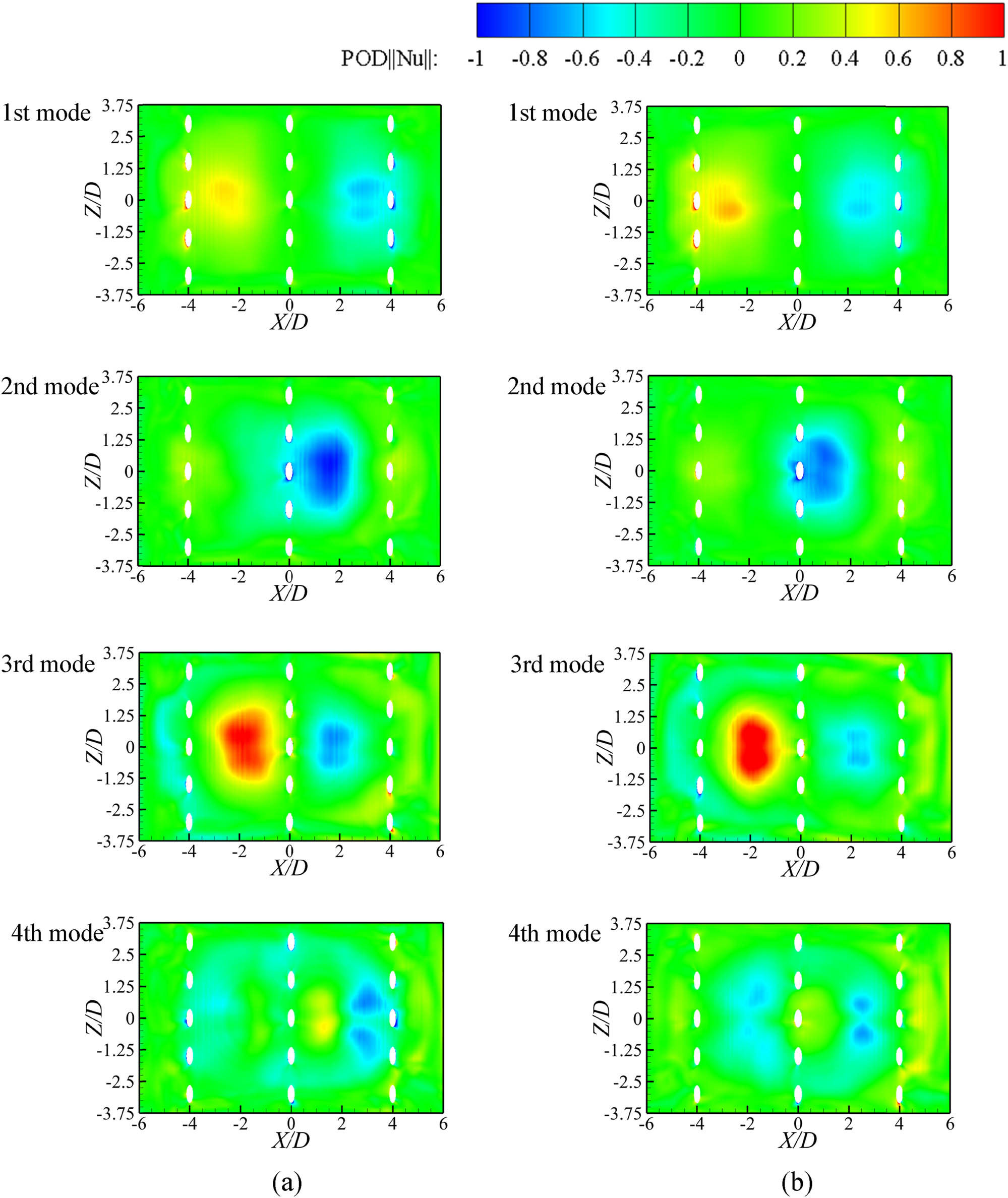
Contours of the local Nu number on the impinging surface of the first four POD modes for the (a) CHT scheme and (b) DEM scheme.

3.2 Comparative analysis of time-accurate and time-averaged contours

It is important to distinguish between the similarities and differences between the time-accurate and time-averaged data for the jet since it sweeps periodically with time. Figure 10 shows the time-accurate and time-averaged contours of the Nu number, temperature, and OCE with M = 2.07, for the conjugate heat transfer model. The peak value of the Nu number varies with time, as shown in Figure 10, while the temperature on the impinging surface hardly changes over time. When the fluid thermal conductivity is constant, according to the definition, the Nu number depends heavily on the wall heat flux. Thus, it is evident that the Nu number contour changes with time on impinging surfaces, and there is a large difference between the time-accurate contour and the time-averaged contour. However, the temperature is almost constant because it takes a short time to complete each sweep period (about 0.000515–0.000946 s in this article); keeping the jet core stationary for long periods of time is impossible and it is impossible to form an obvious temperature difference on the impinging surface. Consequently, time-accurate and time-averaged temperature contours are virtually identical. Moreover, the temperature remains almost constant, explaining why the OCE changes little with time. At the same time, the external coolant film pulsation can only cause a small temperature difference, resulting in the solid domain still exhibiting relatively constant thermal conductivity over time.

Figure 10

Time-accurate and time-averaged results of the Nu number, temperature, and OCE at M = 2.07.

Since the impinging surface temperature and the OCE of the outer surface in the SJF do not change with time, and the difference between the time-accurate distribution and the time-averaged distribution is extremely small, it is reasonable to select the time-averaged data when analyzing the proportion of each cooling effectiveness in the OCE.

3.3 Various kinds of cooling effectiveness and their proportions to OCE

Figure 11 shows the variation trend of area-averaged OCE, internal cooling effectiveness, and adiabatic cooling effectiveness with the blowing ratio. As there are only three blowing ratios in the present work, some subtle trends are not shown. For example, the adiabatic film cooling effectiveness does not increase first and then decrease with the increase of the blowing ratio but has been in a downward trend. Nevertheless, it can still be inferred from Figure 11 that the adiabatic film cooling effectiveness deteriorates the OCE under a high blowing ratio. It is because the OCE and internal cooling effectiveness increase with the increase of the blowing ratio, but when the blowing ratio increases to about 1.6, the value of internal cooling effectiveness exceeds the OCE.

Figure 11

The area-averaged OCE, internal cooling effectiveness, and adiabatic cooling effectiveness at different blowing ratios.

Figure 12 shows the specific values of η _imp, η _fh, η _ex, and OCE (η) at three blowing ratios. η _imp accounts for an average of 64.33% of the OCE in the whole blowing ratio range. η _fh becomes larger when the blowing ratio increases and its proportion in the OCE is considerable (an average of 38.02%). η _fh cannot be ignored in the turbine thermal design, especially in the showerhead leading edge of the actual blade. η _ex is positive when M = 1.05, but from its change trend, the contribution of η _ex to the OCE becomes smaller and negative. The negative effect of η _ex makes the OCE slow down with the increase of the blowing ratio, which means that the mixing of the coolant and mainstream is more intense, resulting in greater mixing loss. Therefore, in the thermal design of the turbine, the shape and installation angle of film holes are emphatically considered to reduce the negative effect of η _ex and obtain higher OCE values.

Figure 12

The values of η _imp, η _fh, η _ex, and OCE (η).

4 Conclusion

The decoupled model is used to explore the proportion of each cooling effectiveness in the OCE at different blowing ratios. The conjugate heat transfer model is also calculated as a reference for verification and to provide data such as boundary conditions in the decoupled model. The calculation results of the adiabatic model are used to prove the changing trend of the external film cooling effectiveness in the decoupled model. The results show that the decoupled model adopted in this manuscript is universal. Both the normal jet and film composite cooling structure on the plate in the study of Zhou et al. [7] and the SJF structure on the curved surface in this manuscript have obtained relatively consistent results; therefore, it can be inferred that the decoupled model can be applied to the study of the complicated actual turbine blade leading edge. It is also proposed that the research results of the current study can provide a reference and a technical path for the optimization of geometry parameters such as the number and position of film holes in the future to achieve the optimal OCE of SJF. The specific results are as follows.

The decoupled model and conjugate heat transfer model produce similar results, proving that the decoupled model can be applied to the SJF on a curved surface.
As a periodic impinging nozzle, the time-accurate temperature on the inner and outer surfaces of the leading-edge model is unchanged. So it is reasonable to analyze the proportion of η _imp, η _fh, and η _ex in the OCE by using the time-averaged results.
There is an average ratio of 64.33% for η _imp in the three blowing ratios of 1.05, 2.07, and 4.11, and 38.02% for η _fh. The ratio of η _ex gradually changes from positive to negative with the increase of the blowing ratio.
In the future, the results of the current study can be used to guide the global optimization of geometry parameters such as the number and diameter of film holes or the number of sweep impinging nozzles to change the proportion of each cooling effectiveness and achieve optimal OCE of SJF in actual blade applications.

Funding information: This work was supported by the National Science and Technology Major Project (J2019-II-0002-0022, J2019-II-0021-0042), National Natural Science Foundation of China (No. 51836008, No. 51976214), and Science Center for Gas Turbine Project (P2022-B-II-006-001).
Author contributions: All authors have accepted responsibility for the entire content of this manuscript and approved its submission.
Conflict of interest: The authors state no conflict of interest.

References

[1] Gul T, Altaf Khan M, Khan A, Shuaib M. Fractional-order three-dimensional thin-film nanofluid flow on an inclined rotating disk. Eur Phys J Plus. 2018;133(12):500.10.1140/epjp/i2018-12315-4Search in Google Scholar

[2] Gul T, Noman W, Sohail M, Khan MA. Impact of the Marangoni and thermal radiation convection on the graphene-oxide-water-based and ethylene-glycol-based nanofluids. Adv Mech Eng. 2019;11(6):1–9.10.1177/1687814019856773Search in Google Scholar

[3] Facchini B, Magi A, Greco ASD. Conjugate heat transfer simulation of a radially cooled gas turbine vane. ASME Turbo Expo; 2004.10.1115/GT2004-54213Search in Google Scholar

[4] Mazur Z, Alejandro H-R, Rafael G-I, Alberto L-R. Analysis of conjugate heat transfer of a gas turbine first stage nozzle. Appl Therm Eng. 2006;26(16):1796–806.10.1016/j.applthermaleng.2006.01.025Search in Google Scholar

[5] Ezzat MA, El-Bary AA. Effects of variable thermal conductivity on Stokes’ flow of a thermoelectric fluid with fractional order of heat transfer. Int J Therm Sci. 2016;100:305–15.10.1016/j.ijthermalsci.2015.10.008Search in Google Scholar

[6] Mahdy AMS, Lotfy K, Ismail EA, El-Bary A, Ahmed M, El-Dahdouh AA. Analytical solutions of time-fractional heat order for a magneto-photothermal semiconductor medium with Thomson effects and initial stress. Res Phys. 2020;18:103174.10.1016/j.rinp.2020.103174Search in Google Scholar

[7] Zhou W, Deng Q, He W, He J, Feng Z. Conjugate heat transfer analysis for composite cooling structure using a decoupled method. Int J Heat Mass Transf. 2020;149:119200.10.1016/j.ijheatmasstransfer.2019.119200Search in Google Scholar

[8] Liu Z, Ye L, Wang C, Feng Z. Numerical simulation on impingement and film composite cooling of blade leading edge model for gas turbine. Appl Therm Eng. 2014;73(2):1432–43.10.1016/j.applthermaleng.2014.05.060Search in Google Scholar

[9] Zhang M, Wang N, Han J-C. Overall effectiveness of film-cooled leading edge model with normal and tangential impinging jets. Int J Heat Mass Transf. 2019;139:577–87.10.1016/j.ijheatmasstransfer.2019.05.037Search in Google Scholar

[10] Wang J, Li L, Li J, Wu F, Du C. Numerical investigation on flow and heat transfer characteristics of vortex cooling in an actual film-cooled leading edge. Appl Therm Eng. 2021;185:115942.10.1016/j.applthermaleng.2020.115942Search in Google Scholar

[11] Fawzy H, Zheng Q, Jiang Y, Lin A, Ahmad N. Conjugate heat transfer of impingement cooling using conical nozzles with different schemes in a film-cooled blade leading-edge. Appl Therm Eng. 2020;177:115491.10.1016/j.applthermaleng.2020.115491Search in Google Scholar

[12] Kong X, Zhang Y, Li G, Lu X, Zhu J, Xu J. Heat transfer and flow structure characteristics of film-cooled leading edge model with sweeping and normal jets. Int Commun Heat Mass Transf. 2022;138:106338.10.1016/j.icheatmasstransfer.2022.106338Search in Google Scholar

[13] Stouffer RD, inventorOscillating spray device. US patent 4151955; 1979-5-1.Search in Google Scholar

[14] Cerretelli C, Kirtley K. Boundary layer separation control with fluidic oscillators. J Turbomach. 2009;131(4):041001.10.1115/1.3066242Search in Google Scholar

[15] Raman G, Raghu S. Miniature fluidic oscillators for flow and noise control - Transitioning from macro to micro fluidics. Fluid Dynamics and Co-located Conferences. Denver, CO, USA: AIAA; 2000.10.2514/6.2000-2554Search in Google Scholar

[16] Woszidlo R, Stumper T, Nayeri C, Paschereit CO. Experimental study on bluff body drag reduction with fluidic oscillators. 52nd Aerospace Sciences Meeting. National Harbor, Md, USA: AIAA; 2014.10.2514/6.2014-0403Search in Google Scholar

[17] Hossain MA, Asar ME, Gregory JW, Bons JP. Experimental investigation of sweeping jet film cooling in a transonic turbine cascade. J Turbomach. 2020;142(4):041009.10.1115/1.4046548Search in Google Scholar

[18] Agricola L, Hossain MA, Ameri A, Gregory JW, Bons JP. Turbine vane leading edge impingement cooling with a sweeping jet. Oslo, Norway: ASME Turbo Expo; 2018.10.1115/GT2018-77073Search in Google Scholar

[19] Hossain MA, Agricola L, Ameri A, editors. Effects of curvature on the performance of sweeping jet impingement heat transfer. Kissimmee, Fla, USA: AIAA; 2018.10.2514/6.2018-0243Search in Google Scholar

[20] Kong X, Zhang Y, Li G, Lu X, Zhu J, Xu J. Simulation of flow structure and heat transfer of sweeping jet and film composite cooling on a flat plate. Appl Therm Eng. 2022;213:118741.10.1016/j.applthermaleng.2022.118741Search in Google Scholar

[21] Fawzy H, Zheng Q, Jiang Y. Impingement cooling using different arrangements of conical nozzles in a film cooled blade leading edge. Int Commun Heat Mass Transf. 2020;112:104506.10.1016/j.icheatmasstransfer.2020.104506Search in Google Scholar

[22] Iry S, Rafee R. Transient numerical simulation of the coaxial borehole heat exchanger with the different diameters ratio. Geo. 2019;77:158–65.10.1016/j.geothermics.2018.09.009Search in Google Scholar

[23] Menter FR. Two-equation eddy-viscosity turbulence models for engineering applications. AIAA J. 1994;32:1598–605.10.2514/3.12149Search in Google Scholar

[24] Wang Y, Yu B, Sun S. POD-Galerkin model for incompressible single-phase flow in porous media. Open Phys 2016;14(1):588–601.10.1515/phys-2016-0061Search in Google Scholar

Received: 2023-01-15

Revised: 2023-02-27

Accepted: 2023-03-06

Published Online: 2023-03-25

This work is licensed under the Creative Commons Attribution 4.0 International License.

Articles in the same Issue

https://doi.org/10.1515/phys-2022-0238

Keywords for this article

conjugate heat transfer; decoupled model; composite cooling; sweeping jet cooling

Creative Commons

BY 4.0