Designing a 3D virtual test platform for evaluating prosthetic knee joint performance during the walking cycle

1 Introduction

The understanding of human gait is crucial not only from a clinical perspective but also for the development of robot motion control systems [1], designing automated locomotion control systems [2], and the construction of realistic animations for use in the entertainment industry [3], among several other application areas.

It can be said that human gait dynamics are well known [4]. Most studies utilize individual patient-specific experimental data, such as movement recording via computerized platforms [4], goniometry using electro instruments [5], or dynamometric platforms [6], Typically all of them are collected and used together in research labs for gait analysis.

The dynamic analysis of the gait cycle of a specific person is an important tool in the development of technical and engineering applications that need an inclusive understanding of the human gait cycle [7].

The gait cycle is defined as a combination series of rotational and rhythmic motions of the limbs to provide the human body with balance and continuity of motion [8]. The sagittal motion of the lower limbs is the characteristic harmonic of the gait cycle, and all movements, of prosthetic limbs focus on this plane. Figure 1 shows the angle of inclination of the above-knee limb [9].

Figure 1

Lower limb motion during one stride [10].

However, the performance test of the prosthetic knee joint may be a morally challenging mission as it puts the amputee in danger of being hurt during trials. This issue can be solved with robots that utilize technologies such as the ones created by refs [11,12], which are able to mimic the gait of a human. The construction of a virtual testing platform allows us to carry out preliminary tests on the prosthetic knee joint before devoting ourselves to the cost of building a prototype, as demonstrated by refs [13,14]. The joint’s behavior and performance under testing conditions may be assessed and easily compared to that of other joints in simulation. Furthermore, the construction of the testing platform’s dynamic model can be utilized to build the physical testing platform’s control system, which is critical for producing the appropriate test scenarios and controllers [15]. This would assist the producer in validating the design, redesigning it, and ultimately result in cost savings on production. Virtual modeling and simulation on CAD software is one such widely applicable medium.

Richter et al. [11] described the improvement, modeling, estimation of the parameter, and a robot control that can replicate the hip motion at two degrees of freedom in the sagittal plane. The trans-femoral prosthesis attached to the robot is supplied with hip displacement vertically and the angle of thigh motion profiles. Luengas Contreras et al. [14] designed a virtual prosthetic limb to control this simulation and improved the gait of the virtual prosthesis using Matlab/Simulink. Cao et al. [16] used a prosthetic knee microprocessor controlled by a hydraulic damper and assessed the prosthetic knee performance by test platform and function simulation. Hoh et al. [15], presented a testing platform design using a mathematical and dynamic model to evaluate performances of synthetic knee joints in a wide range based on the analysis of the movement of lower limbs.

The goal of this study is to construct a CAD model of the test platform and then to conduct a kinematic and dynamic analyse of the transfemoral prosthesis using the machine’s real-world behavior before manufacturing using this model. It was created using the SolidWorks 2018 program. In addition, this article studies the model’s event-dependent behavior, makes an attempt to comprehend the relationships between all of its mechanical components, and finally, evaluates the machine’s overall operational performance and duration during the gait modes.

2 Methods

The process begins when the SolidWorks^® CAD software is acquired and installed. With this program, each machine portion can be reworked and assembled separately to make the whole model of the prosthesis and platform. Figure 2 illustrates the approach of this study.

Figure 2

Schematic of methodology.

The modeling process will validate and visualize the physical interpretation of the platform, whereas the simulation will explain how this robot will operate in real time, as shown in Figure 2. The event-based motion feature is presented via SolidWorks software, which allows designers to simulate the machine that assesses equipment timing or specific processes. In motion analysis, parameters that are crucial to design and component specification can be input and measured. Parameters such as displacement, velocity, and torque can be collected, and the result of motion behavior may be evaluated and plotted. The Automated Dynamic Analysis of Mechanical Systems (ADAMS) is a multibody dynamics simulation software system that solves the equations of motion for the mechanism. In addition, ADAMS calculates the parameters that were mentioned previously, which act on each moving part in the mechanism. This process can exhibit the findings of the motion analysis by means of animations or graphs. The animations demonstrate the prosthesis movement in consecutive time frames.

3 Model and materials

Each platform component is modeled in SolidWorks using geometries that are assembled to produce a comprehensive representation of the component as shown in Figure 3. The major functional components of the test platform are as follows:

Figure 3

Final assembly of the test platform with transfemoral prosthesis.

1. Hip unit: It is used to restrict motion that is perpendicular to the sagittal plane. It includes two main components that provide the vertical displacement of the hip and swinging thigh (flexion and extension), which are controlled via linear and rotary actuators.

   • Linear actuator: It is required to emulate the displacement of the hip during the stance and swing phase. It is used by coupling it with the rotary actuator to emulate a natural gait cycle. Figure 3 represents a 3D view of a ballscrew 8 that drives a vertical slide (carriage) 7 by a rotary motor 11.

   • Rotary actuator: It includes the rotary motor 12 engaged with the right gearbox 9 as shown in Figure 3. They are carried by carriage 7. The prosthesis is attached to the platform through a shaft rod. This shaft is linked with the gearbox that provides rotation motion. Table 1 illustrates the entire components with their numbers.

2. Prosthesis: The design of the transfemoral prosthesis model contains a coupled link with two rotating joints at the hip and knee 3. The tube adapter acts as the thigh 2 and is included in the parts above the knee joint. This portion was attached to the shaft rod that swings the thigh during the gait cycle. The shank 4 and foot 5 are involved in the model parts below the knee. These portions were linked to the knee joint.

The dimension and materials of the various parts are determined in accordance with the parameters of the traditional prosthetic lower limb [7] (commercial). The foot is composed of polyurethane (commercial), while the thigh and shank components are made of hollow aluminum alloy (commercial). The knee joint is composed of a steel alloy (commercial). Table 2 shows the material properties of each component of the prosthesis.

Figure 4 illustrates the manufactured test platform of the transfemoral prosthesis. This machine was gathered in terms of mechanical and electrical devices. Currently, the programing of this machine is being performed. The purpose of this robotic is to synchronize the motion of vertical displacement and rotation of the hip within the sagittal plane to achieve the gait cycle of a healthy leg from heel to heel contact as close as possible.

Figure 4

The gait emulator device of experimental work.

4 Mechanism design of model

1. Ballscrew: A rack and pinion mate is conducted between the carriage and the screw. When rotating the screw, the carriage can travel along this screw as a transition motion, as shown in Figure 5. The vertical displacement of the hip is performed through this mechanism.

2. Gearbox with shaft rod: A mate is conducted between two bodies to provide a rotating movement in which the shaft rod engages with the gearbox using coincident and concentric mates as illustrated in Figure 6. This mechanism provides the flexion and extension of the thigh during the gait cycle.

3. Knee joint: It consists of three parts, namely, the upper joint, the lower joint, and the pin. These parts are gathered to configure the knee joint. When you add a joint between two rigid bodies, some degrees of freedom (DoFs) will be removed between them. In particular, coincident and concentric mates are used in this process. In addition, the limit of angle is set at 0– 7 0 ° , which represents a maximum flexion of the knee angle during gait motion as shown in Figure 7.

Figure 5

Translational motion between carriage and screw.

Figure 6

Rotational motion between gearbox and shaft.

Figure 7

Knee joint single axis.

5 Simulation model

Figure 8 shows the schematic of the simulation model. The model consists of a platform model for reproducing the motion of the thigh and knee joints and a motor circuit model for reproducing the behavior of the rotary motor. Actuator force is transmitted from the motor circuit to the platform model, in which the angular displacement and velocity of the thigh and knee and also hip displacement are created. To achieve the required accuracy of output data, a motor circuit model representing event-based motion simulation (EBMS) was established to modify and correct the trajectory of the thigh and knee during the gait cycle.

Figure 8

The schematic of the simulation process.

In the EBMS, the sequential movement of the system is first reproduced by specifying the exact time when each action occurs, as well as its duration. Keyframes are then specified for the adjustment of inputs or the structure of mechanisms. Following this, a simulation is created where actions are triggered by events regarding time, and motor force in the Motion Toolbar is used to control the actions of individual elements of the model. The motion analysis of simulation capabilities used to simulate the movement of the transfemoral prosthesis is shown in Figure 9.

Figure 9

User interface of SolidWorks motion.

Three different initial conditions are considered to start and run the simulator:

1. Force conditions: In this simulation, the force can be operated as an active force such as a motor or a passive force such as a spring, and gravity force. The motor force is inputted to the shaft rod and threaded shaft (screw) to create rotational and translational motion, respectively, as shown in Figure 10(a) and (b), and the time response of the system is then obtained by measuring the displacement and velocity of each joint and also the extension displacement of the screw. The motor force implements the control actions in the event-based triggered motion to control the locomotion parameter of the simulator, whereas the knee joint motion is considered passive using axial spring force as indicated in Figure 10(c). The foot-ground contact force is conducted by applying an external force on the upper surface of the carriage that represents the action force (body weight), while the reaction force is acted upon underneath the foot, as shown in Figure 11, to simulate the contact between the treadmill and the prosthetic foot. The force value is variable with respect to the time during the stance phase to achieve vertical ground reaction force (VGRF) as shown in Figure 12.

2. Displacement condition: A hip displacement trajectory is prescribed as input. The model solves the required displacement input for each motor to achieve that trajectory. It also outputs other parameters such as joint angles and angular velocity.

3. Mixed condition: The model displacement is combined with a prescribed resistive force to achieve the required trajectory for the prosthesis. With the time dependence of the displacement of each element and the resistive force known, the motor force is used to evaluate the performance of the locomotion trajectory of the hip and thigh.

4. Other assumptions are as follows:

   • Although prosthesis movement is three-dimensional motion, only the walking plane (sagittal plane) is considered because the majority of the movement occurs in this plane during the gait cycle [7]. The other two planes (frontal and transversal) are indeed neglected.

   • The hip joint has only two degrees of freedom to reproduce a transitional and rotational motion.

   • Although the knee can be regarded as roto-transitional joints, it is introduced on the test platform as revolute joints (hinge joint).

   • The ankle joint movement is not considered a revolute joint (negligible).

   • There is no joint friction between the links within the assembly and also the linear and rotary actuator models are ideal, i.e., no frictional losses.

   The pathway of the knee and hip joint is indicated in Figure 13, in which ϕ K and ϕ H represent the lower limb joint angles of the knee and hip joint, respectively. While S h indicates the sliding hip motion (up and down).

Figure 10

(a) Rotary motor for shaft rod, (b) rotary motor for ball-screw, and (c) axial spring force for knee joint.

Figure 11

Action/reaction force between the upper and lower point of the prosthesis.

Figure 12

The force acting on the foot during the stance phase.

Figure 13

The inclination angle of hip and knee joint and sliding vertical motion (up and down).

6 Dynamic model

Two dimensions are considered in this model that represents the sagittal plane. A sinusoidal movement (dotted line) represents the pelvic motion during the gait cycle, as depicted in Figure 14. The distance between the hip joint at point (a) and the CoM of the thigh is ( r 1 ), while the distance between the knee joint at point (b) and the CoM of the shank is ( r 2 ). L 1 denotes the length of the thigh, while L 2 represents the length of the shank, as shown in Figure 14(a).

Figure 14

The human lower limb model: (a) the simplified model, (b) free-body diagram.

θ 1 and θ 2 represent the thigh and shank angular locations, respectively, relative to the global y -axis. The model of the free-body diagram (FBD) is described in Figure 14(b). The forces that are executed through the ligament and tendon at the hip and knee joint representing the torque ( τ 1 and τ 2 ) as shown in Figure 14b. The horizontal and vertical ground reaction forces (GRF) that apply to the center of pressure (COP) representing F1 and F2, respectively. The forces that are imposed by the socket on the upper of the femoral are represented F a x and F y a . The hip joint, knee joint, and COP are characterized by a , b , and c , respectively. They can be described as ( x a , y a ), ( x b , y b ), and ( x c , y c ) concerning the global frame X Y . In our case, it should be noted that the history of the time of the displacement, velocity, and acceleration of the hip joint, point (a), is established previously from the walking cycle data. The hip joint motion was controlled at two degrees of freedom, as mentioned formerly in the simulation work, so point (a) was taken into account in the mathematical model. Lagrangian energy methods can be used to compute the inverse dynamics of this robot.

To utilize the Lagrangian method, the Cartesian coordinates of the center of mass for each link, ( x 1 y 1 ) and ( x 2 y 2 ), are defined as follows [10]:

The derivative of time of the center of mass position for each link is determined as stated in equations (1)–(4). The derivative of time of each variable that is dependent upon a time like n , (dn/dt), is illustrated via prime, n ¯ .

The total kinetic energy of the system, ( T ), is the sum of the kinetic energy of the thigh and shank, which can be expressed as follows:

From equation (9), the first and second terms represent the kinetic energy because of the linear and angular velocity of the center of mass of the (thigh), while the third and fourth terms denote the kinetic energy of the (shank). The potential energy of the entire system, U , can be written as follows:

As indicated in equation (10), the total potential energy is the sum of the potential energy of each link. The Lagrangian, L , is the kinetic and potential energy difference in a mechanical system, which is indicated as follows:

The Lagrangian method is used to generate the manipulator’s equations of motion in equation (11) as illustrated

where Q is the generalized nonconservative forces. With exception of constraints, internal, and gravity forces, all the other forces and moments that are applied on the link are regarded as generalized forces. In the case under study, hip and knee torques are applied to each joint ( τ 1 and τ 2 ), while the ground reaction force is applied to endpoint (c). The generalized forces can be realized using the virtual work theory, δ W , [17]. Thus,

where J is referred to as the Jacobian matrix, representing the differential relationship relating the joint displacements and end-effector position, and ( x c , y c ) Jacobian components are the partial derivatives of Cartesian endpoint location about the joint displacement. So, they depend on the configuration of the manipulator. The serial-system Jacobian matrix in Figure 13 is computed in equation (14).

By substituting equations (12) and (14) into equation (13), we can obtain the torque vector:

By substituting equations (5)–(8) into equation (9), and equations (1)–(4) in equation (10), and rewriting equation (15), the applied torque at each joint can be obtained.

7 Simulation results and discussion

The kinematic analyses of the transfemoral prosthesis model were implemented by natural gait (from heel strike to heel strike in one stride), and the time required to complete a walk was recorded. To validate the simulation results of transfemoral gait, so that they could be compared with the review studies [8], this researcher achieved actual recorded data for a nonamputee and the gait cycle was completed in 0.98 s, whereas the gait was 1.04 s for the simulation. Both studies were performed at a sampling rate of 70 FPS. The angular position of the thigh fluctuates from − 1 5 ° to 2 3 ° for Winter (blue), while for simulation (red), the data vary from − 1 5 ° to 2 0 ° . After 50% of the gait cycle has been completed, precisely in the swing phase, the slight difference appears on the curve of simulation as shown in Figure 15. The knee angle variation of Winter’s data was observed between 1.1 ° and 6 6 ° , while it was from 3.5 ° to 4 6 ° for simulation as shown in Figure 16.

Figure 15

Comparison between model and healthy leg: thigh angle vs gait cycle.

Figure 16

Comparison between model and healthy leg: knee joint angle vs gait cycle.

For simulation, the knee angular displacement is observed with more variation in the stance phase than in the swing phase, which indicates a difference in magnitude. The results of the simulation were validated with [8], and it was detected that the profile of the hip angle for simulation had a variation in magnitude, but there was a resemblance in trajectory. The curve of the knee joint had more differences than the hip joint because the knee joint’s motion is considered passive, which is based on spring force and the motion of the hip joint during the gait cycle, while the hip joint’s motion is a fully active controller.

Figure 17 illustrates the comparison of hip displacement between reference and simulation. The results follow a similar trajectory as sinusoidal curves during one gait cycle. Two peaks appear in the plot. One is indicated in the stance phase and the other in the swing phase at 30 and 78% of the gait cycle, respectively, for simulation, while about 28 and 80% for reference. The heel strike mode takes place at the start of the gait cycle, approximately (0–5%) of the cycle. The curve remains raised until it reaches 30% of gait, at which point the midstance phase occurs. Then, it is dropped to reach between 50 and 60% of gait, in which the displacement of the hip at this point is near the neutral axis, and also the terminal stance phase is completed at this stage. After that, the swing phase performs at the second peak of the curve. In which the knee joint reaches its maximal flexion at 70–85% of gait. Finally, the leg returns to the first sine waves to start a second cycle.

Figure 17

Variation of hip displacement during gait.

The thigh angular velocity to gait cycle appears that the thigh undergoes the largest angular velocity at 70% of the gait cycle, precisely in the swing phase, about 170 deg/s for simulation. While the angular velocity for reference is 23 0 ° /s at 65% of the gait cycle as shown in Figure 18.

Figure 18

Thigh joint angular velocity versus gait cycle.

The angular velocity of the knee joint versus the gait cycle of Figure 19 shows that the greatest value at 85% of the gait cycle is about 30 0 ° /s for simulation which is the maximum flexion of the knee joint, whereas the largest value at 86% of the gait cycle is about 34 6 ° /s for reference, in which the position of the thigh and shank is in the swing phase and approaching heel strike when the greatest angular velocity was observed. The results demonstrated that the angular velocity of the knee joint (Figure 19) is higher than the thigh (Figure 18).

Figure 19

Knee joint angular velocity versus gait cycle.

The hip and knee angle kinematic behavior was observed as a cyclical process (Cyclogram) and then compared with the healthy leg behavior within the sagittal plane. The evolution of movement was illustrated by the cyclical process graph in a cycle or several cycles.

For the simulation, the walking cycle starts with the hip, as shown in Figure 20, with a value near to 2 0 ° of flexion, whereas the knee is neutrally located at the point (a), and then the curve increases rapidly till attaining the point (b). Consequently, it lowers progressively until point (c) of mid-stance is reached, at which the knee is 5 ° and the hip is reached at about 2 ° of flexion. Point (d) appears at the end of mid-stance, in which the hip is close to reaching its maximum extension and the knee is flexed at approximately 3 ° . Next, the graph rises until it reaches the pre-swing at point (e). The hip is at an extension of 8 ° , while the knee is at about 2 8 ° of flexion. Then, the flexion of the knee continues till it reaches point (f) about 45, representing the maximum of flexion, whereas the hip is approximately 1 4 ° of flexion. At that time, the swing phase starts. Later, the knee flexion declines rapidly, whereas the maximum flexion of the hip is reached. The simulation of the gait cycle of the prosthesis is illustrated in Figures 21 and 22.

Figure 20

Analyzing gait by the cyclical process (cyclogram). (a) Initial contact, (b) loading response, (c) mid-stance, (d) terminal stance, (e) pre-swing, (f) initial swing, (g) mid-swing, and (h) terminal swing.

Figure 21

The stance phase of gait cycle: (a) initial contact; (b) loading response; (c) mid-stance; and (d) terminal.

Figure 22

The swing phase of gait cycle: (e) pre-swing; (f) initial swing; (g) mid swing.

For a healthy leg based on reference, the gait cycle begins at point (a) as shown in Figure 23. The angle of the hip is close to 2 3 ° and the knee is flexed at 1.1 ° . Then, the curve declines more slowly until terminal-stance is reached at point (d) when the knee is flexed at around 9 ° , whereas the hip is extended at approximately 1 2 ° . Next, the curve rises slowly until it reaches the initial swing at point (f), in which the value of the knee reaches maximum flexion at 6 6 ° , while the value of hip flexion is 1 3 ° . In the swing phase, the knee flexion decreases rapidly till it reaches a neutral location, whereas the maximal flexion of the hip is reached at 2 3 ° . At the end of the swing phase, the analysis of the cyclogram within the sagittal plane exhibits that the curve on the simulation side introduces a difference than on the healthy leg side due to the variance of thigh and knee angles between the two sides during the gait cycle, specifically, the knee angle.

Figure 23

Cyclogram for analyzing gait of the healthy leg [8].

When Figures 20 and 23 are merged into one chart, the difference between them appears. The main reason for this difference is the angle of the knee joint, as mentioned previously. Despite that, the magnitude of the two curves had a difference, but the trajectory of them was similar, as shown in Figure 24.

Figure 24

Cyclogram of simulation and Winter [8].

The different measures of thigh and knee angle results in simulation [8] and can be indicated by using the mean absolute error (MAE) during the gait cycle (%). The difference between the simulation and nonamputee results was calculated to determine error levels between them, and it is expressed in equations (16) and (17).

where θ Natural ( t ) and θ Simulated ( t ) represent the thigh or knee angles of corresponding simulation and nonamputee gait processes and n refers to sample (number of data) after applying the rescaling process. The value of the MAE between gait processes was indicated as 2.72 7 ° and 8.33 8 ° for thigh and knee angle. The graph of the thigh and knee angle error between the simulation and nonamputee gait is shown in Figures 25 and 26.

Figure 25

Error data of thigh angle simulation.

Figure 26

Error data of knee angle simulation.

Many criteria of quantification are observed in Table 3, such as MAE levels, and maximum and minimum values of the defined error signals between the simulation and healthy leg. Both the simulation and the reference data of the thigh angle of flexion and extension showed good agreement, with the MAE error of about 2.72 7 ° . The simulation results of thigh angle errors varied between 7.76 9 ° and − 1.25 9 ° , while the knee angle error was between 22.7 ° and 1 . 1 ° , the MAE error of approximately 8.33 8 ° .

The beginning and the end of the stance phase are the heel contact and the toe-off, respectively. The achievement time is around 60% of a gait cycle.

The simulation results (red) of VGRF of one step revealed that the first peak was at 18% of the gait cycle, as shown in Figure 27. At the same time, it obviously precedes the first peak of reference (blue). While the second peak appears at 43% of the gait cycle, which is delayed on the second peak of the reference. In comparison with both values of the vertical force of the y -axis in simulation and reference, as described in Figure 25, the values appear to correspond at the two peaks and in the valley to about 600 N and 365 N, respectively.

Figure 27

Comparison between model and healthy leg: VGRV vs gait cycle.

In Figure 28, the horizontal ground reaction force, or so-called anteroposterior force, versus the time of gait cycle between simulation results (red) and previous studies (blue) are compared, in which the first two peaks of the curves are much more similar than the second peaks. However, the trend line of the simulation and winter curves are comparable, which means that the prosthesis model can roughly mimic the vertical and horizontal force of the healthy leg.

Figure 28

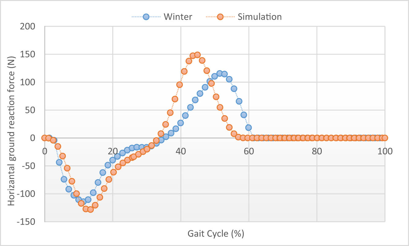
Comparison between model and healthy leg: HGRV vs gait cycle.

8 Conclusion

1. Kinematic and kinetic analyses of the prosthesis gait were effectively conducted in real-time operation by the event-based motion method, which gives a powerful tool for observing performance, the design of the gait process, and optimizing the properties of the prosthesis within its operating environment.

2. Two active motions were successfully used for simulating the motion of hip displacement and flexion/extension of the thigh during the gait cycle, which means that this simulation enables a computer-aided modeling environment to be developed for modeling sophisticated mechanical components.

3. The results found from both the simulation and the reference data showed good agreement, but there was some variations between the results due to the intricacy of the human joint and the simplicity of the intended mechanical joint. Predicted error levels occurred.

4. An important benefit of the simulation method is that it allows for evaluation prior to the amputee using the prosthesis. Also, the input data can be altered in response to the conditions that are applied, for instance, the patient’s height, the gait cycle features, and the kind of material of the prosthesis.

Future work is planned to develop the controller of the virtual model, which includes an interface between SolidWorks and LabVIEW or with Matlab to simulate the movement of the testing platform. Further work is required to adjust this virtual model to other types of the knee joint, such as the four-bar. Finally, the simulation model presented in this study can be viewed as the first stage toward a full virtual model.

References

[1] Hou Z, Chen H, Su J, Sui Z, Cui X, Tian Y. Design and implementation of high efficiency biped robot system. In: 2010 Chinese Control and Decision Conference. IEEE; 2010. p. 2433–8. 10.1109/CCDC.2010.5498809Suche in Google Scholar
[2] Collette C, Micaelli A, Andriot C, Lemerle P. Robust balance optimization control of humanoid robots with multiple non coplanar grasps and frictional contacts. In: 2008 IEEE International Conference on Robotics and Automation; 2008. p. 3187–93. 10.1109/robot.2008.4543696. Suche in Google Scholar
[3] Lien C-C, Tien C-C, Shih J-M. Human gait recognition for arbitrary view angles. In: Second International Conference on Innovative Computing, Informatio and Control (ICICIC 2007). IEEE; 2007. p. 303. 10.1109/icicic.2007.338. Suche in Google Scholar
[4] Culik J, Szabo Z, Krupicka R. Biomechanics of human gait simulation. In: World congress on medical physics and biomedical engineering. Berlin, Heidelberg: Springer; 2009. p. 1329–32. 10.1007/978-3-642-03882-2_352. Suche in Google Scholar
[5] Suzuki Y, Geyer H. A simple bipedal model for studying control of gait termination. Bioinspiration Biomimetics. 2018;13(3):036005. 10.1088/1748-3190/aaae8e. Suche in Google Scholar PubMed
[6] Ferreira JP, Crisostomo MM, Coimbra AP. Human gait acquisition and characterization. IEEE Trans. Instrument. Measurement. 2009;58(9):2979–88. 10.1109/tim.2009.2016801. Suche in Google Scholar
[7] Ramírez JF, Jaramillo Munoz E, Vélez JA. Algorithm for the prediction of the reactive forces developed in the socket of transfemoral amputees. Dyna. 2012;79(173):89–95. Suche in Google Scholar
[8] Winter DA. Biomechanics and motor control of human movement. Hoboken, New Jersey: John Wiley & Sons, Inc., 2009. 10.1002/9780470549148. Suche in Google Scholar
[9] Whittle MW. Gait analysis: An introduction. Edinburgh, New York: Butterworth-Heinemann; 2014. Suche in Google Scholar
[10] Borjian R. Design, modeling, and control of an active prosthetic knee. MSc thesis, University of Waterloo, Canada; 2008. Suche in Google Scholar
[11] Richter H, Simon D, Smith WA, Samorezov S. Dynamic modeling, parameter estimation and control of a leg prosthesis test robot. Appl Math Modell. 2015;39(2):559–73. 10.1016/j.apm.2014.06.006. Suche in Google Scholar
[12] Marinelli C, Giberti H, Resta F. Conceptual design of a gait simulator for testing lower-limb active prostheses. In: 2015 16th International Conference on Research and Education in Mechatronics (REM). IEEE; 2015. p. 314–20. 10.1109/rem.2015.7380413. Suche in Google Scholar
[13] Shandiz MA, Farahmand F, Osman NAA, Zohoor H. A robotic model of transfemoral amputee locomotion for design optimization of knee controllers. Int J Adv Robotic Syst. 2013;10(3):161. 10.5772/52855. Suche in Google Scholar
[14] Luengas Contreras LA, Camargo Casallas E, Guardiola D. Modelagem e simulacón da marcha protésica usando modelo em 3d de uma prótese transtibial. Revista Ciencias de la Salud. 2018;16(1):82. 10.12804/revistas.urosario.edu.co/revsalud/a.6492.Suche in Google Scholar
[15] Hoh S, Chong J, Etoundi AC. Design of a virtual testing platform for assessing prosthetic knee joints. In: 2020 5th International Conference on Advanced Robotics and Mechatronics (ICARM). 2020. p. 576–81. 10.1109/icarm49381.2020.9195275. Suche in Google Scholar
[16] Cao W, Yu H, Chen W, Meng Q, Chen C. Design and evaluation of a novel microprocessor-controlled prosthetic knee. IEEE Access. 2019;7:178553–62. 10.1109/access.2019.2957823. Suche in Google Scholar
[17] Asada H, Slotine J-J. Robot analysis and control. New York: John Wiley & Sons. 1991. Suche in Google Scholar
© 2022 Saif M. J. Haider et al., published by De Gruyter
This work is licensed under the Creative Commons Attribution 4.0 International License.
Artikel in diesem Heft
- Regular Articles
- Performance of a horizontal well in a bounded anisotropic reservoir: Part I: Mathematical analysis
- Key competences for Transport 4.0 – Educators’ and Practitioners’ opinions
- COVID-19 lockdown impact on CERN seismic station ambient noise levels
- Constraint evaluation and effects on selected fracture parameters for single-edge notched beam under four-point bending
- Minimizing form errors in additive manufacturing with part build orientation: An optimization method for continuous solution spaces
- The method of selecting adaptive devices for the needs of drivers with disabilities
- Control logic algorithm to create gaps for mixed traffic: A comprehensive evaluation
- Numerical prediction of cavitation phenomena on marine vessel: Effect of the water environment profile on the propulsion performance
- Boundary element analysis of rotating functionally graded anisotropic fiber-reinforced magneto-thermoelastic composites
- Effect of heat-treatment processes and high temperature variation of acid-chloride media on the corrosion resistance of B265 (Ti–6Al–4V) titanium alloy in acid-chloride solution
- Influence of selected physical parameters on vibroinsulation of base-exited vibratory conveyors
- System and eco-material design based on slow-release ferrate(vi) combined with ultrasound for ballast water treatment
- Experimental investigations on transmission of whole body vibration to the wheelchair user's body
- Determination of accident scenarios via freely available accident databases
- Elastic–plastic analysis of the plane strain under combined thermal and pressure loads with a new technique in the finite element method
- Design and development of the application monitoring the use of server resources for server maintenance
- The LBC-3 lightweight encryption algorithm
- Impact of the COVID-19 pandemic on road traffic accident forecasting in Poland and Slovakia
- Development and implementation of disaster recovery plan in stock exchange industry in Indonesia
- Pre-determination of prediction of yield-line pattern of slabs using Voronoi diagrams
- Urban air mobility and flying cars: Overview, examples, prospects, drawbacks, and solutions
- Stadiums based on curvilinear geometry: Approximation of the ellipsoid offset surface
- Driftwood blocking sensitivity on sluice gate flow
- Solar PV power forecasting at Yarmouk University using machine learning techniques
- 3D FE modeling of cable-stayed bridge according to ICE code
- Review Articles
- Partial discharge calibrator of a cavity inside high-voltage insulator
- Health issues using 5G frequencies from an engineering perspective: Current review
- Modern structures of military logistic bridges
- Retraction
- Retraction note: COVID-19 lockdown impact on CERN seismic station ambient noise levels
- Special Issue: Trends in Logistics and Production for the 21st Century - Part II
- Solving transportation externalities, economic approaches, and their risks
- Demand forecast for parking spaces and parking areas in Olomouc
- Rescue of persons in traffic accidents on roads
- Special Issue: ICRTEEC - 2021 - Part II
- Switching transient analysis for low voltage distribution cable
- Frequency amelioration of an interconnected microgrid system
- Wireless power transfer topology analysis for inkjet-printed coil
- Analysis and control strategy of standalone PV system with various reference frames
- Special Issue: AESMT
- Study of emitted gases from incinerator of Al-Sadr hospital in Najaf city
- Experimentally investigating comparison between the behavior of fibrous concrete slabs with steel stiffeners and reinforced concrete slabs under dynamic–static loads
- ANN-based model to predict groundwater salinity: A case study of West Najaf–Kerbala region
- Future short-term estimation of flowrate of the Euphrates river catchment located in Al-Najaf Governorate, Iraq through using weather data and statistical downscaling model
- Utilization of ANN technique to estimate the discharge coefficient for trapezoidal weir-gate
- Experimental study to enhance the productivity of single-slope single-basin solar still
- An empirical formula development to predict suspended sediment load for Khour Al-Zubair port, South of Iraq
- A model for variation with time of flexiblepavement temperature
- Analytical and numerical investigation of free vibration for stepped beam with different materials
- Identifying the reasons for the prolongation of school construction projects in Najaf
- Spatial mixture modeling for analyzing a rainfall pattern: A case study in Ireland
- Flow parameters effect on water hammer stability in hydraulic system by using state-space method
- Experimental study of the behaviour and failure modes of tapered castellated steel beams
- Water hammer phenomenon in pumping stations: A stability investigation based on root locus
- Mechanical properties and freeze-thaw resistance of lightweight aggregate concrete using artificial clay aggregate
- Compatibility between delay functions and highway capacity manual on Iraqi highways
- The effect of expanded polystyrene beads (EPS) on the physical and mechanical properties of aerated concrete
- The effect of cutoff angle on the head pressure underneath dams constructed on soils having rectangular void
- An experimental study on vibration isolation by open and in-filled trenches