A model for variation with time of flexiblepavement temperature

Miami M. Hilal; Mohammed Y. Fattah

doi:10.1515/eng-2022-0012

Article Open Access

A model for variation with time of flexiblepavement temperature

Miami M. Hilal and Mohammed Y. Fattah

Published/Copyright: March 16, 2022

Published by

Become an author with De Gruyter Brill

Submit Manuscript Author Information

From the journal Open Engineering Volume 12 Issue 1

Abstract

The bituminous material performance is affected basically by the prevailing temperatures. The mechanical properties of these materials can vary significantly with the changes in the temperature magnitude. Hot mix asphalt (HMA) is a visco-elastoplastic material, so the pavement structural capacity is affected by the temperature variations. To determine the characteristics of the strength of the flexible pavement rationally, the prediction of the distribution of temperature in HMA pavement layers is a must. Heavy loadings subjected to highways and roads can cause serious deterioration to the HMA pavements. In this research, the temperature for three thicknesses of asphalt pavement structure was measured, and the air temperature to predict a model explains the relationship between the temperature and the depth of the pavement structure. The suggested model was successfully validated utilizing the data from three depths of asphalt pavement structure and the temperature on the surface of the asphalt pavement. The developed model consists of two independent variables, which are the depth within the pavement and ambient air temperature. The predicted model will be useful for the pavement designers those in need to predict the temperature of the profile of pavement to determine the engineering characteristics of field pavement.

Keywords: asphalt pavements; layered system; air temperature; pavement temperature; temperature models

1 Introduction

From the initial Strategic Highway Research Program testing, the models of pavement temperature had been developed to support the selection of the adequate performance grade of asphalt binder to be used in a selected location [1,2,3,4].

Pavement temperature can be briefly defined as the changes in pavement surface temperature with the variation in weather parameters over time as influenced by the paving materials and direct solar reflectance, thermal conductivity, specific heat, and surface convection [5,6].

The temperature distribution is the most contributing environmental factor that affects the mechanical properties of flexible paving mixtures and the asphalt pavement structure’s bearing capacity [7].

The asphalt pavement performance is highly temperature sensitive [8]. Recently, summer temperature intends to be higher than any time before because of global warming, so different types of damages could occur in flexible pavements.

It has also been observed that the temperature in one section of an asphalt pavement varies due to several reasons. To better understand, pavement responses are affected primarily by ambient temperature, followed by solar radiation (during the hot season); the effect of wind speed and relative humidity, however, is less significant [9]. Thus, these parameters are considered as the necessary parameters in a pavement temperature prediction model [10]. Furthermore, extensive research on temperature prediction models has been conducted in several regions with different climates to formulate pavement temperature prediction models that provide the highest accuracy [8].

Several researchers have also raised their concern about temperature algorithms’ precision and the consequences of using predicted values by emerging technologies of deep learning-based regression models for calculating asphalt pavement temperature [11].

Solaimanian and Kennedy [12] predicted pavement temperatures through an analytical approach by using the theory of energy and heat transfer. Bosscher et al. [4] predicted models based on regression data sets. Marshall et al. [13] and Park et al. [14] also used the regression method to predict pavement temperature models. Hermansson [15,16] predicted a computer simulation model pavement temperatures in the summertime by using the heat transfer theoretical models given by Solaimanian and Kennedy. Some of the asphalt pavement temperature layer models can be predicted on an hourly/daily basis by using the statistical method [7].

Mohseni and Symons [17,18] predicted the temperature of asphalt pavement using a statistical model, and they concluded that minimum and maximum temperatures at different depths of asphalt pavement layer change with the variation of air and surface temperature linearly.

Diefenderfer Brian [19] determined the pavement temperature profile and the effects of cooling and heating trends within the pavement structure could be quantified; and showed that it could model the daily pavement minimum and maximum temperatures could be modeled by knowing the minimum or maximum ambient temperatures, the solar radiation, and the depth at which the temperature of pavement is desired, and extend the model to show that verification of the temperatures of pavement calculated by using the daily solar radiation could be applied to any location accurately.

Chao and Jinxi [20] used the method of partial least square to present a regression model by analyzing the collected data of the pavement temperature as well as the environmental data provided from the local weather station. As a result, the temperature of pavement can be estimated and predicted by the proposed model accurately and reliably.

Diefenderfer et al. [21] predicted models for the minimum daily and maximum daily pavement temperatures, which were developed and validated by using data from the Virginia Smart Road and two long-term pavement performance seasonal monitoring programs (LTPP SMP) test sites. The calculated pavement temperatures using the daily solar radiation could be applied to any location accurately.

The temperatures of asphalt pavement influence greatly the performance and bearing capacity, especially in the season of high temperature. The variation of pavement temperatures during the high temperature affects the structural design and the management of maintenance of the asphalt pavement layers and the estimation of pavement temperature models accurately. The temperature of asphalt pavement is affected greatly by many environmental factors and cannot be measured directly or predicted precisely.

The objective of the present work is to suggest a model for the prediction of pavement temperature in terms of pavement thickness and air temperature. The predicted model will be used by designers to predict the temperature of the profile of pavement to determine the engineering characteristics of field pavement. In this research work, sensors of temperature were buried or embedded in the pavement of a selected road to collect the data of temperature by continuously recorded measurement for 10 months. Then a model was predicted by using the regression analysis method using the SPSS program throughout a complete analysis on the recorded data of pavement temperature; the results showed that the temperature of pavement could be predicted by the model accurately and reliably.

2 Pavement temperature monitoring

Sensors of temperature were buried in the pavement structure to collect data of temperature for 10 months period from April 2018 till February 2019. The selected road is located in Baghdad city, which is used for collecting the data. The pavement structure of the selected site is composed of a surface layer, binder layer, base layer, sub-base layer, and subgrade, as shown in Figure 1(a). Data were collected by using a temperature data logger device that has high-quality thermostat sensors from −40 to +85°C and it is composed of four channels; three of them were used for collecting the temperature data of the three depths of asphalt pavement for model development: 2.0, 7.0, and 10.0 cm below the pavement surface, and the fourth one for air temperature. All three depths were located within the hot mix asphalt (HMA) layer. The accuracy of the memory of the device is 0.25% for 12 bit resolution, and 8 bit or 10 bit resolution can also be set to maximize memory usage.

Figure 1

(a) Pavement structure layers. (b) Data logger device.

Temperature data are recorded in the device daily and hourly in EXCEL sheet and could be drawn from the device for each desired period as presented in Figure 2, which shows the temperature values for 13–25 May 2018 each hour of the day for the three depths and the air temperature values.

Figure 2

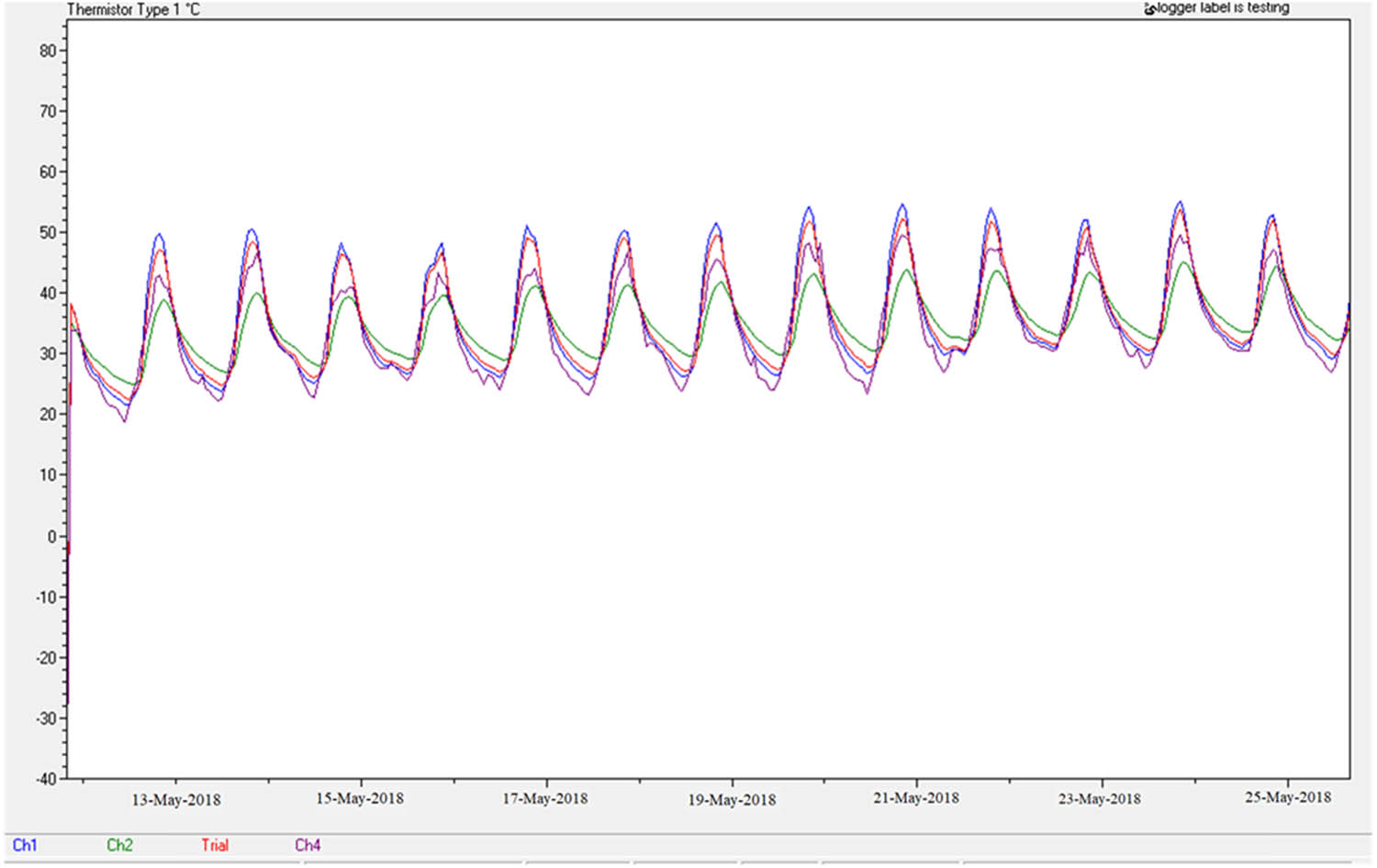
Relationship of temperature values with time from data logger software.

2.1 Effect of air temperature

Figure 3 presents the relationship between the air temperature and time measured on Friday, 15 January 2019. The figure shows that during the daytime, the temperature rises until it reaches a maximum value with time and decreases during the night till reaching a minimum value.

Figure 3

Relationship between air temperature and time.

2.2 Effect of temperature on asphalt pavement layers

Figure 4 presents an example of the relationship between the temperature and time measured at different asphalt pavement layer depths; 0, 2, 7, and 10 cm from the surface during Friday, 15 January 2019, whereas Table 1 presents the maximum and minimum values of temperature for all layers during that day. As shown in the figure, the temperature rises during the day and decreases during the night because of the heat of the sun. As presented in the figure, it is clear that at midnight (i.e. time = 0) the value of temperature at the surface has the lowest value, whereas at 10 cm below the surface the value of temperature is the maximum value. The values of temperature at all the layers decrease at night and continue to decrease till they reach the minimum value before the rise of the sun. The value of temperature will increase at the surface layer when the sun rises and the ambient temperature increases; also, the temperature will be transferred to the second layer and will continue to transfer throughout the layers during the day. As presented in the figure, at midday (i.e. time = 12) the surface temperature is equal to the value of temperature at 10 cm, and the values of temperature continue to increase till reaching their maximum value at all layers. When the sun begins to set (i.e. time = 17), the value of temperature at the surface will begin to decrease as well as at all layers. The figure also shows that the temperature increases as the depth of the pavement decrease during the day, whereas it increases with the increase of the pavement depths during the night. That is because of temperature dispersion throughout the pavement layers.

Table 1

The minimum and maximum values of temperature (°C) for all layers on Friday, 15 January 2019

Layer depth (cm)	Temperature value (°C)
Layer depth (cm)	Minimum	Time	Maximum	Time
0	12.6	06:48:37	20.7	17:48:37
2	12.8	10:48:37	20.7	17:48:37
7	13.2	11:48:37	19.6	18:48:37
10	14.6	11:48:37	18.3	19:48:37

Figure 4

Relationship between the temperature and asphalt pavement thickness.

2.3 Regression analysis and model development

After data collection, the program used for predicting the model of pavement temperature was SPSS.

2.4 Regression analysis

It is a statistical technique that attempts to explain and design the relationship between dependent and independent variables. The dependent variable is pavement temperature (T _pav., °C), whereas the independent variables are the thickness of pavement (h, cm) and air temperature (T _air, °C).

To build the model, the number of samples must be checked. T-test was used to determine whether to use 50 or 75% of samples make a difference in the results. Table 2 shows the T-test results for each pair of samples.

Table 2

Paired samples T-test

Pair of samples	Paired differences					t	df	Sig. (2-tailed)
	Mean	Std. seviation	Std. error mean	95% confidence interval of the difference
	Mean	Std. seviation	Std. error mean	Lower	Upper
50 and 75%	−0.149	20.267	0.196	−0.534	0.234	−0.763	10,665	0.445

From Table 2 the t-test results show that using 50% of samples or 75% of samples does not make any difference because significant 2-tailed is greater than 0.05 confidence level.

Around 75% of the collected data were selected randomly by the SPSS program and used for building the model, whereas 25% of the data were used for model validation. Table 3 presents the correlation matrix between the dependent and independent variables.

Table 3

Correlation matrix between dependent and independent variables

Correlations
		T _pav.	h	T _air
T _pav	Pearson correlation	1	0.014	0.971**
	Sig. (2-tailed)		0.073	0.000
	N	15,722	15,722	15,722
h	Pearson correlation	0.014	1	−0.001
	Sig. (2-tailed)	0.073		0.880
	N	15,722	15,722	15,722
T _air	Pearson correlation	0.971**	−0.001	1
	Sig. (2-tailed)	0.000	0.880
	N	15,722	15,722	15,722

**Correlation is significant at the 0.01 level (2-tailed).

2.5 Model limitations

Table 4 presents the limitations of the data used to build and validate the model.

Table 4

Data limitations used in the model

Variable	Range	Min.	Max.	Mean
Building model data, sample size = 15,722
T _pav.	55	3.2	58.2	29.142
h	8	2	10	6.330
T _air	53.5	2.6	56.1	27.6
Validation data, sample size = 5,248
T _pav.	54.3	3.2	57.5	29.041
h	8	2	10	6.343
T _air	53.1	2.6	55.7	27.520

3 Measurement of fit goodness

The measurement of fit goodness is focused on the evaluation of how the predicted regression model is well-fitting the collected data. The two coefficients of measures that are presented are the determination coefficient (R ²) and standard error of the regression (SER). Several statisticians used the adjusted multiple determinations coefficient, adjusted R, which refers to the magnitude increase of R when a new parameter enters the model. The SER parameter can be found by the following relationship:

(1) SER = SSE n − ( k + 1 ) 0.5 ,

where SSE = sum squares of error ∑ ( y i − y i ′ ) 2 , y i = the actual response value variable for the ith case. y i ′ = the regression prediction value for the ith case. n − ( k + 1 ) = degree of freedom (d_f). n = sample number, and k = independent variables number.

The analysis of variance (ANOVA) results and summary of the regression analysis for the model are presented in Tables 5 and 6.

Table 5

ANOVA results for pavement temperature model

ANOVA^b
Model		Squares sum	d _f	Mean square	F	Significant
1	Regression value	1909796.126	2	954898.063	131156.980	0.000^a
	Residual value	114443.338	15,719	7.281
	Total	2024239.464	15,721

a. Predictors: (constant), T _air, thickness. b. Dependent variable: T _pav.

Table 6

Developed model summary

Summary of model
Model	R	R ²	Adjusted R ²	Estimate std. error
1	0.971^a	0.943	0.943	2.698

a. Predictors: (constant), T _air, thickness.

From the ANOVA table results, the F statistic is the regression mean square divided by the residual mean square. The significance value of the F statistic is smaller than 0.05 for the developed model; then, the independent variables are explain the variation in the dependent variable significantly.

The analysis of results and calculation of correlation coefficient (R), coefficient of determination (R ²), and standard regression error for the developed model are calculated and presented in Table 5. The determination coefficient (R ²) is (0.943); this is the mean that there is only 5.7% of the observed variation is unexplained by the predicted model. That leads to a very good correlation between the measured and predicted values of pavement temperature (T _pav.).

4 Discussion of regression analysis results

To know the effect of the independent variables (pavement thickness (h) and air temperature (T _air)) on the dependent variable pavement temperature (T _pav.), the multiple regression analysis was used.

From the SPSS program, the model of pavement temperature was predicted and the model description was as follows and can be seen in Table 7:

(2) T pav . = 1.521 + 0.053 h + 0.988 T air .

Table 7

Regression of developed model

		Model coefficients^a
		Unstandardized coefficients		Standardized coefficients	t-value	Significant
Model		B	Standard error	Beta	t-value	Significant
1	(Constant)	1.521	0.071		21.484	0.000
	h	0.053	0.007	0.015	8.145	0.000
	T _air	0.988	0.002	0.971	512.111	0.000

a. Dependent variable: T _pav.

It is clear from the values of beta value which is the standardized coefficient, the air temperature (T _air) independent variable is highly affecting in the estimation of the temperature of pavement which is the dependent variable (T _pav.) because the beta value is the highest one (0.971), whereas for the second independent variable the thickness of pavement (h), the beta value is (0.015) which has the lowest effect in the estimation of the (T _pav.). A significant level is less than 0.05 for all independent variables, as presented in Table 7.

5 Predicted model validation

The validation process is to evaluate the adequacy of the predicted model and measurement of the accuracy or error of the estimation for the period of validation.

Excel software was used to validate the model. A total of 25% of the data which have not been used for building the model were used in the validation process. Figure 5 presents the relationship between the estimated (developed) and the actual pavement temperature (T _pav.). As shown in the figure, the correlation coefficient (R) value is 0.972; thus, the developed model is considered to be valid.

Figure 5

Actual versus estimated pavement temperature (T _pav.).

It is worth mentioning that the properties of asphalt binder/mixture, especially those related to temperature, can be enhanced with the addition of polymers such as waste polypropylene, especially for high-temperature regions. Polymers would decrease the negative environmental effects, as concluded by Abdulkhabeer et al. [22].

6 Conclusions

The following can be concluded:

The temperature has a relatively significant impact on the physical and mechanical material properties of the asphalt pavement layer.
A model for predicting the pavement temperature was developed and validated using data from a selected site in Baghdad city, the capital of Iraq. The developed model consists of two independent variables, which are the depth within the pavement and ambient air temperature as follows:
T pav . = 1.521 + 0.053 h + 0.988 T air .
The predicted model (T _pav.) will be useful for the pavement designers those in need to predict the temperature of the profile of pavement to determine the engineering characteristics of field pavement.
The model may be applied for estimating the performance of rutting, which is a result of heavy vehicle loading. Also, it may be applied for estimating the low-temperature cracking of HMA pavements.
The model can predict the future pavement temperatures (T _pav.) using the trends of ambient temperature from previously recorded data, and that will be useful for researchers in estimating the total time that pavements are subjected to critical temperatures.

7 Recommendations

It is recommended to

Carry out additional research on this topic and include other variables in predicting the model of pavement temperatures like seasonal effects, amplitude, and solar radiation to produce the profiles of real-time pavement temperature and heat transfer between the environmental and pavement temperatures.
Determine pavement temperature profile models for maximum and minimum ambient temperatures with depth.

Conflict of interest: Authors state no conflict of interest.

References

[1] Mohseni A, Symons M. Improved AC pavement temperature models from LTPP seasonal data. Presented at Transportation Research Board 77th Annual Meeting. Washington, DC; 1998a.Search in Google Scholar

[2] Mohseni A, Symons M. Effect of improved LTPP AC pavement temperature models on SuperPave performance grades. Presented at Transportation Research Board 77th Annual Meeting. Washington, DC; 1998b.Search in Google Scholar

[3] Lukanen EO, Han C, Skok, Jr EL. Probabilistic method of asphalt binder selection based on pavement temperature. Transportation research record 1609. Washington, DC: TRB, National Research Council; 1998. p. 12–20.10.3141/1609-02Search in Google Scholar

[4] Bosscher PJ, Bahia HU, Thomas S, Russell JS. Relationship between pavement temperature and weather data: wisconsin field study to verify SuperPave algorithm. Transportation research record 1609, TRB. Washington, DC: National Research Council; 1998. p. 1–11.10.3141/1609-01Search in Google Scholar

[5] Nižetíc S, Papadopoulos A. The role of exergy in energy and the environment. Cham, Switzerland: Springer International Publishing; 2018. ISBN 978-3-319-89844-5.10.1007/978-3-319-89845-2Search in Google Scholar

[6] Van Dam TJ, Harvey JT, Muench ST, Smith KD, Snyder MB, Al-Qadi IL et al. Towards sustainable pavement systems. Urbana, IL, USA: Applied Pavement Technology Inc.; 2015.Search in Google Scholar

[7] Adwan I, Milad A, Memon ZA, Widyatmoko I, Ahmat Zanuri N, Memon NA, et al. Asphalt pavement temperature prediction models: a review. Appl Sci J. 2021;11:3794. 10.3390/app1109379.Search in Google Scholar

[8] Sun L, Qin J. Prediction model on temperature field in asphalt pavement. J Tongji Univ. 2006;34(4):480–3.Search in Google Scholar

[9] Salem HA. Research of the relevant temperatures for the design of pavement constructions on the desert roads in Libya. Novi Sad, Serbia: Faculty of Technical Sciences, University of Novi Sad; 2015.Search in Google Scholar

[10] Dong W. Simplified analytical approach to predicting asphalt pavement. J Mater Civ Eng. 2016;27:864–70.10.1061/(ASCE)MT.1943-5533.0000826Search in Google Scholar

[11] Milad A, Adwan I, Majeed SA, Yusoff NIM, Al-Ansari N, Yaseen ZM. Emerging technologies of deep learning models development for pavement temperature prediction. IEEE Access. 2021;9:23840–49.10.1109/ACCESS.2021.3056568Search in Google Scholar

[12] Solaimanian M, Kennedy TW. Predicting maximum pavement surface temperature using maximum air temperature and hourly solar radiation. Transportation research record 1417, TRB. Washington, DC:; National Research Council; 1993. p. 1–11.Search in Google Scholar

[13] Marshall C, Meier RW, Welsh M. Seasonal temperature effects on flexible pavements in tennessee. Presented at Transportation Research Board 80th Annual Meeting. Washington, DC; 2001.10.3141/1764-10Search in Google Scholar

[14] Park D, Buch N, Chatti K. Development of effective layer temperature prediction model and temperature correction using FWD deflections. Presented at Transportation Research Board 80th Annual Meeting. Washington, DC; 2001.10.3141/1764-11Search in Google Scholar

[15] Hermansson A. Simulation model for calculating pavement temperatures, including maximum temperature. Transportation research record 1699. Washington DC: Transportation Research Board; 2000. p. 134–41.10.3141/1699-19Search in Google Scholar

[16] Hermansson A. A mathematical model for calculating pavement temperatures, comparisons between calculated and measured temperatures. Proceedings Transportation Research Board 80th Annual Meeting, CD-ROM. Washington, D.C: Transportation Research Board; 2001.10.3141/1764-19Search in Google Scholar

[17] Mohseni A, Symons M. Effect of improved LTPP AC pavement temperature models on superpave performance grades. Proceedings of 77th Annual TRB Conference. Washington, DC, USA; 1998.Search in Google Scholar

[18] Mohseni A, Symons M. Improved ad pavement temperature models from LTPP seasonal data. Proceedings of 77th Annual Transportation Research Board (TRB) Conference. Washington, DC, USA; 1998.Search in Google Scholar

[19] Diefenderfer Brian K, Al-Qadi Imad L, Reubush Stacey D, Freeman Thomas E. Prediction of Daily Temperature Profile in Flexible Pavements at Multiple Locations Using LTPP Data. TRB Annual Meeting; 2003.Search in Google Scholar

[20] Chao J, Jinxi Z. Prediction Model for Asphalt Pavement Temperature in High-Temperature Season in Beijing. 11, Hindawi: Advances in Civil Engineering; 2018. p. 1837952. 10.1155/2018/1837952.Search in Google Scholar

[21] Diefenderfer BK, Al-Qadi IL, Diefenderfer SD. Model to predict pavement temperature profile: development and validation. J Trans Eng, ASCE/February. 2006;132(2):162–7. 10.1061/_ASCE_0733-947X_2006_132:2_162.Search in Google Scholar

[22] Abdulkhabeer WN, Fattah MY, Hilal MM. Characteristics of asphalt binder and mixture modified with waste polypropylene. Eng Technol J. 2021;39(08):1224–30. 10.30684/etj.v39i8.1716.Search in Google Scholar

Received: 2021-09-11

Revised: 2022-01-06

Accepted: 2022-01-16

Published Online: 2022-03-16

This work is licensed under the Creative Commons Attribution 4.0 International License.

Articles in the same Issue

https://doi.org/10.1515/eng-2022-0012

Keywords for this article

asphalt pavements; layered system; air temperature; pavement temperature; temperature models

Creative Commons

BY 4.0