Performance of a horizontal well in a bounded anisotropic reservoir: Part I: Mathematical analysis

Timothy Kitungu Nzomo; Stephen Ezizanami Adewole; Kennedy Otieno Awuor; Daniel Okang’a Oyoo

doi:10.1515/eng-2022-0003

Article Open Access

Performance of a horizontal well in a bounded anisotropic reservoir: Part I: Mathematical analysis

Timothy Kitungu Nzomo , Stephen Ezizanami Adewole , Kennedy Otieno Awuor and Daniel Okang’a Oyoo

Published/Copyright: February 7, 2022

Published by

Become an author with De Gruyter Brill

Submit Manuscript Author Information

From the journal Open Engineering Volume 12 Issue 1

Abstract

To enhance the productivity of horizontal wells, it is of necessity to ensure that they perform optimally. This requires an understanding of how the reservoir’s geometry, anisotropy and well design affect the pressure response. Mathematical formulations can be used to simulate pressure response in the wellbore and the data obtained can be analysed to obtain well and reservoir parameters that can aid performance and evaluation. In this study, a mathematical model that can be used to approximate pressure response in a horizontal well is formulated, and a detailed mathematical analysis that can be used to obtain well and reservoir parameters are provided. A horizontal well inside a rectangular drainage volume with sealed boundaries is considered and the effect of each boundary on pressure throughout its productive life is studied. In the analysis, investigations on how the reservoir parameters can be approximated over a given period of production are conducted. This is achieved by identification of the appropriate source and Green’s functions. These source functions allow us to formulate a mathematical model for dimensionless pressure. Considering the diagnostic plots for both dimensionless pressure and dimensionless pressure derivative, mathematical analysis studies the possible behaviour of the plots. Analysis indicates that the reservoir anisotropy can be approximated during the infinite-acting flow at early times when other parameters are known. Further, when the first boundary is felt, in this case the vertical boundary, the horizontal permeability can be approximated during the transition flow periods at middle times. Finally, at late times when all the boundaries have been felt and a pseudosteady state flow is evident, reservoir dimensions can be approximated. These results can significantly improve well test analysis and enhance the performance evaluation of a horizontal well.

Keywords: horizontal wells; pseudosteady state flow; reservoir geometry; anisotropy; pressure response

1 Introduction

Horizontal wells are replacing vertical wells in modern exploration of oil due to their improved production over a given drainage volume. Their ability to reach larger areas of a drainage volume places them at an advantage compared to vertical wells. With their drilling complexity, this comes with more cost and thus it is important that proper evaluation and a good understanding of their performance is improved so that they can be more productive. The length of the well to be drilled in a given drainage volume so as to maximise the pressure response is of importance compared to the dimensions of the reservoir. Mathematical models are used to simulate pressure response and thus can be used to analyse the data obtained from well tests.

In a monograph [1], the advances in well test analysis with discussions on the use of diffusivity equation in solving fluid flows are discussed. The pressure behaviour during infinite-acting flow is discussed in detail in ref. [2], in which, the exponential integral is applied in the approximation of pressure. In a very detailed paper [3], instantaneous source and Green’s functions are studied and it is demonstrated that a solution of the diffusivity equation could be obtained using the product of the appropriate source and Green’s functions when the Newman’s product method was used. This provided a way of solving unsteady flows. In refs [4–8], studies using these source and Green’s functions were conducted and mathematical models which could simulate pressure response in reservoirs were developed. In these studies, infinite-acting models are considered, with some considering certain boundaries as sealed. Isotropic cases were employed in most studies to simplify calculations, thus not considering each directional permeability. These approximations and assumptions continue to limit the models and affect the accuracy of the results obtained. In an attempt to delineate flow periods, authors [9,10] developed strategies of delineating flow periods and developed equations that could be used to approximate the time when flow periods started or ended in a rectangular drainage system. With more horizontal wells being drilled, it became even more necessary to account for these flow periods and how the pressure response during a certain flow period was affected by the well design and the reservoir geometry. This has seen development of more models to simulate pressure response and investigate how well and reservoir parameters influence the performance of a horizontal well. Source and Green’s functions have been considered further in the development of these models. Authors [11–20] have developed models and used them to study horizontal well performance. The consideration of only the infinite-acting flow, sealing of certain boundaries and isotropic cases to ease the complexity of anisotropy considerations in three dimensional drainage volumes continue to limit these models. In this study, the performance of a horizontal well in an anisotropic reservoir when all the boundaries are sealed is investigated.

2 Reservoir physical model description

A completely sealed rectangular drainage volume of dimensionless length, x _eD, dimensionless width, y _eD and dimensionless thickness, h _D is considered. A horizontal well of dimensionless length, L _D drilled in the x-direction is considered. For mathematical analysis, the well is considered to be parallel to the x-boundary and perpendicular to the y-boundary. The well is centrally located in the reservoir such that from the centre of the reservoir located at (x _wD, y _wD, z _wD), the well stretches to a length L _D/2 in both the directions along the x-axis as shown in Figure 1.

Figure 1

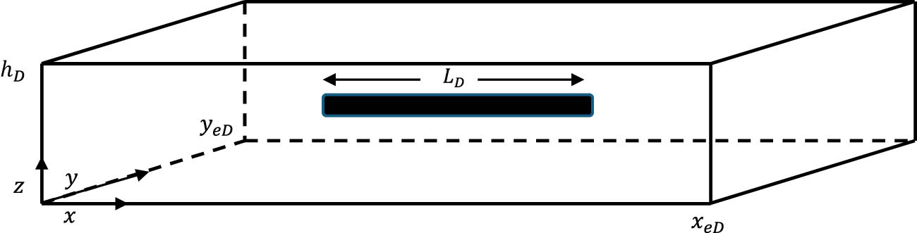
Horizontal well in a rectangular drainage volume.

3 Mathematical description

The heterogeneous three dimensional diffusivity equation accounting for directional permeability as given by ref. [9] is shown in equation (1),

(1) k x ∂ 2 P ∂ x 2 + k y ∂ 2 P ∂ y 2 + k z ∂ 2 P ∂ z 2 = Φ μ c t ∂ P ∂ t ,

Where k _x, k _y and k _z are the axial permeabilities in x, y and z directions, Φ is porosity, μ is reservoir fluid viscosity, c _t is total compressibility and P is pressure.

Equation (1) finds a lot of applications in solving unsteady flows and its solution for dimensionless pressure P _D as given by ref. [11] is shown in equation (2), and the dimensionless pressure derivative P D ′ is given by equation (3):

(2) P D = 2 π h D ∫ 0 t D s ( x D , τ D ) ⋅ s ( y D , τ D ) ⋅ s ( z D , τ D ) d τ D ,

(3) P D ′ = t D ∂ P D ∂ t D ,

where t _D is dimensionless time and τ _D is a dummy variable for time.

In equation (2), s(i _D, τ _D) is the appropriate instantaneous source and Green’s function in the respective axial direction given by:

An infinite-slab source of thickness L located at x = x _w in an infinite-slab reservoir given by ref. [3] and simplified by inserting dimensionless variables is approximated as shown in equation (4) at early time and as shown in equation (5) for late time.
(4) s ( x D , t D ) = 1 2 erf k / k x + ( x D − x w D ) 2 t D + erf k / k x + ( x D − x w D ) 2 t D ,

(5) s ( x D , t D ) = 1 x e D 1 + 2 x e D π ∑ n = 1 ∞ 1 n exp − n 2 π 2 t D x e D 2 × sin n π x e D cos n π x w D x e D cos n π x D x e D ,
An infinite plane-source located at y = y _w in an infinite-slab reservoir of thickness y _e given by ref. [3] and simplified by inserting dimensionless variables is approximated as shown in equation (6) at early time and as shown in equation (7) for late time.
(6) s ( y D , t D ) = 1 2 π t D k k y exp − ( y D − y w D ) 2 4 t D ,

(7) s ( y D , t D ) = 1 y e D 1 + 2 ∑ m = 1 ∞ exp − m 2 π 2 t D y e D 2 × cos m π y w D y e D cos m π y D y e D ,
An infinite plane-source at z = z _w in an infinite-slab reservoir of thickness h given by ref. [3] and simplified by inserting dimensionless variables is approximated as shown in equation (8) at early time and as shown in equation (9) for late time.

(8) s ( z D , t D ) = 1 2 π t D k k z exp − ( z D − z w D ) 2 4 t D ,

(9) s ( z D , t D ) = 1 h D 1 + 2 ∑ l = 1 ∞ exp − l 2 π 2 t D h D 2 cos l π z w D h D cos l π z D h D ,

Substituting these instantaneous source and Green’s functions in equation (2), solving for equation (3) and simplifying, we obtain the following mathematical models to simulate dimensionless pressure response at early time as reported in ref. [21];

During infinite-acting flow when no boundary has been felt, the dimensionless pressure is given by equation (10) and the dimensionless pressure derivative by equation (11).
(10) P D = − β h D k 4 k y k z Ei − r w D 2 4 t D e ,

(11) P D ′ = β h D k 4 k y k z exp − r w D 2 4 t D e ,
where r _wD is defined by equation (12).
(12) r w D 2 = ( y D − y w D ) 2 + ( z D − z w D ) 2 .

The exponential integral Ei(−x) in equation (10) is defined as
(13) Ei ( − x ) = − ∫ x ∞ e − u u d u ,
When the vertical boundary is felt, the dimensionless pressure is given by equation (14) and the dimensionless pressure derivative by equation (15).
(14) P D = π 2 k k y ∫ t D e t D 1 erf k / k x + ( x D − x w D ) 2 τ D + erf k / k x − ( x D − x w D ) 2 τ D × exp − ( y D − y w D ) 2 4 τ D × 1 + 2 ∑ l = 1 ∞ exp − l 2 π 2 τ D h D 2 cos l π z w D h D cos l π z D h D d τ D τ D ,

(15) P D ′ = π 2 k k y erf k / k x + ( x D − x w D ) 2 t D + erf k / k x − ( x D − x w D ) 2 t D × exp − ( y D − y w D ) 2 4 t D × 1 + 2 ∑ l = 1 ∞ exp − l 2 π 2 t D h D 2 cos l π z w D h D cos l π z D h D t D ,
When the horizontal boundary parallel to the well is felt before the horizontal perpendicular boundary, the dimensionless pressure is given by equation (16) and the dimensionless pressure derivative by equation (17).
(16) P D = π y e D ∫ t D 1 t D 2 erf k / k x + ( x D − x w D ) 2 τ D + erf k / k x + ( x D − x w D ) 2 τ D ⋅ 1 + 2 ∑ m = 1 ∞ exp − m 2 π 2 τ D y e D 2 cos m π y w D y e D cos m π y D y e D ⋅ 1 + 2 ∑ l = 1 ∞ exp − l 2 π 2 τ D h D 2 cos l π z w D h D cos l π z D h D d τ D ,

(17) P D ′ = π y e D erf k / k x + ( x D − x w D ) 2 t D + erf k / k x + ( x D − x w D ) 2 t D ⋅ 1 + 2 ∑ m = 1 ∞ exp − m 2 π 2 t D y e D 2 cos m π y w D y e D cos m π y D y e D ⋅ 1 + 2 ∑ l = 1 ∞ exp − l 2 π 2 t D h D 2 cos l π z w D h D cos l π z D h D t D ,
In case the horizontal boundary perpendicular to the well is felt before the horizontal parallel boundary, dimensionless pressure is given by equation (18) and the dimensionless pressure derivative by equation (19).

(18) P D = π x e D k k y ∫ t D 1 t D 2 1 + 2 x e D π ∑ n = 1 ∞ 1 n exp − n 2 π 2 τ D x e D 2 × sin n π x e D cos n π x w D x e D cos n π x D x e D × exp − ( y D − y w D ) 2 4 τ D 1 + 2 ∑ l = 1 ∞ exp − l 2 π 2 τ D h D 2 × cos l π z w D h D cos l π z D h D d τ D τ D ,

(19) P D ′ = π x e D k k y 1 + 2 x e D π ∑ n = 1 ∞ 1 n exp − n 2 π 2 t D x e D 2 × sin n π x e D cos n π x w D x e D cos n π x D x e D × exp − ( y D − y w D ) 2 4 t D 1 + 2 ∑ l = 1 ∞ exp − l 2 π 2 t D h D 2 × cos l π z w D h D cos l π z D h D t D ,

When all the boundaries have been felt and a pseudosteady state behaviour is evident, the dimensionless pressure is given by equation (20) and the dimensionless pressure derivative by equation (21) as reported in ref. [22].

(20) P D = 2 π x e D y e D ∫ t D 2 t D 1 + 2 x e D π ∑ n = 1 ∞ 1 n exp − n 2 π 2 t D x e D 2 × sin n π x e D cos n π x w D x e D cos n π x D x e D ⋅ 1 + 2 ∑ m = 1 ∞ exp − m 2 π 2 t D y e D 2 cos m π y w D y e D cos m π y D y e D ⋅ 1 + 2 ∑ l = 1 ∞ exp − l 2 π 2 t D h D 2 cos l π z w D h D cos l π z D h D d τ D ,

(21) P D ' = 2 π x e D y e D 1 + 2 x e D π ∑ n = 1 ∞ 1 n exp − n 2 π 2 t D x e D 2 × sin n π x e D cos n π x w D x e D cos n π x D x e D ⋅ 1 + 2 ∑ m = 1 ∞ exp − m 2 π 2 t D y e D 2 cos m π y w D y e D cos m π y D y e D ⋅ 1 + 2 ∑ l = 1 ∞ exp − l 2 π 2 t D h D 2 cos l π z w D h D cos l π z D h D t D .

In this study, the performance of the well from inception to date is considered. To determine the dimensionless pressure response from inception to date, the pressure response models from the infinite-acting flow when no boundary has been felt, through the transition flows as specific boundaries are felt up to the point when all the boundaries are felt and a pseudosteady state flow is evident are superposed. Since the formation thickness is considered far much smaller compared to the length and width of the reservoir, it is expected that the vertical boundary will be felt earlier than the horizontal boundaries. Depending on which of the two horizontal boundaries is felt earlier after the vertical boundary has been felt, the mathematical model for computing dimensionless pressure and its dimensionless pressure derivative starting from inception to date will have two cases. First, for a case where the horizontal boundary parallel to the well (y-boundary) is felt first, dimensionless pressure is given by equation (22) and the dimensionless pressure derivative by equation (23).

(22) P D = − β h D k 4 k y k z Ei − r w D 2 4 t D e + π 2 k k y ∫ t D e t D 1 erf k / k x + ( x D − x w D ) 2 τ D + erf k / k x − ( x D − x w D ) 2 τ D exp − ( y D − y w D ) 2 4 τ D 1 + 2 ∑ l = 1 ∞ exp − l 2 π 2 τ D h D 2 cos l π z w D h D cos l π z D h D d τ D τ D + π y e D ∫ t D 1 t D 2 erf k / k x + ( x D − x w D ) 2 τ D + erf k / k x + ( x D − x w D ) 2 τ D ⋅ 1 + 2 ∑ m = 1 ∞ exp − m 2 π 2 τ D y e D 2 cos m π y w D y e D cos m π y D y e D ⋅ 1 + 2 ∑ l = 1 ∞ exp − l 2 π 2 τ D h D 2 cos l π z w D h D cos l π z D h D d τ D + 2 π x e D y e D ∫ t D 2 t D 1 + 2 x e D π ∑ n = 1 ∞ 1 n exp − n 2 π 2 τ D x e D 2 sin n π x e D cos n π x w D x e D cos n π x D x e D ⋅ 1 + 2 ∑ m = 1 ∞ exp − m 2 π 2 τ D y e D 2 cos m π y w D y e D cos m π y D y e D ⋅ 1 + 2 ∑ l = 1 ∞ exp − l 2 π 2 τ D h D 2 cos l π z w D h D cos l π z D h D d τ D ,

(23) P D ′ = β h D k 4 k y k z exp − r w D 2 4 t D + π 2 k k y erf k / k x + ( x D − x w D ) 2 t D + erf k / k x − ( x D − x w D ) 2 t D exp − ( y D − y w D ) 2 4 t D 1 + 2 ∑ l = 1 ∞ exp − l 2 π 2 t D h D 2 cos l π z w D h D cos l π z D h D t D + π y e D erf k / k x + ( x D − x w D ) 2 t D + erf k / k x + ( x D − x w D ) 2 t D ⋅ 1 + 2 ∑ m = 1 ∞ exp − m 2 π 2 t D y e D 2 cos m π y w D y e D cos m π y D y e D ⋅ 1 + 2 ∑ l = 1 ∞ exp − l 2 π 2 t D h D 2 cos l π z w D h D cos l π z D h D t D + 2 π x e D y e D 1 + 2 x e D π ∑ n = 1 ∞ 1 n exp − n 2 π 2 t D x e D 2 sin n π x e D cos n π x w D x e D cos n π x D x e D ⋅ 1 + 2 ∑ m = 1 ∞ exp − m 2 π 2 t D y e D 2 cos m π y w D y e D cos m π y D y e D ⋅ 1 + 2 ∑ l = 1 ∞ exp − l 2 π 2 t D h D 2 cos l π z w D h D cos l π z D h D t D .

Second, the horizontal boundary perpendicular to the well (x-boundary) is felt first. In this case, the dimensionless pressure is given by equation (24) and dimensionless pressure derivative given by equation (25).

(24) P D = − β h D 4 k k k y k z Ei − r w D 2 4 t D e + π 2 k k y ∫ t D e t D 1 erf k / k x + ( x D − x w D ) 2 τ D + erf k / k x − ( x D − x w D ) 2 τ D exp − ( y D − y w D ) 2 4 τ D 1 + 2 ∑ l = 1 ∞ exp − l 2 π 2 τ D h D 2 cos l π z w D h D cos l π z D h D d τ D τ D + π x e D k k y ∫ t D 1 t D 2 1 + 2 x e D π ∑ n = 1 ∞ 1 n exp − n 2 π 2 τ D x e D 2 sin n π x e D cos n π x w D x e D cos n π x D x e D exp − ( y D − y w D ) 2 4 τ D × 1 + 2 ∑ l = 1 ∞ exp − l 2 π 2 τ D h D 2 cos l π z w D h D cos l π z D h D d τ D τ D + 2 π x e D y e D ∫ t D 2 t D 1 + 2 x e D π ∑ n = 1 ∞ 1 n exp − n 2 π 2 τ D x e D 2 sin n π x e D cos n π x w D x e D cos n π x D x e D ⋅ 1 + 2 ∑ m = 1 ∞ exp − m 2 π 2 τ D y e D 2 cos m π y w D y e D cos m π y D y e D ⋅ 1 + 2 ∑ l = 1 ∞ exp − l 2 π 2 τ D h D 2 cos l π z w D h D cos l π z D h D d τ D ,

(25) P D ′ = β h D 4 k k k y k z exp − r w D 2 4 t D + π 2 k k y erf k / k x + ( x D − x w D ) 2 t D + erf k / k x − ( x D − x w D ) 2 t D exp − ( y D − y w D ) 2 4 t D 1 + 2 ∑ l = 1 ∞ exp − l 2 π 2 t D h D 2 cos l π z w D h D cos l π z D h D t D + π x e D k k y 1 + 2 x e D π ∑ n = 1 ∞ 1 n exp − n 2 π 2 t D x e D 2 sin n π x e D cos n π x w D x e D cos n π x D x e D exp − ( y D − y w D ) 2 4 t D × 1 + 2 ∑ l = 1 ∞ exp − l 2 π 2 t D h D 2 cos l π z w D h D cos l π z D h D t D + 2 π x e D y e D 1 + 2 x e D π ∑ n = 1 ∞ 1 n exp − n 2 π 2 t D x e D 2 sin n π x e D cos n π x w D x e D cos n π x D x e D ⋅ 1 + 2 ∑ m = 1 ∞ exp − m 2 π 2 t D y e D 2 cos m π y w D y e D cos m π y D y e D ⋅ 1 + 2 ∑ l = 1 ∞ exp − l 2 π 2 t D h D 2 cos l π z w D h D cos l π z D h D t D .

In these models, the integral limits are calculated using the strategies developed in ref. [9], such that t_De is the dimensionless time when the first boundary is felt indicating an end to the infinite-acting flow given by

(26) t D e = 1.9008 L 2 k k z d z 2 .

The integral limit, t _D1, is the dimensionless time when the first horizontal boundary is felt given by the minimum value from the computed values in equations (27) and (28) given by

(27) t D = 1.7424 L 2 k k y d y 2 ,

(28) t D = 5.0688 L 2 k k x D x 2 .

The next integral limit, t _D2 is the dimensionless time when all the boundaries of the reservoir have been felt given by the maximum value from the computed values of equations (27) and (28) indicating the start of the full pseudosteady behaviour and finally, t _D is the dimensionless time considered to date. Authors of [9] also noted that the early radial flow period can end when the wellbore end effects start affecting the flow at a time expressed in dimensionless form as;

(29) t D = 0.132 k k x .

The early linear flow period ends when the flow starts moving beyond the ends of the wellbore at a time expressed in dimensionless form as

(30) t D = 0.16896 k k x .

The late pseudoradial flow starts at a time when the flow starts coming from beyond the ends of the wellbore at a time expressed in dimensionless form as

(31) t D = 1.56288 k k x .

And can end at a time when the boundary perpendicular to the well starts affecting the flow at a time expressed in dimensionless form as

(32) t D = 2.112 L 2 k k x d x + L 4 2 .

These strategies might not account for all the transition flows from inception to date.

4 Discussion

Considering a single layer for a centrally located well, the models described in cases one and two are used with Odeh and Babu strategies to identify the approximate integration limits. The possible results are analysed using diagnostic plots from a theoretical mathematical perspective from inception to date.

4.1 Infinite-acting flow

The infinite-acting flow period starts shortly after the well is put into production. Considering the model equation for dimensionless pressure derivative during infinite-acting flow given by equation (11), the exponential part, exp − r w D 2 4 t D approximates to 1 as t _D increases for the given time and relatively small wellbore radius, thus equation (11) reduces to equation (33).

(33) P D ′ = β h D k 4 k y k z .

Taking logarithms on both sides of equation (33), equation (34) is obtained.

(34) log ( P D ′ ) = log β h D k 4 k y k z .

The term on the right hand side of equation (34) is a constant and thus on log–log axes, for a plot of P D ′ , against t _D, equation (34) will produce a flat horizontal line such that the flat point can be described by a constant given by expression (35).

(35) β h D k 4 k y k z .

This flow is radial in the y–z plane and can be considered as the early radial flow period. Considering the equation for dimensionless pressure during infinite-acting flow given by equation (10), and using the approximation of the exponential integral given by [2], for r w D 2 4 t D < 0.02 , the exponential integral can be approximated as shown in equation (36).

(36) Ei − r w D 2 4 t D = ln 1.781 r w D 2 4 t D .

Substituting equation (36) in equation (10), equation (37) is obtained.

(37) P D = − β h D k 4 k y k z ln 1.781 r w D 2 4 t D .

Equation (37) can also be expressed as shown by equation (38).

(38) P D = β h D k 4 k y k z log ( e ) log ( t D ) − β h D k 4 k y k z log ( e ) log ( r w D 2 ) + 0.2023 β h D k k y k z .

From equation (38), a plot of P _D against log(t _D) will be a straight line having a slope given by expression (39).

(39) β h D k 4 k y k z log ( e ) .

This slope can be used to evaluate the anisotropy ratio in the vertical plane for a given formation thickness.

4.2 When the vertical boundary has an effect on the flow

The model equation for dimensionless pressure derivative when the vertical boundary has been felt is considered. Taking logarithms on both sides of the model equation as given by equation (15) and simplifying, equation (40) is obtained.

(40) log ( P D ′ ) = 1 2 log ( t D ) + log π k k y erf k / k x 2 t D .

Considering the limits that this flow period occurs, the error function, erf k / k x 2 t D , approximates to 1 during this time and thus equation (40) can be reduced to equation (41).

(41) log ( P D ' ) = 1 2 log ( t D ) + log π k k y .

This shows that a log–log plot of P D ′ , against t _D, will be an upward straight line having a half slope. Considering the model equation for dimensionless pressure given by equation (14), its indefinite integral solution is given by equation (42).

(42) P D = 2 π k k y t D erf k / k x 2 t D − k k x k y Ei − k / k x 4 t D .

At the time this flow period occurs, erf k / k x 2 t D approximates to 1 and Ei − k / k x 4 t D approximates to 0 and thus equation (42) can be reduced to equation (43).

(43) P D = 2 π k k y t D .

This implies that a graph of P _D against t D will be a straight line having a slope given by expression (44).

(44) 2 π k k y .

This slope can be used to approximate the anisotropic ratio in the horizontal direction perpendicular to the well. The next transition flow suggests a radial flow with the graph of dimensionless pressure derivative expected to flatten. This flow period starts after the flow has started coming from beyond the ends of the wellbore. Considering dimensionless pressure derivative as given by equation (15), during the time that the flow period occurs, t D erf k / k x 2 t D approximates to k / k x π , and thus equation (15) approximates to equation (45).

(45) P D ′ = k k x k y .

Taking logarithms on both sides of equation (45), equation (46) is obtained.

(46) log ( P D ′ ) = log k k x k y .

Thus, considering a graph of P D ′ , against t _D, the graph is expected to flatten with a constant value. Adding the other constant value when the graph is flattened given by equation (35), the constant value at this point of flattening is given by the expression (47).

(47) β h D k 4 k y k z + k k x k y .

Considering the dimensionless pressure as given by equation (14), during the time that this flow period occurs, t D erf k / k x 2 t D approximates to k / k x π and using the exponential integral equation for k / k x 4 t D < 0.02 is given by equation (48),

(48) Ei − k / k x 4 t D = ln 1.781 k / k x 4 t D .

Equation (14) approximates to equation (49).

(49) P D = 2 k k x k y − k k x k y ln 1.781 k / k x 4 t D .

This simplifies to equation (50).

(50) P D = k k x k y log( e ) log ( t D ) + 2 k k x k y − k k x k y log( e ) log k k X + 0.8091 k k x k y .

From this equation it implies that a plot of P _D against log(t _D) will give a straight line having a slope given by expression (51).

(51) k k x k y log( e ) .

This slope can be used to approximate the anisotropic ratio in the horizontal plane. This transition flow period will end if any of the horizontal boundaries is felt.

4.3 When the horizontal boundary has an effect on the flow

Considering the dimensionless pressure derivative where the y-boundary is felt first, with the geometry considered and the time that this flow period occurs, equation (17) approximates to equation (52).

(52) P D ′ = π 2 y e D k k x t D .

Taking logarithms on both sides of equation (52) and simplifying, equation (53) is obtained.

(53) log ( P D ′ ) = 1 2 log ( t D ) + log π 2 y e D k k x .

This indicates that a plot of P D ′ against t _D will be a straight line on log–log axes with a half slope. Considering the dimensionless pressure, equation (16), with the geometry considered and the time that this transition flow period occurs, the indefinite integral for equation (16) is given by equation (54).

(54) P D = π k / k x 4 y e D erf k / k x 2 t D + π 2 y e D t D erf k / k x 2 t D + π 2 y e D k k x t D exp − k / k x 4 t D .

This can be approximated to equation (55).

(55) P D = π y e D k k x t D .

Equation (55) indicates that a graph of P _D against t D will be a straight line with a slope given by expression (56).

(56) π y e D k k x .

This slope can be applied in determining the anisotropic ratio in the direction parallel to the well and the dimensionless reservoir width if the anisotropic ratio is already known from previous calculations. On the other hand, if the horizontal boundary perpendicular to the well is felt first, considering dimensionless pressure derivative, from the considered geometry, equation (19) reduces to equation (57).

(57) P D ′ = π x e D k k y t D .

Taking logarithms on both sides of equation (57) and simplifying, we obtain equation (58).

(58) log ( P D ′ ) = 1 2 log ( t D ) + log π x e D k k y .

This indicates a straight line with a half slope on log–log axes for dimensionless pressure derivative against dimensionless time. Considering the dimensionless pressure as given by equation (18), the indefinite integral is given by equation (59).

(59) P D = 2 π x e D k k y t D .

This indicates that a plot of P _D against t D will give a straight line whose slope is given by expression (60).

(60) 2 π x e D k k y .

This slope can be used to estimate the anisotropic ratio in the direction perpendicular to the well and if this is determined from previous calculation, then the slope can be applied to estimate the dimensionless reservoir length.

4.4 When all the boundaries have an effect on the flow

At that point when all the boundaries of the reservoir have been felt, a pseudosteady state flow starts. Considering dimensionless pressure derivative, from the geometry considered and the time that this flow occurs, equation (21) reduces to equation (61).

(61) P D ′ = 2 π x e D y e D t D .

Taking logarithms on both sides of equation (61), equation (62) is obtained.

(62) log ( P D ′ ) = log 2 π x e D y e D + log ( t D ) .

This indicates that a plot of P D ′ against t _D will be a straight line on log–log axes with a unit slope. Considering the dimensionless pressure, the indefinite integral of equation (21) gives equation (63).

(63) P D = 2 π x e D y e D t D .

This implies that a plot of P _D against t _D gives a straight line whose slope is given by expression (64).

(64) 2 π x e D y e D .

With any of the two parameters identified in previous calculations, this slope can be used to estimate the other parameters. This flow period will prevail to date.

5 Conclusion

During any flow period from inception to date, any well test procedure can apply the diagnostic plots as discussed in this study to determine the reservoir parameters. In this study the approximate forms of estimating the required parameters in a well test have been derived and presented. The study provides a method to estimate the reservoir and well parameters. The identifications of specific flow periods, particularly the transition flows, require further analysis since this study considers effects of boundaries. For data that is obtained in a well test, a diagnostic plot can be used together with the analysis of this study to estimate reservoir properties that can improve well design and enhance productivity. Since this study considers anisotropy in all directions, it improves the accuracy of the parameters estimated considering that most studies consider isotropic cases.

Dimensionless parameters

Dimensionless pressure P D = k h Δ P 141.2 q μ B

Dimensionless reservoir lengths i D = 2 i L k k i , i w D = 2 i w L k k i and i e D = 2 i e L k k i

Dimensionless time t D = 0.001056 k t Φ μ c t L 2

Dimensionless well length L D = L 2 h k k x

Nomenclature

B: formation volume factor, rbbl/stb
c _t: total compressibility, 1/psi
h: reservoir thickness, ft
h _D: dimensionless reservoir thickness
i: axial flow direction; x, y and z
k: reservoir permeability, md
k _x: directional permeability in the x-direction, md
k _y: directional permeability in the y-direction, md
k _z: directional permeability in the z-direction, md
L: well length, ft
P _D: dimensionless pressure
P D ′: dimensionless pressure derivative
q: flow rate, bbl/day
s: source
t: time, hours
t _D: dimensionless time
x: length in x-direction, ft
x _D: dimensionless reservoir length in the x-direction
x _e: reservoir length, ft
x _eD: dimensionless reservoir length
x _w: source coordinate in the x-direction, ft
x _wD: dimensionless source coordinate in the x-direction
y: width in y-direction, ft
y _D: dimensionless reservoir width in the y-direction
y _e: reservoir width, ft
y _eD: dimensionless reservoir width
y _w: source coordinate in the y-direction, ft.
y _wD: dimensionless source coordinate in the y-direction
z: thickness in z-direction, ft
z _D: dimensionless reservoir thickness
z _w: source coordinate in the z-direction, ft
z _wD: dimensionless source coordinate in the z-direction
η _i: diffusivity constant in the i axial flow direction, md-psi/cp
Φ: porosity, fraction
μ: reservoir fluid viscosity, cp
τ _D: dimensionless dummy variable for time

Conflict of interest: Authors state no conflict of interest.

Appendix

Case example on computing (effect of dimensionless horizontal well length, L _D)

To study how the dimensionless horizontal well length affects the flow periods and dimensionless pressure, using the models derived, dimensionless horizontal well length is varied keeping the other parameters constant. Table A1 shows the theoretical dimensional values considered and the computed dimensionless variables.

Table A1

Dimensional and dimensionless parameters for varying L _D

L(ft)	k _x= 200 md, k _y= 150 md, k _z= 10 md, h = 150 ft, x _e= 30,000 ft, y _e = 20,000 ft
L(ft)	L _D	x _wD	x _eD	r _wD	y _wD	y _eD	z _D	z _wD	h _D
500	0.9642	34.713	69.426	0.0031	26.722	53.444	0.7793	0.7762	1.5524
1,000	1.9285	17.356	34.713	0.0016	13.361	26.722	0.3897	0.3881	0.7762
1,500	2.8927	11.571	23.142	0.0010	8.9073	17.815	0.2598	0.2587	0.5175
2,000	3.8570	8.6782	17.356	0.0008	6.6805	13.361	0.1948	0.1941	0.3881
2,500	4.8212	6.9426	13.885	0.0006	5.3444	10.689	0.1559	0.1552	0.3105

Table A2 shows the dimensionless flow period time computed using Odeh and Babu strategies as described from equations (23–32). From Table A2, it is observed that the y-boundary is felt first. Using equation (22) dimensionless pressure is computed and dimensional pressure derivative is computed using equation (23).

Table A2

Dimensionless flow period time for varying L _D

L(ft)	Early radial		Early linear		Late pseudoradial			Late linear
L(ft)	t _De	t _De	t _D(start)	t _D(end)	t _D(start)	t _D(end)	t _D(end)	t _D(start)	t _D(start)	t _D(end)
500	0.2863	0.0442	0.2863	0.0566	0.5231	625.67	311.05	1476.5	0.2863	311.05
1,000	0.0716	0.0442	0.0716	0.0566	0.5231	153.80	77.761	356.71	0.0716	77.761
1,500	0.0318	0.0442	0.0318	0.0566	0.5231	67.202	34.561	153.12	0.0318	34.561
2,000	0.0179	0.0442	0.0179	0.0566	0.5231	37.158	19.440	83.134	0.0179	19.440
2,500	0.0115	0.0442	0.0115	0.0566	0.5231	23.373	12.442	51.323	0.0115	12.442

The dimensionless pressure and dimensionless pressure derivative values computed are shown in Table A3. Figure A1 shows the plot of P _D and P D ′ against t _D on log–log axes where the solid lines represent P _D against t _D, while the dashed lines represent P D ′ against t _D. From Figure A1, the infinite-acting flow is identified as the first flow period. This flow period starts shortly after the well is put into production. This flow period is evident with the flattening of the dimensionless pressure derivative plot at early times. This flow period is radial in the y–z plane and can be considered as the early radial flow period. It should be noted that this flow period might end even before the vertical boundary is felt for the cases where the flow coming from the ends of the well starts influencing the pressure response. In such a case, a very short transition flow which is still radial continues until the flow reaches the vertical boundary. When the vertical boundary is felt, it is noted that as the dimensionless horizontal well length increases, an early linear flow period occurs in the y–z plane. This flow period is observed to prevail for a very short time and is evident when the dimensionless pressure derivative plot stops flattening and shows an upward trend. Where the early linear flow period does not occur, a transition flow occurs from the time the vertical boundary is felt until the time the flow starts coming from beyond the ends of the wellbore. This is evident for the first two cases where dimensionless horizontal well length was considered. Where the early linear flow occurs as shown in the last three cases of the dimensionless horizontal well length considered, this flow will end when the flow moves beyond the ends of the wellbore. At this point a transition flow occurs until the flow starts coming from beyond the ends of the wellbore. When the transition flow ends, we identify a second radial flow with the flattening of the graph of dimensionless pressure derivative. This flow period starts after the flow has started coming from beyond the ends of the wellbore and can be considered to be the late pseudoradial flow period with one boundary having been felt. This flow period will end when the y-boundary is felt which is followed by a transition flow.

Table A3

Dimensionless pressure and dimensionless pressure derivative for varying L _D

t _D	L = 500 ft		L = 1,000 ft		L = 1,500 ft		L = 2,000 ft		L = 2,500 ft
t _D	P _D	P D ′	P _D	P D ′	P _D	P D ′	P _D	P D ′	P _D	P D ′
1.0 × 10⁻⁶	0.0380	0.1214	0.2815	0.3537	0.4670	0.3483	0.4726	0.2858	0.5148	0.2452
1.0 × 10⁻⁵	1.4428	1.0550	1.4990	0.6292	1.4027	0.4362	1.1987	0.3301	1.1114	0.2659
1.0 × 10⁻⁴	4.2597	1.3097	3.0056	0.6665	2.4224	0.4461	1.9662	0.3349	1.7270	0.2681
1.0 × 10⁻³	7.3198	1.3383	4.5463	0.6704	3.4511	0.4471	2.7380	0.3353	2.3446	0.2683
1.0 × 10⁻²	10.406	1.3412	6.0905	0.6708	4.4807	0.4472	3.5102	0.3354	2.9623	0.2683
1.0 × 10⁻¹	13.494	1.3415	7.5076	0.9719	5.2914	0.7483	4.1033	0.6365	3.4605	0.5694
1.0 × 10⁰⁰	15.364	1.7175	8.3124	1.0468	6.0961	0.8232	4.9081	0.7114	4.2652	0.6443
1.0 × 10¹	16.244	1.7269	9.1928	1.0562	6.9765	0.8326	5.7885	0.7208	5.1456	0.6537
1.0 × 10²	17.133	1.7279	10.166	1.8244	8.4036	1.9846	7.9464	4.9666	8.6829	6.8033
1.0 × 10³	18.645	2.9414	15.934	10.284	21.823	19.675	32.336	32.677	46.753	49.024
1.0 × 10⁴	33.658	22.567	77.104	76.732	158.62	164.35	276.24	287.07	427.45	442.85
1.0 × 10⁵	186.66	183.87	689.10	705.33	1526.6	1557.2	2715.2	2759.3	4234.5	4291.3
1.0 × 10⁶	1716.7	1740.1	6809.1	6877.8	15,207	15,316	27,105	27,254	42,304	42,493

Figure A1

Variation in dimensionless pressure and dimensionless pressure derivative with L _D.

The transition flow will prevail until the x-boundary is felt at a point where it can be considered that all boundaries to have been felt and a pseudosteady state flow has begun. On the plot, this is identified with the straight upward line at late time. This flow period will prevail to date. For the parameters considered, it is noted that as the dimensionless horizontal well length increases, the pressure response decreases during early time but increases during late time when a pseudosteady state behaviour is observed.

References

[1] Mathews CS , Russell DG . Pressure buildup and flow tests in wells. Monograph. Vol. I. Dallas, TX: Society of Petroleum Engineers of AIME; 1967.10.2118/9780895202000Search in Google Scholar

[2] Lee WJ . Well testing. New York: Society of Petroleum Engineers of AIME; 1982. p. 1–4 10.2118/9781613991664Search in Google Scholar

[3] Gringarten AC , Ramey HJ . The use of source and Green’s functions in solving unsteady – flow problems in reservoirs. Soc Pet Eng J. 1973;13(5):285–96. 10.2118/3818-PA.Search in Google Scholar

[4] Carvalho RS , Rosa AJ . A mathematical model for pressure evaluation in an infinite-conductivity horizontal well. SPE Form Eval. 1989;4(4):559–66. SPE 15967. 10.2118/15967-PA.Search in Google Scholar

[5] Clonts MD , Ramey HJ Jr . Pressure transient analysis for wells with horizontal drain holes; 1986, April 2–4. Conference Paper Presented at the SPE California Regional Meeting, Oakland, California. 10.2118/15116-MS.Search in Google Scholar

[6] Daviau F , Mouronval G , Bourdarot G , Curutchet P . Pressure analysis for horizontal wells. SPE Form Eval, SPE. 1988;3(4):716–24. 10.2118/14251-PA.Search in Google Scholar

[7] Goode PA , Thambynayagam RKM . Pressure drawdown and buildup analysis of horizontal wells in anisotropic media. Soc Pet Eng J. 1987;2(4):683–97. 10.2118/14250-PA.Search in Google Scholar

[8] Ozkan E , Raghavan R , Joshi S . Horizontal well pressure analysis; 1987, April 8–10. Conference paper presented at the SPE California Regional Meeting, Ventura, California. 10.2118/16378-PA.Search in Google Scholar

[9] Odeh AS , Babu DK . Transient flow behaviour of horizontal wells, pressure drawdown, and buildup analysis; 1989, April 5–7. Conference Paper Presented at the SPE California Regional Meeting, Bakersfield, California. 10.2118/18802-MS.Search in Google Scholar

[10] Kuchuk FJ , Goode PA , Wilkinson DJ , Thambynayagam RK . Pressure-transient behavior of horizontal wells with and without gas cap or aquifer. Soc Pet Eng. 1991;6(1):86--94. 10.2118/17413-PA.Search in Google Scholar

[11] Adewole ES . The use of source and Green’s functions to derive dimensionless pressure and dimensionless pressure derivative distribution of a two-layered reservoir, part I: a-shaped architecture. J Math Technol. 2010;16:92–101.Search in Google Scholar

[12] Al Rbeawi S , Tiab D . Transient pressure analysis of horizontal wells in a multi-boundary system. Am J Eng Res. 2013;2(4):44–66. 10.2118/142316-MS.Search in Google Scholar

[13] Eiroboyi I , Wilkie SI . Comparative evaluation of pressure distribution between horizontal and vertical wells in a reservoir (Edge water drive). Nigerian J Technol. 2017;36(2):457–60. 10.4314/njt.v36i2.19.Search in Google Scholar

[14] Erhunmwun ID , Akpobi JA . Analysis of pressure variation of fluid in bounded circular reservoirs under the constant pressure outer boundary condition. Nigerian J Technol. 2017;36(1):461–8. 10.4314/njt.v36i1.20.Search in Google Scholar

[15] Idudje EH , Adewole ES . A new test analysis procedure for pressure drawdown test of a horizontal well in an infinite-acting reservoir. Nigerian J Technol. 2020;39(3):816–20. 10.4314/njt.v39i3.22.Search in Google Scholar

[16] Ogbamikhumi AV , Adewole ES . Pressure behaviour of a horizontal well sandwiched between two parallel sealing faults. Nigerian J Technol. 2020;39(1):148–53. 10.4314/njt.v39i1.16.Search in Google Scholar

[17] Oloro JO , Adewole ES , Olafuyi OA . Pressure distribution of horizontal wells in a layered reservoir with simultaneous gas cap and bottom water drive. Am J Eng Res. 2014;3(12):41–53.Search in Google Scholar

[18] Oloro JO , Adewole ES . Derivation of pressure distribution models for horizontal well using source function. J Appl Sci Environ Manag. 2019;23(4):575–83. https://www.ajol.info/index.php/jasem.10.4314/jasem.v23i4.1Search in Google Scholar

[19] Orene JJ , Adewole ES . Pressure distribution of horizontal well in a bounded reservoir with constant pressure top and bottom. Nigerian J Technol. 2020;39(1):154–60. 10.4314/njt.v39i1.17.Search in Google Scholar

[20] Owolabi AF , Olafuyi OA , Adewole ES . Pressure distribution in a layered reservoir with gas-cap and bottom water. Nigerian J Technol. 2012;31(2):189–98.Search in Google Scholar

[21] Nzomo TK , Adewole SE , Awuor KO , Oyoo DO . Mathematical description of a bounded oil reservoir with a horizontal well: early time flow period. Afr J Pure Appl Sci. 2021;2(1):67–76. 10.33886/ajpas.v2i1.190.Search in Google Scholar

[22] Nzomo TK , Adewole SE , Awuor KO , Oyoo DO . Mathematical description of a bounded oil reservoir with a horizontal well: late time flow period. Afr J Pure Appl Sci. 2021;2(1):61–6. 10.33886/ajpas.v2i1.188.Search in Google Scholar

Received: 2021-05-22

Revised: 2021-12-01

Accepted: 2022-01-23

Published Online: 2022-02-07

This work is licensed under the Creative Commons Attribution 4.0 International License.

Articles in the same Issue

https://doi.org/10.1515/eng-2022-0003

Keywords for this article

horizontal wells; pseudosteady state flow; reservoir geometry; anisotropy; pressure response

Creative Commons

BY 4.0

Performance of a horizontal well in a bounded anisotropic reservoir: Part I: Mathematical analysis

Article

Abstract

1 Introduction

2 Reservoir physical model description

3 Mathematical description

4 Discussion

4.1 Infinite-acting flow

4.2 When the vertical boundary has an effect on the flow

4.3 When the horizontal boundary has an effect on the flow

4.4 When all the boundaries have an effect on the flow

5 Conclusion

Dimensionless parameters

Nomenclature

Appendix

Case example on computing (effect of dimensionless horizontal well length, L D )

References

Articles in the same Issue

Articles in the same Issue

Articles in the same Issue

Case example on computing (effect of dimensionless horizontal well length, L _D)