Constraint evaluation and effects on selected fracture parameters for single-edge notched beam under four-point bending

Marcin Graba

doi:10.1515/eng-2022-0008

Article Open Access

Constraint evaluation and effects on selected fracture parameters for single-edge notched beam under four-point bending

Marcin Graba

Published/Copyright: March 4, 2022

Published by

Become an author with De Gruyter Brill

Submit Manuscript Author Information

From the journal Open Engineering Volume 12 Issue 1

Abstract

This article presents the results of analytical and numerical research focused on the numerical determination of selected fracture mechanics parameters for beams containing a crack in the state of four-point bending with the dominance of a plane strain state. Based on the numerical results, the influence of the specimen geometry and material characteristic on selected fracture parameters is discussed. By analogy to the already known solutions, new hybrid formulas were presented, which allow to estimate the J integral, crack tip opening displacement, and load line displacement. In addition, the study verified the Shih formula connecting the crack tip opening displacement and J integral, taking into account the influence of in-plane constraints on the value of the proportionality coefficient denoted as d _n in the analysis. This article also presents the development of Landes and Begley’s idea, which allows to experimentally determine the J integral as a measure of the energy causing the crack growth. The innovative element is taking into account the influence of in-plane constraints on the value of the η coefficient, which is the proportionality coefficient between the J integral and energy A. The last sections of this article are the assessment of the stress distribution in front of the crack tip and the selected measures of in- and out-of-plane constraints, which can be successfully used in the estimation of the real fracture toughness with the use of appropriate fracture criteria.

Keywords: J integral; crack tip opening displacement; load line displacement; limit load; constraints; stress distributions; Q stress; in-plane constraints

1 Introduction

Beams are one of the main structural elements commonly used in engineering, especially in construction practice. They are used in civil and mechanical engineering as structural elements carrying various loads. The beams themselves have also found recognition in the use of their geometry in mechanical tests in the field of resistance strain gauge, Charpy tests, or material tests in the field of fracture toughness, in which three-point bent beams are usually used, with a deliberately introduced crack (slot) [1,2]. These specimens, commonly designated as SEN(B) (single-edge notched in bending), are the basic geometry used to assess the fracture toughness by various methods [1,2,3], as well as the basic structural elements used in the idealization of complex objects, based on EPRI [4], API [5], SINTAP [6], and FITNET [7] procedures. This geometry has been discussed many times in the professional literature in the field of fracture mechanics, in terms of the assessment of geometric constraints and other quantities characteristic of problems in the field of fracture mechanics [8,9,10,11].

In many scientific papers, there are discussions about a beam with a crack bent with a pure moment [12,13,14]. In ref. [15], the limit loads for a beam with a crack bent at the place of the crack with a pure moment were assessed, by conducting computer simulations based on the geometry of a four-point bent beam, marked in the professional literature as SEN(4PB) – Figure 1.

Figure 1

(a) Model of a four-point bending beam with a crack with a length of a – SEN(4PB) specimen (W – specimen width, B – specimen thickness, 2 L – total specimen length, usually amounting to 4.25·W, P – specimen loading force) [15]. (b) Distribution of load, shear forces, and bending moment for a four-point bending beam.

Simulation studies presented in ref. [15] led to the development of formulas that allow to estimate the limit load without the need to perform numerical calculations depending on the level of the yield point and the crack length. The results presented in ref. [15] were obtained by analyzing the curves presenting the force diagram as a function of the load line displacement and by assessing the plasticity of the noncracked ligament of the specimen. The SEN(4PB) geometry can be used for modeling and the analysis of fracture processes in structural elements in which pure moment bending is observed. As shown in Figure 1, between the load rollers whose distance is 2 W (where W is the width of the specimen), the shear force value is zero and the bending moment has a constant value of M _g = P·W. However, the professional literature does not provide detailed references to the analysis of the fracture mechanics parameters or the aforementioned geometric constraints, which should be understood as the limitations that the material placed on the plastic strains develop under the influence of the external load. A comprehensive analysis of the SEN(4PB) beam in the field of fracture mechanics should include:

Assessment of changes in the J integral, crack tip opening displacement, and load line displacement as a function of the external load, normalized by the limit load (similar to other basic geometries in EPRI procedures [4]), with a proposal of hybrid solutions for the SEN(B) specimens given in ref. [10].
Mutual relation between the J integral and the crack tip opening displacement using the Shih formula [16]:

(1) δ T = d n J σ 0 ,

where δ _T is the crack tip opening displacement; J is the J integral; σ ₀ is the yield point; d _n is the proportionality coefficient, depending on the parameters of the Ramberg–Osgood curve, yield point, Young’s modulus, and stress distribution near the crack tip determined according to the HRR solution – the d _n parameter values can be determined using the computer program presented in ref. [17].

Verification of the parameter η, which is the proportionality coefficient between the J integral and the energy necessary to estimate it based on the Landes and Begley’s formula [18]:

(2) J = η ⋅ A b ⋅ B ,

where b is the noncracked section of the specimen (b = W − a), B is the specimen thickness, A is the energy calculated as the area under the force P curve as a function of the load line displacement v _LL (or the crack mouth opening displacement v _CMOD).

Analysis of stress fields in front of the crack tip.
Assessment of the level of selected measures of geometric constraints:
1. Q stresses being the difference between the real distribution estimated with the use of the finite element method (FEM) and the HRR solution [19,20];
2. Mean stresses σ _m, effective stresses σ _eff, and stress triaxiality coefficients in the form of the parameter T _z [21,22,23] or the quotient of effective stresses and mean stresses.

The assessment of the aforementioned quantities characteristic for various problems in the field of fracture mechanics requires complex numerical FEM calculations (which can be carried out for the dominance of a plane stress state or a plane strain state, or for three-dimensional problems), together with a complex analysis of the obtained results. Due to the fact that the fracture toughness, in accordance with the standard [1], is determined for the dominance of a plane strain state, for which hybrid solutions are given in refs [4,10], this article deals only with the domination of a plane strain state, for which, according to the O’Dowd and Shih theory, the Q stresses [24,25] are also determined.

2 Details of numerical calculations, specimen geometry, and material of the specimen

A comprehensive analysis of selected quantities in the field fracture mechanics for SEN(4PB) specimen was carried out with the use of finite element method (FEM), carrying out numerical calculations in the ADINA SYSTEM package [26,27]. The analysis was carried out for plane strain state dominance based on the developed parameterized models of bending beams. When building the numerical model, the guidelines provided by the authors of refs [28,29] were used. Due to the symmetry, only half of the beam with the crack was modeled, with appropriate boundary conditions applied in the right place.

To reflect the actual loading of the beams in laboratory conditions as much as possible, it was decided to implement the load on the beams and their support with the use of rollers (pins, supports, etc.), which are required for solving the contact issue. This means that in the numerical model, appropriate contact surfaces and appropriate groups of finite elements have been defined so that both the support of the beams and their load reflect the actual behavior of the material during experimental tests. In the case of the considered SEN(4PB) specimens, the loading roller was modeled as a half-arc, with a diameter of ϕ16 mm and divided into 90 equal two-node contact finite elements (FEs). Displacement, which was linearly increasing in time, was applied to the defined contact surface carrying out the load. The support of the SEN(4PB) specimen in the form of a pin (support) was modeled as a half of the diameter arch equal to ϕ16 mm, which was divided into 90 equal two-node contact FEs. (This gave 91 nodes on the contact surface, similar to the load-carrying roller.)

The crack tip was modeled as a quarter of an arc with a radius r _w within (1 ÷ 5) μm. This means that the radius of the crack tip was 40,000 and 8,000 smaller than the specimen width in extreme cases. This crack tip was divided into 12 parts with the compaction of the finite elements toward the edges of the surface (the boundary elements, depending on the model, were (5 ÷ 20) times smaller than the largest elements located in the central part of the arch). The size of the fillet radius of the crack tip was determined by the level of the external load and by the crack length of the analyzed case of the specimen. For each specimen, the apical area with a radius of approximately (1.0 ÷ 5.0) mm was divided into (36 ÷ 50) finite elements, the smallest of which at the crack tip was (20 ÷ 50) times smaller than the last one. This meant that in extreme cases, the smallest finite element located just at the top of the crack was approximately 1/3024 or 1/10202 of the specimen width W, and the largest modeling apical area was approximately 1/151 or 1/240 of the specimen width. The parameters of the numerical model were strictly dependent on the analyzed geometry (relative crack length), material characteristics, and external load. The analysis was carried out with the assumption of small deformations and small displacements [28,29,30], and the finite element model was filled with nine-node “2-D SOLID plane strain” finite elements with “mixed” interpolation with nine numerical integration points [26,27]. An example of a numerical model used for calculation is shown in Figure 2.

Figure 2

Numerical model of the SEN(4PB) specimen: (a) simplified technical drawing of the beam with a hatched fragment, which was modeled; (b) full numerical model; (c) the apical area; and (d) the shape of the crack tip [15].

In the course of numerical calculations, a constant width of the specimens was assumed W = 40 mm, and all other external dimensions of the specimens were related to their width. The specimens with four relative crack lengths a/W = {0.05, 0.20, 0.50, 0.70} were analyzed. In accordance with the recommendations of the authors of the ADINA SYSTEM package [26,27], when carrying out the analysis for the dominance of the plane strain state, the thickness B = 1 m was assumed. In the FEM analysis, a homogeneous, isotropic model of an elastic–plastic material was used, with the Huber–Misses–Hencky plasticity condition, described by the following relationship:

(3) ε ε 0 = σ / σ 0 , for σ ≤ σ 0 , α ( σ / σ 0 ) n , for σ > σ 0 ,

where σ is the stress, ε is the strain, σ ₀ is the yield point, and ε ₀ is the strain corresponding to the yield point, calculated as ε ₀ = σ ₀/E, where E is the Young’s modulus, α is the hardening constant, and n is the strain hardening exponent in the Ramberg–Osgood law.

The calculations were carried out assuming the value of the strengthening constant α = 1, Young’s modulus E = 206 GPa, Poisson’s coefficient ν = 0.3, four values of the yield stress σ ₀ = {315, 500, 1,000, 1,500} MPa, and four values of the stain hardening exponent in R–O law n = {3.36, 5, 10, 20}. This resulted in a combination of 16 hypothetical tensile curves that can be assigned according to the mechanical properties for both ferritic steels, general-purpose structural steels, and strong and weakly hardening materials [31,32]. The full numerical analysis included 64 numerical models differing in the yield strength σ ₀, the strain hardening exponent n, and the relative crack length a/W.

To present selected results of numerical calculations, the reference point for each analyzed specimen will be the value of the limit load, which was numerically estimated for SEN(4PB) specimens in ref. [15], where concise mathematical formulas were given that allow to estimate the limit load depending on the value of the yield stress, the relative crack length, and the predominance of a plane stress or strain state. In this article, considerations are carried out for the dominance of a plane strain state, for which the limit load can be estimated using one of the two formulas. One of the formulas traditionally refers in its form to the formulas that can be found in EPRI procedures [4]. According to a simple formula, the limit load can be calculated as follows:

(4) P 0 = B ⋅ σ 0 ⋅ f ( a / W ) ,

where P ₀ is the ultimate load capacity calculated in kN, B is the beam thickness given in mm, σ ₀ is the yield stress given in MPa, and the function f(a/W) is given by the following form:

(5) f ( a / W ) = A 1 ⋅ ( a / W ) 3 + A 2 ⋅ ( a / W ) 2 + A 3 ⋅ ( a / W ) + A 4 ,

where the matching coefficients A ₁–A ₄ are, respectively, A ₁ = 0.01594, A ₂ = −0.01121, A ₃ = −0.01577, and A ₄ = 0.01228 for cases with a dominance of the plane stress and A ₁ = 0.02104, A ₂ = −0.01385, A ₃ = −0.01971, and A ₄ = 0.01476 for cases with dominance of the plane strain. The matching coefficient R ² is equal to R ² = 0.952 for the plane stress state and R ² = 0.995 for the plane strain state [15].

The second formula proposed in ref. [15], approximating the set of numerically estimated limit loads, has the following form:

(6) P 0 = B ⋅ b ⋅ σ 0 ⋅ f ( σ 0 / E , a / W ) ,

where P ₀ is the limit load given in N, B and b are the thickness and length of the uncracked ligament of the specimen, respectively (b = W − a = W − a/W·W, where W is the width of the specimen and a is the crack length) given in m, σ ₀ is the yield point in MPa, and the function f(σ ₀/E, a/W) depends on the quotient of the yield stress σ ₀ and Young’s modulus E and the relative crack length a/W. The function f(σ ₀/E, a/W) can be determined using the Table Curve 3D program [15], approximating the curvilinear surface f(σ ₀/E, a/W) with the following equation:

(7) f ( σ 0 / E , a / W ) = A 1 + A 2 ⋅ σ 0 E + A 3 ⋅ a W + A 4 ⋅ σ 0 E 2 + A 5 ⋅ a W 2 + A 6 ⋅ σ 0 E ⋅ a W + A 7 ⋅ σ 0 E 3 + A 8 ⋅ a W 3 + A 9 ⋅ σ 0 E ⋅ a W 2 + A 10 ⋅ σ 0 E 2 ⋅ a W ,

where the approximation coefficients A ₁–A ₁₀ are given independently for plane stress and plane strain states in Table 1 [15].

Table 1

Coefficients of fitting equation (7) to the obtained numerical results [15]

	A ₁	A ₂	A ₃	A ₄	A ₅	A ₆	A ₇	A ₈	A ₉	A ₁₀
Plane stress R ² = 0.9945	0.285494	14.92728	−0.49835	−4394.28	0.364699	61.33157	416171.4	−0.15421	−65.8381	−2004.34
Plane strain R ² = 0.9991	0.368402	9.001908	−0.35141	−1740.74	−0.24739	27.3465	60460.24	0.317	−50.6691	1343.641

The use of formulas (6) and (7) to estimate the ultimate load capacity causes, that the solution to be burdened with a maximum error of 7 and 2%, for plane stress and plane strain state respectively. The average error of matching is 2.47 and 1.01% for plane stress and plane strain state respectively. For cases of geometrical and material characteristics not covered by the research program, it is recommended to use the values for the two combinations, closest to the desired one, to estimate the ultimate load capacity of the SEN(4PB) specimen [15]. For the purposes of the analysis discussed in this article, it was decided to use the limit load calculated according to formulas (4) and (5) for the dominance of the plane strain state.

3 Characteristics of selected fracture mechanics parameters

The main quantities assessed during the numerical calculations were the J integral (which is treated as the crack driving force), the crack tip opening displacement δ _T, and the load line displacement, denoted by v _LL. These values were assessed as a function of the external load P normalized by the limit load P ₀. The J integral was determined using the virtual shift method [26,27], which uses the concept of virtual crack growth to calculate the virtual energy change [26,27]. In the analysis, eight integration contours were drawn through the area encompassing all FEs in a radius of length {10, 15, 20, 25, 30, 35, 40, 45} FEs around the crack tip. The contour of integration was carried out in accordance with the recommendations [28,29,30]. It should be noted that the values of the J integral obtained from the mentioned integration contours were convergent. On the other hand, the crack tip opening displacement δ _T was determined after carrying out the elasto-plastic FEM calculations, using the concept proposed by Shih [16], as shown in Figure 3.

Figure 3

Shih’s concept [16] used to determine the crack tip opening displacement.

The analysis of all three parameters, the J integral, the crack tip opening displacement, and the load line displacement, was carried out in terms of the dependence of these parameters on the material characteristics (expressed by the strain hardening exponent n and yield stress σ ₀) and the geometry of the SEN(4PB) specimen, which was expressed in terms of the relative crack length a/W (Figures 4–6).

Figure 4

Influence of the relative crack length a/W (a), the strain hardening exponent n in the R–O law (b), and the yield point σ ₀ (c) on the value of the J integral determined numerically as a function of the external load.

Figure 5

Influence of the relative crack length a/W (a), the strain hardening exponent n in the R–O law (b), and the yield point σ ₀ (c) on the value of the crack tip opening displacement δ _T determined on the basis of numerical calculations and the Shih method [16] as a function of external load.

Figure 6

Influence of the relative crack length a/W (a), the strain hardening exponent n in the R–O law (b), and the yield point σ ₀ (c) on the value of the load line displacement v _LL as a function of the external load [31].

The natural conclusion is that each of these three parameters increases with the increase in the external load – in the graphs – normalized by the limit load P ₀, and the rate of changes is determined by the material characteristics and the relative length of the crack. The shorter the crack length, the greater the values of the J integral, the crack tip opening displacement δ _T, and the load line displacement v _LL are observed at the same level of external load (Figures 4–6a) – this sentence is true for the range of changes in the relative crack length from a/W = 0.20 to a/W = 0.70. As shown, the curve of changes of the J integral and the crack tip opening displacement as a function of increasing external load, regardless of the material characteristics, for very short cracks (a/W = 0.05), does not fit into the observed system. It can also be seen that the lower the material hardening degree (higher the value of the strain hardening exponent n in the R–O law), the higher the values of the elastic–plastic fracture mechanics parameters are obtained at the same level of external load (Figures 4–6b). The increase in the material strength (expressed as yield point σ ₀) is also accompanied by an increase in the value of the J integral, crack tip opening displacement δ _T, and load line displacement v _LL at the same level of external load (Figures 4–6c).

3.1 Hybrid solutions for estimating the basic parameters of fracture mechanics

The catalog of numerical solutions, including 192 curves, presenting the changes of the J integral, the crack tip opening displacement δ _T, and the load line displacement v _LL, can be used to solve engineering problems, if the real object can be identified with the model SEN(4PB) specimen. Its use in the graphic form can be a problem. In 1981, the authors of the EPRI procedures [4] proposed a hybrid approach to estimate the value of the J integral, the crack tip opening displacement δ _T, and the load line displacement v _LL, without the need for numerical calculations, decomposing these values into elastic and plastic parts [4], as mentioned earlier [10], which provides a simplified approach to the EPRI solution [4], resigning from the decomposition of the mentioned quantities into elastic and plastic parts. Based on the analysis presented in ref. [10], for the considered geometry, to simplify the search for the value of the J integral, the crack tip opening displacement and the load line displacement as a function of the increasing external load, material characteristics, and specimen geometry, the following empirical expressions can be proposed to calculate the aforementioned fracture parameters:

(8) J = α ⋅ σ 0 ⋅ ε 0 ⋅ b ⋅ P P 0 n + 1 ⋅ ( h 1 ⁎ ) n + 1 ,

(9) δ T = α ⋅ ε 0 ⋅ b ⋅ P P 0 n ⋅ ( h 2 ⁎ ) n ,

(10) v LL = α ⋅ ε 0 ⋅ b ⋅ P P 0 n ⋅ ( h 3 ⁎ ) n ,

where the functions h 1 ⁎ , h 2 ⁎ and h 3 ⁎ are determined on the basis of the previously performed numerical calculations. Changes of these functions are shown in Figures 7–9, referring to the numerical results presented in Figures 4–6, in the changed range of external loads. The analysis of changes in the functions h 1 ⁎ , h 2 ⁎ , and h 3 ⁎ indicates that the values of these functions are very weakly sensitive to the change of the yield point. The analysis of the h ^* = f(P/P ₀) curves proves that the values of the functions h 1 ⁎ , h 2 ⁎ , and h 3 ⁎ depend on the strain hardening exponent n, the relative crack length a/W, and the external load, but it is not possible for the aforementioned three functions to define equal dependence on the specimen geometry or material characteristics.

$Figure 7 Influence of the relative crack length a/W (a), the strain hardening exponent n in the R–O law (b), and the yield point σ 0 (c) on the value of the h 1 ⁎ {h}_{1}^{\ast } function for the entire external load spectrum.$

Figure 7

Influence of the relative crack length a/W (a), the strain hardening exponent n in the R–O law (b), and the yield point σ ₀ (c) on the value of the h 1 ⁎ function for the entire external load spectrum.

$Figure 8 Influence of the relative crack length a/W (a), the strain hardening exponent n in the R–O law (b), and the yield point σ 0 (c) on the value of the h 2 ⁎ {h}_{2}^{\ast } function for the entire external load spectrum.$

Figure 8

Influence of the relative crack length a/W (a), the strain hardening exponent n in the R–O law (b), and the yield point σ ₀ (c) on the value of the h 2 ⁎ function for the entire external load spectrum.

$Figure 9 Influence of the relative crack length a/W (a), the strain hardening exponent n in the R–O law (b), and the yield point σ 0 (c) on the value of the h 3 ⁎ {h}_{3}^{\ast } function for the entire external load spectrum.$

Figure 9

Influence of the relative crack length a/W (a), the strain hardening exponent n in the R–O law (b), and the yield point σ ₀ (c) on the value of the h 3 ⁎ function for the entire external load spectrum.

Noteworthy is the significant influence of the strengthening exponent on the level of the h ^* function. Moreover, the h ^* functions show a dependence on the relative crack length, especially in the range of very short and short cracks (a/W = 0.05 and a/W = 0.20, respectively). The increase in the crack length is usually accompanied by a small dependence of the h ^* function, required to estimate the selected fracture mechanics parameters based on the hybrid formulas given in formulas (8–10). The yield point has the least influence on the change of the value of the h ^* function for the selected material and geometric characteristics. As can be observed in the tested range of external loads, the values of the h ^* function strongly depend on the external load – with increasing external load, a decrease in the value of h ^* is observed, with a tendency to saturate the curves h ^* = f(P/P ₀), which was observed in the case of SEN(B) specimens [10], used to determine the fracture toughness in a plane strain state domination [1,2,3]. In ref. [10], the saturation values for the h ^* function were given depending on the material characteristics and the relative crack length, as well as the obtained test results were described with simple analytical formulas.

For the h ^* = f(P/P ₀) curves presented in this article, the saturation of these curves is practically not observed, so it is not possible, as shown in ref. [10], to specify specific values of the function h ^*, similar to the authors of the EPRI procedures [4]. The use of the developed catalog of numerical solutions is possible with a detailed description of changes in the h ^* function depending on the external load. By using the scheme shown in ref. [10], changes in the functions h 1 ⁎ , h 2 ⁎ and h 3 ⁎ depending on the normalized external load can be described by the following general equations:

(11) h 1 ⁎ = A 1 + A 2 ⋅ P P 0 A 3 ,

(12) h 2 ⁎ = B 1 + B 2 ⋅ P P 0 B 3 ,

(13) h 3 ⁎ = C 1 + C 2 ⋅ P P 0 C 3 ,

where the coefficients A ₁, A ₂, A ₃, B ₁, B ₂, B ₃, C ₁, C ₂, and C ₃ are determined using the Table Curve 2D program, for each curve estimated on the basis of numerical results h ^* = f(P/P ₀); (Tables 2–5). The level of matching the curves to the numerical results was determined by the determination coefficient R ², which determines what part of the numerically obtained data corresponds to the empirical equation proposed for their description. The average fit in the set of h 1 ⁎ , h 2 ⁎ and h 3 ⁎ curves is 0.999, 0.999, and 1.000, respectively. This may prove the correct approach to the description of numerical results with simple empirical formulas. The approximation coefficients depend on the geometry of the SEN(4PB) specimen expressed by the relative fracture length a/W, the material characteristics expressed by the yield point σ ₀, and the material hardening level expressed by the power exponent n. Attempts made to approximate changes in A ₁, A ₂, A ₃, B ₁, B ₂, B ₃, C ₁, C ₂, and C ₃ coefficients, depending on the material characteristics or the SEN(4PB) specimen geometry, did not lead to a satisfactory form of simplification, which does not mean that such operations cannot be performed. It is advisable to consider the changes of these coefficients as a function of two selected parameters, and then, it is recommended to make the obtained empirical functions dependent on the third of them.

Table 2

Coefficients of matching equations (11–13) to the obtained numerical results for materials described with the yield point σ ₀ = 315 MPa

σ ₀ = 315 MPa, ε ₀ = σ ₀/E = 0.00153
	h 1 ⁎				h 2 ⁎				h 3 ⁎
a/W	A ₁	A ₂	A ₃	R ²	B ₁	B ₂	B ₃	R ²	C ₁	C ₂	C ₃	R ²
n = 3.36
0.05	0.28891	0.76307	−0.58478	0.994	0.40174	0.32399	−1.00000	0.990	0.86356	1.28365	−0.85867	0.999
0.20	0.53974	0.74214	−0.67210	0.999	0.65760	0.20575	−1.20303	0.998	0.57132	1.53073	−0.77473	0.999
0.50	0.60912	0.71934	−0.70078	0.997	0.68057	0.23610	−1.20964	0.997	0.45430	1.61456	−0.75697	0.999
0.70	0.65838	0.64682	−0.73775	0.996	0.68807	0.25262	−1.26294	0.995	0.71775	1.48877	−0.81267	0.999
n = 5
0.05	0.37566	0.69515	−0.76383	0.999	0.54553	0.33410	−1.14270	0.999	0.63076	1.11651	−0.92869	1.000
0.20	0.44669	0.79452	−0.77216	0.999	0.65415	0.36545	−1.11354	0.999	0.36354	1.34000	−0.84941	0.999
0.50	0.44853	0.83212	−0.76921	0.999	0.63740	0.41397	−1.10516	0.999	0.27912	1.41126	−0.82885	0.999
0.70	0.51994	0.74270	−0.80984	0.998	0.64749	0.41013	−1.15795	0.999	0.48572	1.27421	−0.88467	0.999
n = 10
0.05	0.32376	0.76814	−0.89588	1.000	0.48021	0.55743	−1.07970	1.000	0.32115	1.05312	−0.96357	1.000
0.20	0.29040	0.87294	−0.88211	1.000	0.46601	0.62753	−1.04279	1.000	0.18211	1.15445	−0.92608	1.000
0.50	0.26798	0.91650	−0.87208	1.000	0.42727	0.67026	−1.03704	1.000	0.15665	1.17474	−0.91835	1.000
0.70	0.33236	0.83867	−0.90585	0.999	0.44574	0.64678	−1.07344	1.000	0.26832	1.09157	−0.95595	1.000
n = 20
0.05	0.17172	0.89175	−0.93625	1.000	0.29232	0.75824	−1.03227	1.000	0.10825	1.07160	−0.96489	1.000
0.20	0.15520	0.94259	−0.93397	1.000	0.27186	0.80362	−1.01603	1.000	0.07835	1.08571	−0.95905	1.000
0.50	0.15596	0.94836	−0.93646	1.000	0.24437	0.82445	−1.01612	1.000	0.08768	1.07391	−0.96265	1.000
0.70	0.18428	0.91845	−0.94867	1.000	0.25752	0.81109	−1.03285	1.000	0.13818	1.04132	−0.97917	1.000

Table 3

Coefficients of matching equations (11–13) to the obtained numerical results for materials described with the yield point σ ₀ = 500 MPa

σ ₀ = 500 MPa, ε ₀ = σ ₀/E = 0.00243
	h 1 ⁎				h 2 ⁎				h 3 ⁎
a/W	A ₁	A ₂	A ₃	R ²	B ₁	B ₂	B ₃	R ²	C ₁	C ₂	C ₃	R ²
n = 3.36
0.05	0.25767	0.76283	−0.59126	0.998	0.47353	0.20369	−1.14023	0.998	0.73421	1.35238	−0.82358	1.000
0.20	0.38561	0.87446	−0.61952	1.000	0.64097	0.21254	−1.13407	0.999	0.45294	1.59924	−0.75654	0.999
0.50	0.48352	0.82904	−0.65439	0.998	0.67341	0.23216	−1.15926	0.998	0.35146	1.68800	−0.74247	0.999
0.70	0.58084	0.71142	−0.70371	0.997	0.69093	0.22894	−1.23893	0.997	0.61061	1.56800	−0.79368	0.999
n = 5
0.05	0.29465	0.75247	−0.73632	0.999	0.51104	0.34928	−1.08448	0.999	0.52540	1.17737	−0.89967	1.000
0.20	0.33886	0.87907	−0.73769	1.000	0.61096	0.39033	−1.05560	1.000	0.29790	1.36193	−0.84078	0.999
0.50	0.37948	0.87367	−0.75351	0.999	0.60344	0.41857	−1.06705	1.000	0.27185	1.37412	−0.83907	1.000
0.70	0.46689	0.77736	−0.79354	0.998	0.63411	0.39951	−1.12874	0.999	0.42275	1.31216	−0.87387	0.999
n = 10
0.05	0.25160	0.81858	−0.87255	1.000	0.45138	0.56588	−1.05923	1.000	0.26394	1.07879	−0.95261	1.000
0.20	0.22140	0.92630	−0.86098	1.000	0.41772	0.66038	−1.00940	1.000	0.13872	1.17664	−0.91887	1.000
0.50	0.23446	0.92684	−0.86879	1.000	0.38379	0.69020	−1.01096	1.000	0.14949	1.15939	−0.92358	1.000
0.70	0.29916	0.86114	−0.89552	0.999	0.42093	0.65808	−1.04803	1.000	0.23908	1.10899	−0.94970	1.000
n = 20
0.05	0.11699	0.92822	−0.92228	1.000	0.26002	0.77553	−1.01641	1.000	0.07027	1.09028	−0.95660	1.000
0.20	0.10722	0.97674	−0.92119	1.000	0.24386	0.81941	−1.00237	1.000	0.05271	1.09762	−0.95434	1.000
0.50	0.13062	0.96423	−0.93053	1.000	0.05439	1.01116	−0.89707	0.999	0.07847	1.07568	−0.96210	1.000
0.70	0.17088	0.92525	−0.94573	1.000	0.24199	0.81879	−1.02033	1.000	0.12966	1.04395	−0.97814	1.000

Table 4

Coefficients of matching equations (11–13) to the obtained numerical results for materials described with the yield point σ ₀ = 1,000 MPa

σ ₀ = 1,000 MPa, ε ₀ = σ ₀/E = 0.00485
	h 1 ⁎				h 2 ⁎				h 3 ⁎
a/W	A ₁	A ₂	A ₃	R ²	B ₁	B ₂	B ₃	R ²	C ₁	C ₂	C ₃	R ²
n = 3.36
0.05	0.13155	0.84385	−0.56553	1.000	0.45330	0.20520	−1.05772	0.999	0.44198	1.55272	−0.76051	1.000
0.20	0.19957	1.01112	−0.57791	1.000	0.61008	0.22548	−1.04279	1.000	0.27832	1.67269	−0.73752	1.000
0.50	0.29751	0.98652	−0.59801	1.000	0.64613	0.24352	−1.06404	1.000	0.23090	1.73639	−0.73180	1.000
0.70	0.36456	0.91167	−0.61588	0.999	0.65370	0.25216	−1.10711	0.999	0.35617	1.79213	−0.74317	1.000
n = 5
0.05	0.16311	0.84619	−0.69805	1.000	0.47251	0.36246	−1.02304	1.000	0.29750	1.33823	−0.84123	1.000
0.20	0.18077	0.99191	−0.69947	1.000	0.55625	0.41946	−0.99020	1.000	0.16941	1.41911	−0.82290	1.000
0.50	0.23174	0.99129	−0.71025	1.000	0.55197	0.44854	−0.99777	1.000	0.15465	1.44316	−0.82133	1.000
0.70	0.28988	0.93641	−0.72397	1.000	0.56417	0.44536	−1.03230	1.000	0.24599	1.46189	−0.83191	1.000
n = 10
0.05	0.13491	0.90036	−0.83970	1.000	0.37902	0.60890	−1.00824	1.000	0.13356	1.16905	−0.91702	1.000
0.20	0.13358	0.98554	−0.83963	1.000	0.36675	0.68597	−0.97883	1.000	0.08886	1.19254	−0.91120	1.000
0.50	0.13394	1.00415	−0.84022	1.000	0.32484	0.72408	−0.97539	1.000	0.08392	1.19813	−0.91150	1.000
0.70	0.17741	0.96494	−0.85118	1.000	0.34756	0.70623	−0.99763	1.000	0.13484	1.19426	−0.92030	1.000
n = 20
0.05	0.05560	0.96376	−0.91053	1.000	0.24118	0.78032	−1.00431	1.000	0.02775	1.10495	−0.95194	1.000
0.20	0.05686	1.00749	−0.91136	1.000	0.22385	0.82332	−0.99220	1.000	0.03176	1.10117	−0.95286	1.000
0.50	0.07199	1.00318	−0.91630	1.000	0.17454	0.86407	−0.98322	1.000	0.04334	1.09287	−0.95628	1.000
0.70	0.09750	0.98561	−0.92092	1.000	0.19503	0.84955	−0.99531	1.000	0.06968	1.09159	−0.96050	1.000

Table 5

Coefficients of matching equations (11–13) to the obtained numerical results for materials described with the yield point σ ₀ = 1,500 MPa

σ ₀ = 1,500 MPa, ε ₀ = σ ₀/E = 0.00728
	h 1 ⁎				h 2 ⁎				h 3 ⁎
a/W	A ₁	A ₂	A ₃	R ²	B ₁	B ₂	B ₃	R ²	C ₁	C ₂	C ₃	R ²
n = 3.36
0.05	0.06493	0.87938	−0.55651	1.000	0.44992	0.19968	−1.02921	0.999	0.27689	1.65177	−0.74079	1.000
0.20	0.10277	1.07296	−0.56306	1.000	0.60047	0.23313	−0.99863	0.999	0.18155	1.70599	−0.73088	1.000
0.50	0.17859	1.08246	−0.57149	1.000	0.64463	0.24625	−1.02353	1.000	0.09440	1.83396	−0.71496	1.000
0.70	0.24121	1.00378	−0.58822	0.999	0.53800	0.32708	−0.88767	0.993	0.22992	1.86866	−0.73018	1.000
n = 5
0.05	0.10320	0.87941	−0.68739	1.000	0.46689	0.35770	−1.00425	1.000	0.17558	1.41017	−0.82440	1.000
0.20	0.10870	1.03760	−0.68678	1.000	0.53575	0.43085	−0.96215	0.999	0.11283	1.43798	−0.81816	1.000
0.50	0.13438	1.06397	−0.68868	1.000	0.54616	0.44358	−0.98081	1.000	0.06644	1.50117	−0.80885	1.000
0.70	0.19964	0.99861	−0.70400	1.000	0.50403	0.48012	−0.98220	1.000	0.16497	1.50892	−0.82156	1.000
n = 10
0.05	0.08143	0.93174	−0.82948	1.000	0.36956	0.60450	−0.99982	1.000	0.07545	1.19865	−0.90895	1.000
0.20	0.08615	1.01182	−0.83176	1.000	0.34395	0.69593	−0.96563	1.000	0.06018	1.19878	−0.90921	1.000
0.50	0.07757	1.04367	−0.82803	1.000	0.32909	0.70550	−0.97504	1.000	0.03954	1.22587	−0.90419	1.000
0.70	0.12374	0.99841	−0.83987	1.000	0.29889	0.73584	−0.97274	1.000	0.09129	1.21857	−0.91345	1.000
n = 20
0.05	0.03686	0.97198	−0.90824	1.000	0.24162	0.77501	−1.00109	1.000	0.01634	1.10657	−0.95151	1.000
0.20	0.03771	1.01676	−0.90879	1.000	0.23326	0.79928	−0.99568	1.000	0.01677	1.10634	−0.95155	1.000
0.50	0.04212	1.02357	−0.90977	1.000	0.18057	0.85186	−0.98371	1.000	0.02129	1.10618	−0.95236	1.000
0.70	0.06932	1.00138	−0.91558	1.000	0.16492	0.86732	−0.98306	1.000	0.04843	1.10237	−0.95715	1.000

3.2 Shih relationship analysis – mutual relation of the crack tip opening displacement δ _T and the J integral

As mentioned earlier, the J integral and the crack tip opening displacement are the two basic quantities used in fracture mechanics. Both values can be used in the formulation of the fracture criteria [33] or for the assessment of the strength of structural elements containing different defects by carrying out the analysis using CDF failure diagrams (crack driving force diagrams). These values, as stated earlier, were related by Shih [16] using the formula (1). In this formula, there is a d _n coefficient, which is a proportionality coefficient depending on the parameters of the Ramberg–Osgood curve, yield point, Young’s modulus, and stress distribution near the crack tip determined according to the HRR solution – the d _n parameter values can be determined using the computer program presented in ref. [17]. However, the Shih formula does not take into account the geometry of the structural element. In ref. [34], it was shown that the value of the d _n coefficient changes with the change of the relative fracture length, which largely determines the level of in-plane constraints, i.e., the constraints posed by the material of the structural element, due to the development of plastic deformations under the influence of external load. Figure 10 shows example diagrams of the crack tip opening displacement denoted as δ _T as a function of the J integral.

Figure 10

Influence of the relative crack length a/W (a), the strain hardening exponent n (b), and the yield point σ ₀ (c) on the value of the crack tip opening displacement δ _T determined on the basis of numerical calculations and the Shih method [16] as a function of the J integral.

The evaluation of the numerical results presented in Figure 10 leads to the well-known conclusions. The crack tip opening displacement is directly proportional to the J integral – the proportionality coefficient is the d _n coefficient. The shorter the fracture, the greater the crack tip opening displacement value. The more the material strengthens, the smaller the crack tip opening displacement value, which also decreases with the increasing yield strength. The linear relationship between the crack tip opening displacement and the J integral allows the use of a simple method to estimate the value of the d _n coefficient for all considered cases. By dividing equation (1) on both sides by the length of the noncracked ligament of the specimen denoted by b (where b = W− a), we normalize both sides of equation (1):

(14) δ T b = d n J b ⋅ σ 0 .

Denoting by

(15) δ T ¯ = δ T b ,

(16) J ¯ = J b ⋅ σ 0 .

The proportionality coefficient d _n linking the crack tip opening displacement δ _T and the J integral can be calculated as follows:

(17) d n = δ T ¯ J ¯ .

As can be seen, the value of the proportionality coefficient d _n is equal to the tangent of the angle of the slope δ T ¯ = f ( J ¯ ) to the abscissa – d _n = tg(φ). Figure 11 shows the influence of specimen geometry and material characteristics on the value of the d _n coefficient. The presented graphs of changes δ T ¯ = f ( J ¯ ) are for illustrative purposes only. A comprehensive analysis carried out by the author of this article shows that the value of the d _n coefficient strongly depends on the strain hardening level of the material – the less hardening of the material, the lower value of the d _n coefficient is observed – and it does not matter whether the specimen has a short or long crack or what is the yield point of the material from which it is made. The influence of the yield point is also important – the higher it is, the greater the value of the d _n coefficient. In the case of the impact of the crack length on the value of the d _n coefficient, it can be noticed that it increases with the increase of the yield point and the decrease in material hardening (Table 6).

$Figure 11 Influence of the relative crack length a/W (a), the strain hardening exponent n (b), law and the yield point σ 0 (c) on the δ T ¯ = f ( J ¯ ) \overline{{\delta }_{\text{T}}}=f(\bar{J}) curves.$

Figure 11

Influence of the relative crack length a/W (a), the strain hardening exponent n (b), law and the yield point σ ₀ (c) on the δ T ¯ = f ( J ¯ ) curves.

Table 6

Values of the d _n coefficient determined for the SEN(4PB) specimens based on the performed numerical calculations with a comparison with the value of the d _{n_HRR} coefficient determined on the basis of the HRR field parameters according to the algorithm presented in ref. [17]

n	σ ₀ (MPa)	a/W	d _n	d _{n_HRR}	λ (%)	n	σ ₀ (MPa)	a/W	d _n	d _{n_HRR}	λ (%)
3.36	315	0.05	0.21007	0.183	15	5	315	0.05	0.34374	0.297	16
		0.20	0.19412		6			0.20	0.31995		8
		0.50	0.18168		−1			0.50	0.28368		−4
		0.70	0.18017		−2			0.70	0.27914		−6
	500	0.05	0.24177	0.209	16		500	0.05	0.37677	0.326	16
		0.20	0.22432		7			0.20	0.35273		8
		0.50	0.20804		0			0.50	0.30688		−6
		0.70	0.20547		−2			0.70	0.30053		−8
	1,000	0.05	0.29529	0.257	15		1,000	0.05	0.43086	0.374	15
		0.20	0.27616		7			0.20	0.40366		8
		0.50	0.25539		−1			0.50	0.35075		−6
		0.70	0.25205		−2			0.70	0.34206		−9
	1,500	0.05	0.33230	0.290	15		1,500	0.05	0.46555	0.405	15
		0.20	0.31124		7			0.20	0.43756		8
		0.50	0.28670		−1			0.50	0.38081		−6
		0.70	0.26073		−10			0.70	0.37067		−8
10	315	0.05	0.56405	0.487	16	20	315	0.05	0.70884	0.622	14
		0.20	0.51079		5			0.20	0.61451		−1
		0.50	0.40396		−17			0.50	0.46149		−26
		0.70	0.39275		−19			0.70	0.45134		−27
	500	0.05	0.58898	0.510	15		500	0.05	0.72150	0.637	13
		0.20	0.53606		5			0.20	0.63163		−1
		0.50	0.42080		−17			0.50	0.43297		−32
		0.70	0.40866		−20			0.70	0.46459		−27
	1,000	0.05	0.62540	0.547	14		1,000	0.05	0.74003	0.659	12
		0.20	0.57676		5			0.20	0.66349		1
		0.50	0.45187		−17			0.50	0.50276		−24
		0.70	0.43857		−20			0.70	0.49007		−26
	1,500	0.05	0.64795	0.569	14		1,500	0.05	0.75409	0.673	12
		0.20	0.59943		5			0.20	0.62451		−7
		0.50	0.47884		−16			0.50	0.52371		−22
		0.70	0.46178		−19			0.70	0.51021		−24

where λ = d n − d n _ HRR d n _ HRR ⋅ 100 % .

The analysis of Table 6 shows that the values of the d _n coefficient, calculated only on the basis of the HRR field, are not sensitive to the change of the specimen geometry. Significant differences between the results of numerical calculations and the values obtained based on the parameters of the HRR field, expressed in Table 6 by the error denoted as λ, are observed for each material model in the case of very short cracks (a/W = 0.05) at an average level of about 15%. The smallest differences in the entire set of results are observed for specimens with short cracks (a/W = 0.20). The decrease in the material hardening degree causes that the difference between the numerically determined d _n coefficient values and values based on the HRR field increases, and for selected cases, it is greater than 25%. As mentioned earlier, the application of the Shih formula [16] to determine the crack tip opening displacement should use the verified values of the proportionality coefficient d _n, preferably verified by numerical calculations or also by experiment. It should be borne in mind that in the case of other specimens with a predominance of bending (e.g., SEN(B) and C(T) – the SEN(B) sample was analyzed in ref. [34]) or for specimens with a predominance of tension, the values of the d _n coefficient will be completely different.

The numerically calculated values of the d _n coefficient are visualized in Figure 12. The presented surfaces d _n = f(σ ₀, a/W) for successive materials with different degrees of hardening were approximated by the following simple mathematical formula:

(18) d n ( σ 0 , a / W ) = D 1 + D 2 ⋅ σ 0 + D 3 ⋅ a W + D 4 ⋅ ( σ 0 ) 2 + D 5 ⋅ a W 2 + D 6 ⋅ σ 0 ⋅ a W + D 7 ⋅ ( σ 0 ) 3 + D 8 ⋅ a W 3 + D 9 ⋅ σ 0 ⋅ a W 2 + D 10 ⋅ ( σ 0 ) 2 ⋅ a W ,

where the coefficients D ₁ … D ₁₀ are presented in Table 7, together with the coefficient of determination R ². The numerical results with the approximating surface are shown in Figure 12. The use of formula (18) requires the knowledge of the strain hardening exponent n, the yield stress σ ₀ inserted in MPa, and the relative crack length a/W. The maximum difference between the numerically determined value and that obtained on the basis of the proposed formula (18) is 0.026 for selected points for materials characterized by weak hardening (n = 20).

Figure 12

Change in the value of the d _n coefficient as a function of the yield stress σ ₀ and the relative crack length a/W, numerically determined for materials with different degrees of hardening, expressed by the strain hardening exponent: (a) n = 3.36, (b) n = 5, (c) n = 10, and (d) n = 20.

Table 7

Values of the approximation coefficients D ₁–D ₁₀ allowing to estimate the value of the d _n coefficients using equation (18)

n	3.36	5	10	20
D ₁	0.15761	0.27236	0.51337	0.76214
D ₂	0.00024	0.00029	0.00023	−0.00013
D ₃	−0.20738	−0.06976	−0.13484	−0.58579
D ₄	−1.20 × 10⁻⁷	−1.65 × 10⁻⁷	−1.43 × 10⁻⁷	2.66 × 10⁻⁷
D ₅	0.31290	−0.23627	−0.95123	−0.48039
D ₆	7.44 × 10⁻⁵	−0.0001163	−7.18 × 10⁻⁵	−8.65 × 10⁻⁵
D ₇	2.95 × 10⁻¹¹	3.98 × 10⁻¹¹	3.50 × 10⁻¹¹	−1.20 × 10⁻¹⁰
D ₈	−0.14701	0.33681	1.16580	1.07717
D ₉	−8.11 × 10⁻⁵	1.22 × 10⁻⁵	−4.33 × 10⁻⁵	−2.10 × 10⁻⁵
D ₁₀	−3.40 × 10⁻⁸	3.70 × 10⁻⁸	4.56 × 10⁻⁸	8.32 × 10⁻⁸
R ²	0.998	1.000	1.000	0.988

The conducted analysis proves that geometric constraints, the in-plane constrains, not only determine the level of the J integral or the crack tip opening displacement. It should be remembered that both of these parameters can be used in the construction of fracture criteria or in assessing the strength of structural elements containing defects. The geometrical constraints depending on the geometry of the structural element and the material characteristics affect the level of stresses in front of the crack tip [8,9], as well as the values directly related to the parameters of the mechanical fields around the crack tip, as mentioned earlier.

3.3 Evaluation of the η coefficient in the Landes and Begley formula for the calculation of the J integral

The method of determining the J integral, presented almost 50 years ago by Landes and Begeley [18], presented in this article by formula (2), has received many modifications. The method formulated by the authors [18], using many specimens in subsequent normative documents, was adapted to the scheme based on the one-specimen method, using the potential fall-off technique or the compliance change technique [1,2,3], where in refs [1,3], the analysis of the J integral is carried out taking into account the decomposition into its elastic and plastic part, while in ref. [2], this decomposition is not taken into account, and to calculate the J integral using formula (2), it is necessary to know its geometry, the energy A defined as the area under the curve of the force P plotted as a function of the load line displacement v _LL, as well as the coefficient η, which is usually equal to 2 for SEN(B) specimens. Standards [1,2,3] do not provide the value of the η coefficient for SEN(4PB) specimens. These standards contain only a formula that allows to estimate its value for the compact specimens – the C(T) type – as discussed in ref. [35], for which the η coefficient is calculated as follows:

(19) η = 2 + 0.522 ⋅ b 0 W ,

where b ₀ is the initial length of the noncracked section of the specimen.

The analyzes carried out by many researchers [36,37,38,39] proved that the value of this coefficient depends on the geometry and material characteristics. The authors of refs [36,37,38,39,], looking for the correlation between the η coefficient and the specimen geometry and material characteristics, always decomposed the J integral into an elastic and plastic part, as shown in refs [1,3]. References [10] presents alternative equations to EPRI formulas [4] that allow to estimate the selected parameters of elastic–plastic fracture mechanics without the necessity to carry out numerical calculations, without taking into account the decomposition into elastic and plastic components given in refs [1,3]. This approach seems to be justified because many researchers decide to use the aforementioned Landes and Begeley formula in the case of brittle fracture analysis, at the expense of the procedure of determining the stress intensity factor, analyzing the area under the P = f(v _LL) curve (force versus load line displacement) [13]. Sample diagrams of changes in the force P as a function of the load line displacement v _LL are shown in Figure 13.

Figure 13

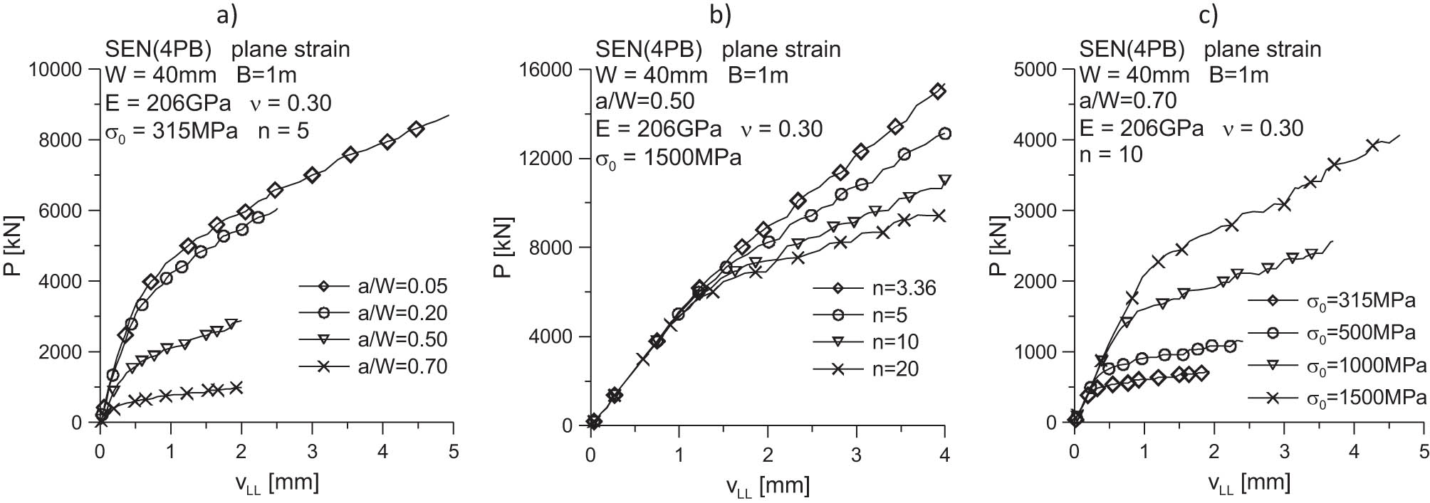
Influence of the relative crack length a/W (a), the strain hardening exponent n (b), and the yield point σ ₀ (c) on the P = f(v _LL) curves, used to determine energy A in formula (2).

The mutual arrangement of the P = f(v _LL) curves will not be commented on in this article – drawing obvious conclusions is left to the reader – the obtained arrangement of the P = f(v _LL)curves is as expected. It should be noted that only in terms of absolute values, the highest values of the force at the same level of load line displacement are observed for the SEN(4PB) specimens with the shortest cracks (Figure 13b) and for specimens characterized by the material with the highest yield point (Figure 14c). However, if in the graphs shown in Figure 13, on the ordinate axis, we replace the force (given in absolute values) with a relative value – the value of the force P is normalized by the limit load P ₀ (which, as we know, is different for each specimens – it depends linearly from the yield point and strongly on the crack length), the nature of the P/P ₀ = f(v _LL) curves will be completely different, as shown in Figure 14. A similar analysis – however, for typical and compliant with standards [1,2,3] SEN(B) specimens, was presented in ref. [13].

Figure 14

Influence of the relative crack length a/W (a), the strain hardening exponent n (b), and the yield point σ ₀ (c) on the P/P ₀ = f(v _LL) curves for SEN(4PB) specimens.

The inverted nature of the P/P ₀ = f(v _LL) curves is visible during the analysis of Figure 14a, where the influence of the relative crack length a/W on the distribution of the P/P ₀ = f(v _LL) curves is illustrated, with appointed the yield point σ ₀ and the strain hardening exponent n. Analyzing this graph, it can be argued with the fact that a specimen with a relative crack length a/W = 0.05 is characterized by the highest limit load – the longer the crack, the lower the limit load P ₀. In Figure 14b, there is no reversal of the trend in the arrangement of the P/P ₀ = f(v _LL) curves (with reference to the diagram presented in Figure 13b) the strain hardening exponent does not affect the limit load P ₀. Conversely, in Figure 14c, one can again observe a reversal of the tendency of the P/P ₀ = f(v _LL) curves, which is due to the fact that the limit load strongly depends on the yield point – the higher the yield point of the material, the greater the limit load level.

By transforming formula (2), it can be written that the η coefficient, numerically determined for energy A calculated from the area under the P = f(v _LL) curve, is equal to

(20) η = J ⋅ b ⋅ B A .

Based on formula (20), the values of the η coefficient were estimated for all 64 analyzed cases, and the results of the analysis were graphically presented in the form of graphs of changes in the η coefficient as a function of the J integral normalized by the product of the length of the noncracked specimen section b and the yield stress σ ₀ (Figure 15). The graphs present the changes in the η = f(J/(b·σ ₀)) curves and were prepared for three combinations to determine the influence of the relative crack length a/W (Figure 15a), the strain hardening exponent n in the R–O law (Figure 15b), and the yield point σ ₀ (Figure 15c). As can be seen, the value of the η coefficient initially increases slightly with the increasing external load, and then, depending on the geometric and material configuration of the SEN(4PB) specimen, it tends to reach the saturation level or slightly decreases. It is noticeable that in the case of SEN(4PB) specimens bent with pure moment, in contrast to the SEN(B) specimens discussed in ref. [13], the value of the η coefficient strongly depends on the relative crack length a/W (Figure 15a), slightly from the strain hardening exponent n in the R–O law (Figure 15b), and is also insensitive to the change in the value of the yield stress σ ₀ (Figure 15c). The value of the η coefficient clearly increases with the increase of the crack length a/W and very slightly with the decrease of the material hardening degree, expressed by the strain hardening exponent n in the R–O law. The value of the yield strength σ ₀ does not affect the value of the η factor. These properties will be used in the next steps of the analysis of the obtained set of numerical results.

Figure 15

Influence of the relative crack length a/W (a), the strain hardening exponent n (b), and the yield point σ ₀ (c) on the change of the η coefficient for SEN(4PB) specimens as a function of the increasing external load, expressed by J integral, normalized by the product of the length noncracked section of the specimen and the yield point – the η = f(J/(b·σ ₀)) curves.

Due to the complex nature of the changes in the η = f(J/(b·σ ₀)) curves, it is not possible to mathematically describe the changes in the η coefficient as a function of the integral J normalized by the product of the yield point and the physical length of the noncracked section of the specimen (J/(b·σ ₀)). Hence, to simplify the analysis and provide a concise formula allowing to estimate the value of the η coefficient depending on the material characteristics and geometry of the specimen (expressed in this article by the relative crack length a/W), the analysis scheme shown in refs [37,38] was used, which was also used in ref. [13]. Let us normalize equation (2) by dividing it on both sides by the product of the noncracked section of the specimen b and the yield stress σ ₀. Such a procedure leads to the following dependence:

(21) J b ⋅ σ 0 = η ⋅ A b 2 ⋅ σ 0 ⋅ B .

Denoted by:

(22) J ¯ = J b ⋅ σ 0 ,

(23) A ¯ = A b 2 ⋅ σ 0 ⋅ B .

The expression of the form is obtained

(24) J ¯ = η ⋅ A ¯ ,

which, after conversion, allows to write down the formula for the coefficient η:

(25) η = J ¯ A ¯ .

By plotting the changes of the normalized J integral denoted by J ¯ , as a function of the normalized energy A, denoted by A ¯ (Figure 16), and then analyzing them, we can confidently say that the value of the η coefficient is equal to the tangent of the φ angel (the slope of the J ¯ = f ( A ¯ ) curve to the abscissae). The analysis of Figure 7 leads to the same conclusions as in the case of the evaluation of the runs presented in Figure 15. The η coefficient depends on the relative crack length (a/W) and the strain hardening exponent (n). The value of the η coefficient is insensitive to the change in the yield stress of the material (σ ₀). These relationships were used in the next stage of analysis to propose the simple formula to calculate the η coefficient depending on the relative crack length and the strain hardening exponent. Table 8 presents all numerical results obtained during analysis.

$Figure 16 The influence of the relative crack length a/W (a), strain hardening exponent n (b), and yield stress σ 0 (c) on the estimated J ¯ = f ( A ¯ ) \bar{J}=f(\bar{A}) trajectories for SEN(4PB) specimens (based on ref. [13]). The η coefficient is equal to the tangent of the angel φ (the slope of the curve J ¯ = f ( A ¯ ) \bar{J}=f(\bar{A}) to the abscissae).$

Figure 16

The influence of the relative crack length a/W (a), strain hardening exponent n (b), and yield stress σ ₀ (c) on the estimated J ¯ = f ( A ¯ ) trajectories for SEN(4PB) specimens (based on ref. [13]). The η coefficient is equal to the tangent of the angel φ (the slope of the curve J ¯ = f ( A ¯ ) to the abscissae).

Table 8

The values of the η coefficients estimated based on numerical calculation and analytical analysis using equations (2) and (21–25)

n	σ ₀ (MPa)	a/W = 0.05	a/W = 0.20	a/W = 0.50	a/W = 0.70
n	σ ₀ (MPa)	η	η	η	η
3.36	315	0.25391	1.21755	3.18084	3.76528
5		0.28095	1.30231	3.27000	3.78768
10		0.41298	1.65036	3.33556	3.81304
20		0.55532	1.85169	3.37323	3.82626
3.36	500	0.24094	1.08699	3.11022	3.75878
5		0.31585	1.30345	3.19203	3.79852
10		0.43666	1.60267	3.28718	3.82981
20		0.55630	1.75512	3.29946	3.84156
3.36	1,000	0.26294	1.06342	3.02667	3.70433
5		0.30426	1.16961	3.10963	3.75112
10		0.41150	1.51666	3.17512	3.80855
20		0.55996	1.63483	3.18233	3.84106
3.36	1,500	0.27267	1.04368	3.00607	3.66916
5		0.27233	1.11500	3.06176	3.70757
10		0.39869	1.50130	3.12036	3.78234
20		0.54345	1.61274	3.15683	3.81267

The value of the η coefficient does not depend on the yield point (slight changes in the value of the η coefficient, up to 5%, are observed for the extreme analyzed yield points σ ₀ = 315 MPa and σ ₀ = 1,500 MPa). As the crack length increases, the value of the η coefficient increases significantly. Conversely, a variable influence of the strain hardening exponent on the value of the η coefficient is observed. For n = 3.36 and n = 20 and in the case of very short cracks (a/W = 0.05), the value of the η coefficient differs by almost 100%. In the case of short cracks (a/W = 0.20), the difference is a maximum of 40%, and in the case of normative and very long cracks (a/W = 0.50 and a/W = 0.70, respectively), the difference is less than 6%.

Figure 17a shows the total effect of the relative crack length a/W and the strain hardening exponent n in the R–O law on the value of the η coefficient, determined according to the diagram presented earlier (formulas (21–25)). As can be seen, the surface created on the basis of points determined by numerical calculations and analytical considerations proves the lack of dependence of the value of the η coefficient on the yield point and indicates a significant influence of the relative crack length and a weak influence of the strain hardening exponent in the R–O law. Therefore, using the Table Curve 3D package [33], an equation approximating the surface built on the basis of 64 research points was adjusted, which takes the following form:

(26) η = A 1 + A 2 n + A 3 ⋅ a W + A 4 n 2 + A 5 ⋅ a W 2 + A 6 n ⋅ a W + A 7 n 3 + A 8 ⋅ a W 3 + A 9 n ⋅ a W 2 + A 10 n 2 ⋅ a W ,

where A ₁–A ₁₀ denote the coefficients of matching formula (26) to points on the η = f(n, a/W) surface presented in Figure 17a. The coefficient of determination R ² for the presented figure is almost R ² = 0.997, and the matching coefficients are presented in Table 9.

$Figure 17 (a) Area η = f(n, a/W) – a summary of the values of the η coefficient obtained on the basis of numerical calculations and analytical considerations, as a function of the strain hardening exponent n in the R–O law and the relative fracture length a/W; (b) percentage values of residues – the difference between the values of the η coefficient determined on the basis of formula (26) and on the basis of the numerical and analytical procedure presented earlier on the basis of formulas (21 ÷ 25) and Figure 16 – the numerical and analytical results are presented in Figure 17a in the form of the η = f(n, a/W) surface (based on refs [13,37,38]).$

Figure 17

(a) Area η = f(n, a/W) – a summary of the values of the η coefficient obtained on the basis of numerical calculations and analytical considerations, as a function of the strain hardening exponent n in the R–O law and the relative fracture length a/W; (b) percentage values of residues – the difference between the values of the η coefficient determined on the basis of formula (26) and on the basis of the numerical and analytical procedure presented earlier on the basis of formulas (21 ÷ 25) and Figure 16 – the numerical and analytical results are presented in Figure 17a in the form of the η = f(n, a/W) surface (based on refs [13,37,38]).

Table 9

Coefficients of matching formula (26) to numerical results for SEN(4PB) specimens dominated by plane strain state

A ₁	A ₂	A ₃	A ₄	A ₅	A ₆	A ₇	A ₈	A ₉	A ₁₀	R ²
0.39263	−3.09406	6.88733	1.77465	1.22040	0.15084	10.74751	−5.98467	8.06867	−11.83204	0.99669

The analysis of Figure 17b shows that in selected cases, the approximation of all numerical results by the formula (26) is not the correct solution. For selected geometric and material configurations, too large differences are obtained between the values of the η coefficient determined on the basis of numerical calculations and analytical approach, and the values obtained on the basis of formula (26). Therefore, to minimize the differences in critical points, it is recommended to use formula (27) when looking for the desired values of the η coefficient, used separately for data described with the same yield point:

(27) η = A 1 + A 2 ⋅ n + A 3 ⋅ n 2 + A 4 ⋅ ln a W 1 + A 5 ⋅ n + A 6 ⋅ n 2 + A 7 ⋅ ln a W + A 8 ⋅ ln a W 2 ,

where the A ₁–A ₈ coefficients of approximation are presented in Table 10. The maximum difference in the case of using formula (27) and Table 10 is an error of about 7.5%.

Table 10

Coefficients of matching the formula (27) to the numerical results for SEN(4PB) specimens dominated by the plane strain state, for materials with different yield stress values σ ₀

σ ₀ (MPa)	315	500	1,000	1,500
A ₁	3.63346	3.75217	3.80032	3.71418
A ₂	0.23227	0.40461	0.27253	0.21887
A ₃	−0.00400	−0.00979	−0.00467	−0.00309
A ₄	0.98017	1.04201	0.87964	0.86285
A ₅	0.05069	0.09305	0.05238	0.03735
A ₆	−0.00066	−0.00205	−0.00044	0
A ₇	0.48687	0.45950	0.28053	0.26010
A ₈	0.70832	0.88539	0.84212	0.77915
R ²	0.999	0.999	0.999	0.998

4 Assessment of stress distribution in front of the crack tip

Full analysis and evaluation of stress distributions near the crack tip should include the tested 64 cases of material and geometric configuration, along with an analysis of the specimen reaching the limit load and full plasticization, which for elastic–plastic materials will not coincide with the limit load calculated according to the recommended formulas due to material strengthening. Such statements should be prepared for the successive main components of the stress tensor, which determine the level of known geometric constraints (Q stress, mean stress σ _m, and triaxiality coefficient T _z). Due to too many results, this article presents the selected results obtained in the course of numerical calculations. In the future, the author of this article does not exclude the development of a library of numerical solutions in the form of a proprietary application that allows viewing the stress distributions in front of the crack tip depending on the material and geometric configuration, along with a change of position in relation to the crack tip.

For the purposes of this study, it was decided that the evaluation of stress distributions near the crack tip will be performed for selected geometric and material cases for the standardized external load P/P ₀ ≈ 1.0. The following subjects were assessed:

effective stresses σ _eff determined according to the Huber-Mises-Hencky hypothesis, normalized by the yield point σ ₀ or by mean stresses σ _m, calculated as
(28) σ m = σ x x + σ y y + σ z z 3 ,
where the component σ _xx is the stress tensor component in the direction of the specimen thickness, and the components σ _yy and σ _zz are components in the crack propagation plane;
mean stresses σ _m normalized by the yield point σ ₀;
stress triaxiality factor T _z, defined by Guo [21–23], calculated as
(29) T z = σ x x σ y y + σ z z ,
principal components of the stress tensor – σ _yy, σ _zz, and σ _xx.

The parameters mentioned earlier (effective stresses, mean stresses, and stress triaxiality coefficient) are considered by many researchers to be measures of stress triaxiality and geometric constraints, influencing fracture toughness and fracture development in elastic–plastic materials.

Figures 18 and 19 show the influence of the relative crack length on the mentioned parameters and selected main components of the stress tensor. The graphs were prepared for both the physical distance from the crack tip and the normalized distance, calculated as r·J/σ ₀. The farther from the crack tip, the lower the value of the stress tensor components (Figure 19), and thus the effective stresses or mean stresses. Along with moving away from the crack tip, the value of the triaxiality stress coefficient T _z also decreases. As the crack length increases, the effective stresses and the stress triaxiality coefficient decrease are observed (Figure 18), with a simultaneous increase in the values of the main components of the stress tensor (Figure 19) – the shorter the crack, the lower the value of the successive components of the stress tensor – it is visible at the analysis of graphs presented as a function of the normalized distance from the fracture tip. The same behavior is observed for the analysis of changes in the mean stress values σ _m, also presented as a function of the normalized distance from the crack tip. It should also be noted that with the distance from the crack tip, in the tested measuring range, the value of the ratio of effective stresses and mean stresses increases – σ _eff/σ _m, while the increase in the crack length is accompanied by a decrease in its value (Figure 18a and b).

Figure 18

Influence of the relative crack length a/W on the distribution of selected parameters: σ _eff/σ ₀ and σ _eff/σ _m (a and b); σ _m/σ ₀ and T _z (c and d); T _z parameter (e and f), near the crack tip (graphs (a, c, and e) were prepared for the physical distance from the crack tip; graphs (b, d, and f) were prepared for the normalized distance from the crack tip ψ = r·J/σ ₀; the charts are presented for the moment when the external load reaches the limit load value – P/P ₀ = 1.00; with the following values of the J integral for subsequent specimens: a/W = 0.05, J = 31.0 kN/m; a/W = 0.20, J = 49.3 kN/m; a/W = 0.50, J = 29.3 kN/m; a/W = 0.70, J = 18.4 kN/m).

Figure 19

The influence of the relative crack length a/W on the distribution of the main stress tensor components: components in the plane of crack propagation σ _yy/σ ₀ (a and b) and σ _zz/σ ₀ (c and d) and the component in the thickness direction (along the crack front) σ _xx/σ ₀ (e and f) in front of the crack tip (graphs (a, c, and e) were prepared for the physical distance from the crack tip; graphs (b, d, f) were prepared for the normalized distance from the crack tip ψ = r·J/σ ₀; the charts are presented for the moment when the external load reaches the limit load value – P/P ₀ = 1.00; with the following values of the J integral for subsequent specimens: a/W = 0.05, J = 31.0 kN/m; a/W = 0.20, J = 49.3 kN/m; a/W = 0.50, J = 29.3 kN/m; a/W = 0.70, J = 18.4 kN/m.

Figures 20 and 21 show the effect of the hardening level on the stress distribution near the crack tip for SEN(4PB) specimens. The stronger the material strengthens (smaller value of the strain hardening exponent n in R–O law), the higher the stress tensor components are (Figure 21), similar to the effective stresses and average stresses normalized by the yield point (Figure 20). However, as shown in Figure 20e and f, along with a decrease in strengthening, an increase in the value of the stress triaxiality coefficient T _z is observed and an increase in the value of the ratio of effective stresses and mean stresses – σ_eff/σ _m, which in many scientific papers is considered a natural measure of geometric constraints in fracture mechanics. The less the material strengthens, the greater the value of the quotient σ _eff/σ _m, as in the case of the triaxiality coefficient T _z (Figure 20a and b).

Figure 20

Influence of the strain hardening exponent n on the distribution of parameters: σ _eff/σ ₀ and σ _eff/σ _m (a and b); σ _m/σ ₀ and T _z (c and d); T _z parameter (e and f), near the crack tip (graphs (a, c, and e) were prepared for the physical distance from the crack tip; graphs (b, d, and f) were prepared for the normalized distance from the crack tip ψ = r·J/σ ₀; the charts are presented for the moment when the external load reaches the limit load value – P/P ₀ = 1.00; with the following values of the J integral for subsequent specimens: n = 3.36, J = 547.4 kN/m; n = 5, J = 573.8 kN/m; n = 10, J = 651.1 kN/m; n = 20, J = 674.1 kN/m).

Figure 21

Influence of the strain hardening exponent n on the distribution of the main stress tensor components: components in the plane of crack propagation σ _yy/σ ₀ (a and b) and σ _zz/σ ₀ (c and d) and the component in the thickness direction (along the crack front) σ _xx/σ ₀ (e and f), near the crack tip (graphs (a, c, and e) were prepared for the physical distance from the crack tip; graphs (b, d, and f) were prepared for the normalized distance from the crack tip ψ = r·J/σ ₀; the charts are presented for the moment when the external load reaches the limit load value – P/P ₀ = 1.00; with the following values of the J integral for subsequent specimens: n = 3.36, J = 547.4 kN/m; n = 5, J = 573.8 kN/m; n = 10, J = 651.1 kN/m; n = 20, J = 674.1 kN/m).

Conversely, Figures 22 and 23 show the influence of the yield stress on selected parameters considered to be measures of geometrical constraints in the fracture mechanics (Figure 22) and on the main components of the stress tensor (Figure 23). In the case of the main components of the stress tensor, the influence of the yield stress is insignificant when the stress distributions are considered as a function of the physical distance from the crack tip (Figure 23(a, c, and e)). However, the change of the physical distance into its normalized form, denoted by ψ = r·J/σ ₀, indicates that with the increase in the yield point, the value of the successive components of the stress tensor decreases (Figure 23(b, d, and f)). In general, the fastest changes are observed for the component opening the fracture surfaces, denoted by σ _zz (Figure 23d). Also in the case of graphs presenting selected measures of geometric constraints (Figure 22(a and c)), a slight influence of the yield stress on the value of these parameters is observed (we are talking about the quotients σ _eff/σ ₀, σ _eff/σ _m, σ _m/σ ₀, and the T _z parameter), as long as they are considered as a function of the physical distance from the crack tip, denoted by r.

Figure 22

Influence of the yield point σ ₀ on the distribution of parameters: σ _eff/σ ₀ and σ _eff/σ _m (a and b); σ _m/σ ₀ and T _z (c and d); T _z parameter (e and f), near the crack tip (graphs (a, c, and e) were prepared for the physical distance from the crack tip; graphs (b, d, and f) were prepared for the normalized distance from the crack tip ψ = r·J/σ ₀; the charts are presented for the moment when the external load reaches the limit load value – P/P ₀ = 1.00; with the following J integral values for subsequent specimens: σ ₀ = 315 MPa, J = 15.6 kN/m; σ ₀ = 500 MPa, J = 34.3 kN/m; σ ₀ = 1,000 MPa, J = 175.3 kN/m; σ ₀ = 1,500 MPa, J = 336.2 kN/m).

Figure 23

Influence of the yield point σ ₀ on the distribution of the main stress tensor components: components in the plane of crack propagation σ _yy/σ ₀ (a and b) and σ _zz/σ ₀ (c and d) and the component in the thickness direction (along the crack front) σ _xx/σ ₀ (e and f), near the crack tip (graphs (a, c, and e) were prepared for the physical distance from the crack tip; graphs (b, d, and f) were prepared for the normalized distance from the crack tip ψ = r·J/σ ₀; the charts are presented for the moment when the external load reaches the limit load value – P/P ₀ = 1.00; with the following J integral values for subsequent specimens: σ ₀ = 315 MPa, J = 15.6 kN/m; σ ₀ = 500 MPa, J = 34.3 kN/m; σ ₀ = 1,000 MPa, J = 175.3 kN/m; σ ₀ = 1,500 MPa, J = 336.2 kN/m).

Conversely, when considering the distributions of the quotients σ _eff/σ ₀, σ _eff/σ _m, σ _m/σ ₀, and the T _z parameter as a function of the normalized position in front of the crack tip (Figure 22(b, d, and f)), it should be noted that the yield stress has a significant influence on the value of mean stress (Figure 22d) and the T _z parameter (Figure 22f). The greater the yield point, the lower the value of the mean stresses σ _m/σ ₀ and the T _z parameter. The value of effective stresses normalized by the yield point also slightly decreases (Figure 22b), and when normalizing the effective stresses by mean stresses, it can be noticed that the value of the quotient σ _eff/σ _m increases slightly with the increase of the yield stress of the material.

The conclusions and observations presented in this section are generally reflected in the other cases that were considered during the preparation of this article. In the future, the author intends to extend the scope of the research work with the analysis conducted for cases of three-dimensional beams subjected to bending in the fracture plane with a pure bending moment.

5 The Q stresses as a measure of in-plane geometric constraints

The Q stresses in the form known and used today were defined by O’Dowd and Shih in the early nineties of the last century [24,25]. It was one of the attempts to improve the description of the stress fields in front of the crack tip in elastic–plastic materials – so that the theoretical distribution differed as little as possible from the real one and would introduce new elements to the fracture mechanics. It turned out that the introduction of a two-parameter description (enrichment of the HRR solution by taking into account the influence of in-plane constraints) improves the result; however, the notion of a plane strain state or a plane stress state is still used. The idea of O’Dowd and Shih turned out to be a simple approach that was used in solving engineering problems in the form of inclusion in European programs SINTAP [SINTAP, 1999] and FITNET [FITNET, 2006]. In a series of papers [24,25,41], the authors concluded that the results obtained with the FEM are accurate and compared the differences between it and the HRR field. They proposed a description of the stress field in the form of the formula:

(30) σ i j σ 0 = J α ε 0 σ 0 I n r 1 / ( n + 1 ) ⋅ σ ˜ i j ( θ , n ) + Q r J / σ 0 q ⋅ σ ˆ i j ( θ , n ) ,

where the first part of the equation is the HRR solution [19,20], and the second part takes into account the influence of all other terms of the asymptotic expansion. In equation (30), J is the J integral, σ ₀ is the yield strength, ε ₀ is the strain in the uniaxial tensile direction corresponding to the yield stress (ε ₀ = σ ₀/E, where E is the Young’s modulus), n and α are material constants from the Ramberg-Osgoog relationship, I _n is a quantity dependent on the material through the strain hardening exponent n and the method of loading and thickness of the specimen, σ ˜ i j ( θ , n ) and σ ˆ i j ( θ , n ) are functions of the θ angle and the material constant n, which is similar to I _n function determined numerically, q is the exponent of the second term of the asymptotic expansion, and Q results from the fitting of equation (30) to the numerical solution obtained using the finite element method (FEM).

Conducting a series of studies, O’Dowd and Shih proposed the following equation to describe the stress field in front of the fracture front in elastic–plastic materials:

(31) σ i j = ( σ i j ) HRR + Q ⋅ σ 0 ⋅ σ ˆ i j ( θ ) ,

which significantly simplifies the description of the stress fields in front of the crack tip in elastic–plastic materials. The undoubted advantages of the solution represented by formula (31) over many descriptions of mechanical fields using a multiterm expansion are its simple form and easy way to obtain the value of the Q parameter, which is often referred to in the literature as “Q stress.” It should be remembered that in this case the Q stresses are not the second element of the asymptotic expansion, but the quantity taking into account influence the stress distribution of all terms of the higher-order expansion.

To avoid ambiguity in determining the value of the Q parameter, the authors in refs [24,25] determined that the most appropriate place to measure the Q stresses would be a point located at the distance r = 2.0·J/σ ₀ in the direction of θ = 0. The choice of the direction in which the Q parameter value is measured is not accidental, but dictated primarily by practical reasons. O’Dowd and Shih [24,25] postulated that the function σ ˆ i j ( θ ) on the direction θ = 0 should be equal to one. Thanks to this, the value of the Q parameter can be determined from the equation of the form:

(32) Q = ( σ θ θ ) FEM − ( σ θ θ ) HRR σ 0 for θ = 0 , and r ⋅ σ 0 J = 2 ,

where (σ _θθ)_FEM is the stress value determined numerically using FEM and (σ _θθ)_HRR is the stress value resulting from the HRR solution.

The Q parameter also referred to in the literature as Q stress has many characteristics. In the case of the dominance of the plane stress state, the values of Q stresses are close to zero, while for the case of the plane strain state, the Q parameter assumes negative values [8,34,35,42,43]. Its value for the plane strain case domination depends on

geometry of a construction element (specimen) – type of a structural element;
dimensions of a structural element – width and length of the crack;
material – yield point, strain hardening exponent;
method of loading – tension, bending;
the level of external load, expressed, for example, by the J integral (crack driving force) or by means of a real external load, normalized by a limit load.

The Q parameter is quite commonly used in problems in the field of fracture mechanics. It is used not only to describe stress fields but also to assess the strength of structural elements containing defects using failure assessment diagram (FAD) diagrams to lower the level of conservatism [7]. The Q parameter is also used in determining the actual fracture toughness, if the appropriate fracture criteria are used for this purpose [33].

That is why it is necessary to know the Q stresses – as a parameter correcting the stress field in front of the crack tip, as well as a parameter used in determining the actual fracture toughness. As a part of this study, the Q stress values were estimated for the considered beams with a crack subjected to four-point bending. This value was determined in the normalized distance (r·σ ₀)/J = 2, for the direction θ = 0, according to formula (32). The full results are 128 curves presenting the distribution of changes in the Q stress value as a function of the J integral (which is considered as the crack driving force) and the distribution of changes the Q stress as a normalized function the abscissa coordinate, written as log(J/(a·σ ₀)). Figures 24–26 present the selected results of the numerical analysis in a graphic form.

Figure 24

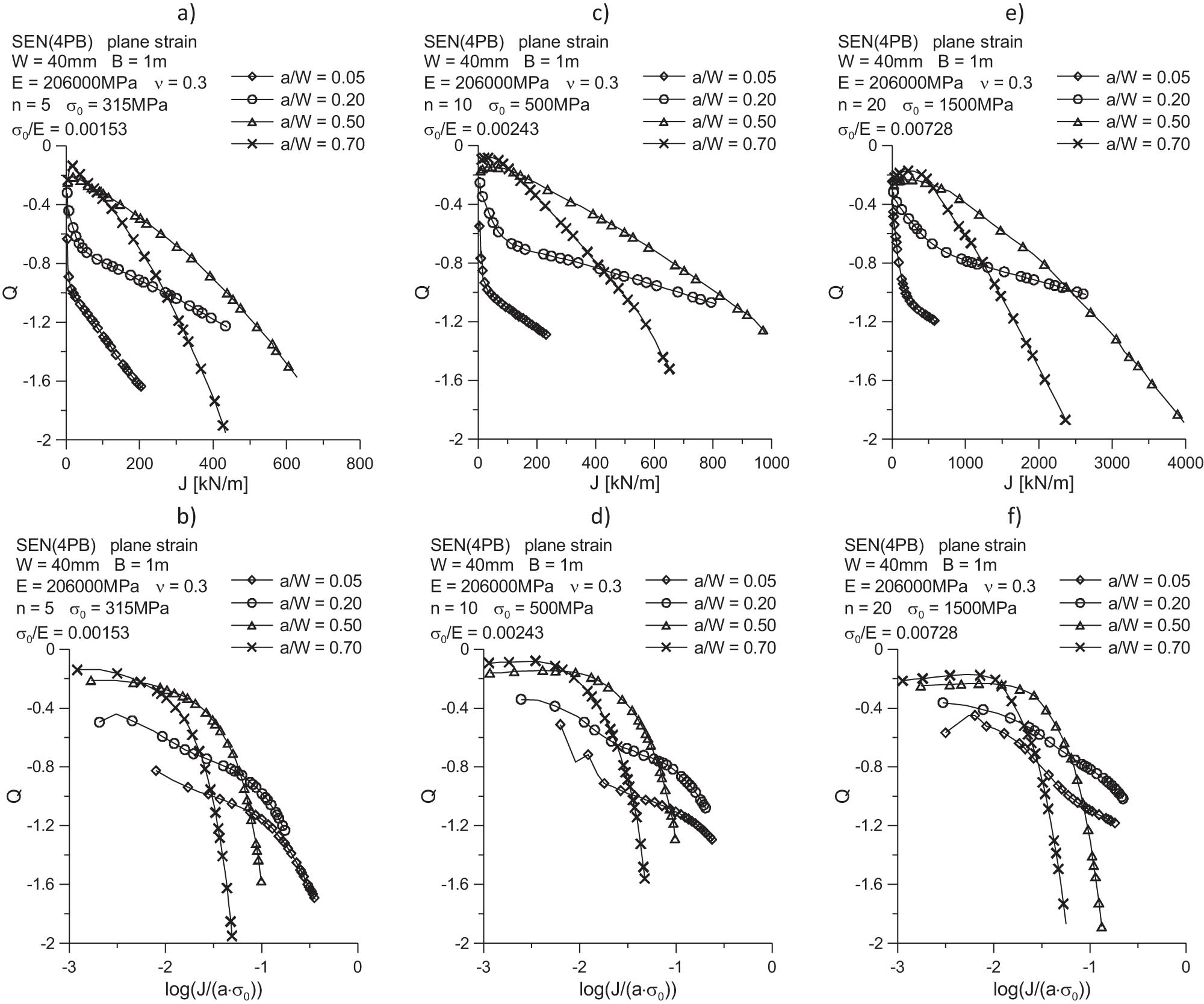
Influence of the relative crack length a/W on the distribution of the Q = f(J) and Q = f(log(J/(a·σ ₀))) curves for SEN(4PB) specimen dominated by the plane strain state: (a and b) n = 5, σ ₀ = 315 MPa; (c and d) n = 10, σ ₀ = 500 MPa; (e and f) n = 20, σ ₀ = 1,500 MPa.

Figure 25

Influence of the strain hardening exponent n on the distribution of the Q = f(J) and Q = f(log(J/(a·σ ₀))) curves for SEN(4PB) specimens dominated by the plane strain state: (a and b) σ ₀ = 315 MPa, a/W = 0.05; (c and d) σ ₀ = 500 MPa, a/W = 0.50; (e and f) σ ₀ = 1,500 MPa, a/W = 0.70.

Figure 26

Influence of the yield point σ ₀ on the distribution of the Q = f(J) and Q = f(log(J/(a·σ ₀))) curves for SEN(4PB) specimens dominated by the plane strain state: (a and b) n = 3.36, a/W = 0.05; (c and d) n = 10, a/W = 0.20; (e and f) n = 20, a/W = 0.50.

As can be seen, as the external load expressed by the J integral increases, the Q stress value decreases, assuming more and more negative values (Figures 24–26). The shorter the crack, the faster the changes in the Q stress value. When assessing the effect of the crack length, the behavior of the Q = f(J) and Q = f(log(J/(a·σ ₀))) curves cannot be considered as fixed – character of these changes is different for specimens with short cracks (a/W = 0.05 and a/W = 0.20) and long cracks (a/W = 0.50, a/W = 0.70). The analysis of the impact of the crack length on the distribution of the Q = f(J) and Q = f(log(J/(a·σ ₀))) curves is left to the reader based on Figure 24. It should be noted that the presented nature of the changes is generally consistent with the results obtained for other geometries with a predominance of bending, which the author mentioned in refs [8,35].

The analysis carried out in this article shows the unambiguous influence of the strain hardening exponent n (Figure 25). As can be seen, the stronger the material strengthens, the lower the Q stress value for the same J integral level (Figure 25). The increase in the crack length is accompanied by faster changes in the Q = f(log(J/(a·σ ₀))) curves – see Figure 25c and e. Depending on the geometric and material configuration, the difference between the Q stress values for two extreme materials with different levels of hardening (n = 3.36 and n = 20), with the same J integral level, may be greater than 0.8.

The established dependence and the established influence on the distribution of the Q = f(J) and Q = f(log(J/(a·σ ₀))) curves are also observed when assessing the dependence of these curves on the yield point (Figure 26). The higher the yield point, the higher the curves Q = f(J) and Q = f(log(J/(a·σ ₀))) lie, and the Q stresses at the same level of the J integral assume higher values. As can be seen, the pattern of the Q = f(J) and Q = f(log(J/(a·σ ₀))) curves changes with the increase of the crack length (Figures 25 and 26). The analysis of this fact, as in the case of Figure 24, is left to the reader. When assessing the value of Q stresses for two extreme yield stresses (σ ₀ = 315 MPa and σ ₀ = 1,500 MPa) considered in the course of numerical calculations, it can be noticed that at the same level of the J integral, the differences between them may be greater than 1.1. In the future, the author of this article intends to prepare a proprietary computer application that will allow viewing the collected results of numerical calculations in the graphic form and libraries in the form of PDF files.

Selected combinations of Q = f(log(J/(a·σ ₀))) curves presented in this article, along with other obtained results, were used to develop a catalog of numerical solutions, which were approximated by a third-degree polynomial. This approach allows to estimate the Q stress level without the need for tedious numerical calculations and quite complicated analyzes after their completion. The function selected to approximate the Q stresses is a function of the variable in the form of the parameter log(J/(a·σ ₀)):

(33) Q = A 1 + A 2 ⋅ log J a ⋅ σ 0 + A 3 ⋅ log J a ⋅ σ 0 2 + A 4 ⋅ log J a ⋅ σ 0 3 ,

where A ₁, A ₂, A ₃, and A ₄ are approximation factors, J is the J integral, a is the crack length, and σ ₀ is the yield point. It is recommended to enter physical quantities into the aforementioned formula after they have been converted to values corresponding to the basic units.

The use of formula (33) requires the user to know the current value of the J integral, the crack length a, the yield stress σ ₀, and the stain hardening exponent n in the R–O law. Formula (33) will correctly estimate the Q stresses in terms of material and geometric characteristics considered in this article. It should be remembered that the given values were obtained for a reference thickness of B = 1 m. The values of the approximation coefficients for the geometric and material configurations used in the research program, along with the coefficient of determination, are presented in Tables 11–14.

Table 11

Coefficients of matching formula (33) to the numerical results for the estimation of the Q stress values, for SEN(4PB) specimens dominated by the plane strain state, with the relative crack length a/W = 0.05

n	A ₁	A ₂	A ₃	A ₄	R ²	A ₁	A ₂	A ₃	A ₄	R ²
	a/W = 0.05, σ ₀ = 315 MPa, σ ₀/E = 0.00153					a/W = 0.05, σ ₀ = 500 MPa, σ ₀/E = 0.00243
3.36	−2.33382	−1.7292	−0.75811	−0.13926	0.988	−2.15619	−1.64319	−0.71819	−0.12869	0.993
5	−2.52935	−2.4184	−1.31664	−0.26262	0.994	−2.28605	−2.06325	−1.08162	−0.21575	0.989
10	−1.97818	−1.45456	−0.81505	−0.18303	0.992	−1.66775	−0.83436	−0.38719	−0.09979	0.979
20	−1.41572	−0.25872	−0.07296	−0.04333	0.991	−0.96781	0.666065	0.549307	0.077879	0.985

	a/W = 0.05, σ ₀ = 1,000 MPa, σ ₀/E = 0.00485					a/W = 0.05, σ ₀ = 1,500 MPa, σ ₀/E = 0.00728
3.36	−1.8884	−1.51936	−0.75848	−0.16004	0.997	−1.70931	−1.32262	−0.64414	−0.12977	0.995
5	−1.94578	−1.54344	−0.73781	−0.147	0.992	−1.79169	−1.31876	−0.58749	−0.11128	0.996
10	−1.49422	−0.4222	0.013601	0.001594	0.987	−1.60365	−0.7199	−0.14987	−0.02076	0.982
20	−0.84431	1.003735	0.892091	0.159418	0.996	−1.41354	−0.11871	0.279681	0.06309	0.979

Table 12

n	A ₁	A ₂	A ₃	A ₄	R ²	A ₁	A ₂	A ₃	A ₄	R ²
	a/W = 0.20, σ ₀ = 315 MPa, σ ₀/E = 0.00153					a/W = 0.20, σ ₀ = 500 MPa, σ ₀/E = 0.00243
3.36	−3.12706	−3.34302	−1.57043	−0.25947	0.997	−2.76319	−2.74765	−1.17439	−0.17502	0.995
5	−2.25695	−1.95005	−0.82109	−0.12932	0.991	−2.21099	−1.91192	−0.76224	−0.11128	0.990
10	−1.51217	−0.85899	−0.27151	−0.04161	0.988	−1.59032	−0.96878	−0.27504	−0.03352	0.987
20	−0.96415	−0.09001	0.093094	0.011457	0.988	−0.8585	0.196735	0.322012	0.061036	0.991

	a/W = 0.20, σ ₀ = 1,000 MPa, σ ₀/E = 0.00485					a/W = 0.20, σ ₀ = 1,500 MPa, σ ₀/E = 0.00728
3.36	−2.35984	−2.30144	−1.00243	−0.15365	0.997	−2.13123	−2.02452	−0.87872	−0.13381	0.998
5	−2.10291	−1.84559	−0.73288	−0.1057	0.995	−2.02815	−1.81203	−0.73865	−0.10708	0.997
10	−1.72941	−1.23923	−0.39369	−0.04673	0.991	−1.6862	−1.19601	−0.38337	−0.04561	0.998
20	−1.49005	−0.92013	−0.25977	−0.03153	0.986	−1.56695	−1.03826	−0.31925	−0.03967	0.996

Table 13

n	A ₁	A ₂	A ₃	A ₄	R ²	A ₁	A ₂	A ₃	A ₄	R ²
	a/W = 0.50, σ ₀ = 315 MPa, σ ₀/E = 0.00153					a/W = 0.50, σ ₀ = 500 MPa, σ ₀/E = 0.00243
3.36	−10.4003	−13.8555	−6.26863	−0.9305	0.987	−23.2066	−39.8359	−22.8925	−4.32185	0.978
5	7.983436	3.451663	0.481401	6.548557	0.998	−11.0695	−16.0994	−7.86404	−1.25473	0.978
10	−5.41782	−6.62589	−2.74558	−0.37469	0.992	−6.72414	−8.84597	−3.94117	−0.57997	0.996
20	−4.23841	−4.75998	−1.78852	−0.22076	0.998	−6.44854	−8.31086	−3.60263	−0.51676	0.994

	a/W = 0.50, σ ₀ = 1,000 MPa, σ ₀/E = 0.00485					a/W = 0.50, σ ₀ = 1,500 MPa, σ ₀/E = 0.00728
3.36	−15.9908	−24.6359	−12.4443	−2.01254	0.965	−12.3125	−18.6666	−9.53219	−1.58058	0.965
5	−11.3328	−16.6592	−8.15321	−1.28855	0.964	−10.7079	−16.0381	−8.09563	−1.32863	0.976
10	−8.47921	−11.7954	−5.49047	−0.83181	0.984	−9.3249	−13.6415	−6.72446	−1.08095	0.985
20	−8.78874	−12.2552	−5.67862	−0.85667	0.989	−8.78786	−12.4978	−5.97714	−0.93556	0.993

Table 14

n	A ₁	A ₂	A ₃	A ₄	R ²	A ₁	A ₂	A ₃	A ₄	R ²
	a/W = 0.70, σ ₀ = 315 MPa, σ ₀/E = 0.00153					a/W = 0.70, σ ₀ = 500 MPa, σ ₀/E = 0.00243
3.36	−32.4176	−42.7511	−18.7671	−2.71573	0.978	−34.6393	−45.8951	−20.0775	−2.87325	0.979
5	−20.688	−26.4432	−11.3463	−1.61406	0.992	−26.928	−35.2509	−15.2471	−2.16	0.968
10	−12.102	−14.2603	−5.67638	−0.7569	0.998	−13.335	−15.8783	−6.32245	−0.83436	0.993
20	−8.88792	−9.64743	−3.52043	−0.43134	1.000	−11.4469	−13.1089	−5.01322	−0.63741	0.995

	a/W = 0.70, σ ₀ = 1,000 MPa, σ ₀/E = 0.00485					a/W = 0.70, σ ₀ = 1,500 MPa, σ ₀/E = 0.00728
3.36	−28.3894	−37.2401	−16.1337	−2.27843	0.989	−22.742	−28.863	−12.2005	−1.69025	0.993
5	−28.7103	−38.3328	−16.8375	−2.40652	0.983	−23.795	−31.0052	−13.3534	−1.87815	0.991
10	−20.137	−25.8093	−10.9315	−1.51481	0.989	−23.7575	−31.6304	−13.9117	−1.99769	0.986
20	−17.3397	−21.6359	−8.94984	−1.21625	0.994	−19.1148	−24.4351	−10.3536	−1.43816	0.994

6 Summary

This article presents the results of analytical and numerical research focused on the determination of selected fracture mechanics parameters for beams containing a crack in the state of four-point bending with the dominance of a plane strain state. Based on a wide program of numerical calculations carried out for 16 hypothetical elastic–plastic materials differing in the yield point and the strain hardening exponent in the Ramberg–Osgood law, details of numerical modeling using the finite element method are presented. In the further part of this article, devoted to the obtained results of numerical calculations, the influence of geometry and material characteristics on numerically determined values of the J integral, crack tip opening displacement, and load line displacement would be discussed. For these values, new hybrid solutions were proposed, allowing to estimate them without the necessity to carry out tedious numerical calculations.

In the next stage, the mutual relationship between the J integral and the crack tip opening displacement was discussed, taking into account the influence of the in-plane constraints on the value of the d _n coefficient defined by the Shih relationship, giving appropriate approximation formulas. This article also verified the Landes and Begley formula, originally used to determine the J integral based on the graph of force versus the load line displacement, also taking into account the influence of the in-plane constraints on the value of the η coefficient, by making its value dependent on the yield point and relative crack length. Also in this part, the relevant numerical calculations were approximated, as presented earlier.

In addition to the assessment of the basic quantities in the field of fracture mechanics, this article presents a discussion on the stress distributions in front of the crack tip, as well as parameters commonly considered to be measurements of geometric constraints, among which a lot of attention was paid to the Q stresses defined by O’Dowd and Shih, with the impact of geometry and material characteristics on their values, as well as approximation formulas for 64 cases of geometric-material configuration, allowing to estimate their value without the need to carry out tedious numerical calculations.

The basic conclusions that can be drawn on the basis of the obtained results are as follows:

the lower the material hardening degree (higher value of the strain hardening exponent n in the R–O law), the higher the values of the elastic–plastic fracture mechanics parameters are obtained at the same level of external load;
the increase in the material strength (expressed as yield point σ ₀) is also accompanied by an increase in the value of the J integral, crack tip opening displacement δ _T, and load line displacement v _LL at the same level of external load;
the values of the functions h 1 ⁎ , h 2 ⁎ and h 3 ⁎ (which are needed to determine selected fracture parameters using new hybrid solutions) depend on the strain hardening exponent n, the relative crack length a/W, and the external load, but it is not possible for the aforementioned three functions define equal dependence on the specimen geometry or material characteristics;
the significant influence of the strengthening exponent on the level of the h ^* function is observed;
the yield point has the least influence on the change of the value of the h ^* function for the selected material and geometric characteristics;
the crack tip opening displacement is directly proportional to the J integral – the proportionality coefficient is the d _n coefficient, the value of which depends on yield stress, strain hardening exponent, and relative crack length;
the value of the η coefficient (which is needed to calculate the J integral values using the Landes and Begley formula) does not depend on the yield point;
as the crack length increases, the value of the η coefficient increases significantly and a variable influence of the strain hardening exponent on the value of the η coefficient is observed;
the farther from the crack tip, the lower the value of the stress tensor components, and thus, the effective stresses or mean stresses;
along with moving away from the crack tip, the value of the triaxiality stress coefficient T _z also decreases;
the stronger the material strengthens (smaller value of the strain hardening exponent n in R–O law), the higher the stress tensor components are, similarly to the effective stresses and average stresses normalized by the yield point;
in the case of the main components of the stress tensor, the influence of the yield stress is insignificant when the stress distributions are considered as a function of the physical distance from the crack tip;
the Q stress value depends on dimensions of a structural element (length of the crack), material (yield point, strain hardening exponent), and the level of external load, expressed by the J integral (which can be treated as crack driving force);
as the external load expressed by the J integral increases, the Q stress value decreases, assuming more and more negative values;
the shorter the crack, the faster the changes in the Q stress value;
the stronger the material strengthens, the lower the Q stress value for the same J integral level;
the increase in the crack length is accompanied by faster changes in the Q = f(log(J/(a·σ ₀))) curves;
the higher the yield point, the higher the curves Q = f(J) and Q = f(log(J/(a·σ ₀))) lie, and the Q stresses at the same level of the J integral assume higher values.

In the future, the author of this article intends to extend the analysis to three-dimensional cases and to consider issues related to the crack growth.

tel: +48-413424257

Funding information: This research was funded by the Director of the Discipline of Mechanical Engineering, at Faculty of Mechatronics and Mechanical Engineering at the Kielce University of Technology under the order number 01.0.09.00/1.02.001SUBB.MKTM.22.003.
Conflict of interest: Author states no conflict of interest.

References

[1] ASTM E. 1820-05 standard test method for measurement of fracture toughness. American Society for Testing and Materials; 2005.Search in Google Scholar

[2] PN-87/H-4335. Metals – Test method for fracture toughness for plane strain state domination; 1987 (Polish).Search in Google Scholar

[3] BS 7448. Fracture mechanics toughness tests. Method for determination KIC, critical CTOD and critical J values; 1991.Search in Google Scholar

[4] Kumar V, German MD, Shih CF. An engineering approach for elastic-plastic fracture analysis. EPRI Report NP-1931. Palo Alto, CA: Electric Power Research Institute; 1981.10.2172/6068291Search in Google Scholar

[5] SINTAP. Structural integrity assessment procedures for European industry. Final procedure, Brite-Euram Project No BE95-1426. Rotherham: British Steel; 1999.Search in Google Scholar

[6] API 579. Recommended practice for fitness-for-service. Washington, DC: American Petroleum Institute; 2000.Search in Google Scholar

[7] Kocak M, Webster S, Janosch JJ, Ainsworth RA, Koers R. FITNET report – European fitness-for-service network. Edited by contract no. G1RT-CT-2001-05071; 2006.Search in Google Scholar

[8] Graba M. The influence of material properties on the Q-stress value near the crack tip for elastic-plastic materials. J Theor Appl Mech. 2008;46(2):269–90.Search in Google Scholar

[9] Graba M. Catalogue of the numerical solutions for SEN(B) specimen assuming the large strain formulation and plane strain condition. Arch Civ Mech Eng. 2012;12(1):29–40.10.1016/j.acme.2012.03.005Search in Google Scholar

[10] Graba M. Proposal of the hybrid solution to determining the selected fracture parameters for SEN(B) specimens dominated by plane strain. Bull Pol Acad Sci Tech Sci. 2017;65(4):523–32.10.1515/bpasts-2017-0057Search in Google Scholar

[11] Nikishkov GP, Matvienko YG. Specimen thickness effect on elastic-plastic constraint parameter A. Frattura ed Integ Strutturale. 2015;33:73–9.10.3221/IGF-ESIS.33.10Search in Google Scholar

[12] Sulym H, Opanasovych V, Slobodian M, Bila O. Pure bending f strip (Beam) with crack in strip of tensile stress with allowance for plastic strips near crack tips. Acta Mech Auto. 2020;14(1):44–9.10.2478/ama-2020-0007Search in Google Scholar

[13] Delyavskyy M, Opanasovych V, Bilash O. Pure bending of a beam having crack perpendicular to its axis. AIP Conference Proceedings 2077; 2019. p. 020012.10.1063/1.5091873Search in Google Scholar

[14] Corbania S, Marthaa LF, de Castroa JT, Carterb B, Ingraffeab A. Crack front shapes and stress intensity factors in plates under a pure bending loading that induces partial closure of the crack faces. Proc Mater Sci. 2014;3:1279–84.10.1016/j.mspro.2014.06.207Search in Google Scholar

[15] Graba M. Determination of the limit load of a beam with a defect subjected to four-point bending – two-dimensional problems. Mechanik. 2016;4:282–7 (Polish).10.17814/mechanik.2016.4.37Search in Google Scholar

[16] Shih CF. Relationship between the J-integral and the crack opening displacement for stationary and extending cracks. J Mech Phys Solids. 1981;29:305–29.10.1016/0022-5096(81)90003-XSearch in Google Scholar

[17] Gałkiewicz J, Graba M. Algorithm for determination σij˜(n,θ), εij˜(n,θ), ui˜(n,θ), dn(n) and In(n) functions in hutchinson-rice-rosengren solution and its 3d generalization. J Theor Appl Mech. 2006;44(1):19–30.Search in Google Scholar

[18] Landes JD, Begley JA. Test results from J-integral studies: an attempt to establish a JIC testing procedure fracture analysis. ASTM STP 560. Philadelphia: American Society for Testing and Materials; 1974. p. 170–8610.1520/STP33140SSearch in Google Scholar

[19] Hutchinson JW. Singular behaviour at the end of a tensile crack in a hardening material. J Mech Phys Solids. 1968;16:13–31.10.1016/0022-5096(68)90014-8Search in Google Scholar

[20] Rice JR, Rosengren GF. Plane strain deformation near a crack tip in a power-law hardening material. J Mech Phys Solids. 1968;16:1–12.10.21236/AD0659300Search in Google Scholar

[21] Guo W. Elastoplastic three dimensional crack border field – I. Singular structure of the field. Eng Fract Mech. 1993;46(1):93–104.10.1016/0013-7944(93)90306-DSearch in Google Scholar

[22] Guo W. Elastoplastic three dimensional crack border field – II. Asymptotic solution for the field. Eng Fract Mech. 1993;46(1):105–13.10.1016/0013-7944(93)90307-ESearch in Google Scholar

[23] Guo W. Elastoplastic three dimensional crack border field – III. Fracture parameters. Eng Fract Mech. 1995;51(1):51–71.10.3901/JME.2015.09.051Search in Google Scholar

[24] O’Dowd NP, Shih CF. Family of crack-tip fields characterized by a triaxiality parameter – I. Structure of fields. J Mech Phys Solids. 1991;39(8):989–1015.10.1016/0022-5096(91)90049-TSearch in Google Scholar

[25] O’Dowd NP, Shih CF. Family of crack-tip fields characterized by a triaxiality parameter – II. Fracture applications. J Mech Phys Solids. 1992;40(5):939–63.10.1016/0022-5096(92)90057-9Search in Google Scholar

[26] ADINA. User interface command reference manual – Volume I: ADINA solids & structures model definition, report ARD 11-2. ADINA R&D, Inc.; 2011.Search in Google Scholar

[27] ADINA. Theory and modeling guide – Volume I: ADINA Solids & structures, report ARD 11-8. ADINA R&D, Inc.; 2011.Search in Google Scholar

[28] Brocks W, Cornec A, Scheider I. Computational aspects of nonlinear fracture mechanics, bruchmechanik. GKSS-Forschungszentrum, Geesthacht, Germany: Elsevier; 2003. p. 127–209.10.1016/B0-08-043749-4/03102-5Search in Google Scholar

[29] Brocks W, Scheider I. Reliable J-Values. Numerical Aspects of the Path-Dependence of the J-integral in Incremental Plasticity. Bruchmechanik. GKSS-Forschungszentrum, Geesthacht, Germany: Elsevier; 2003. p. 264–74.10.1515/mt-2003-450608Search in Google Scholar

[30] Graba M, Gałkiewicz J. Influence of the crack tip model on results of the finite element method. J Theor Appl Mech. 2007;45(2):225–37.Search in Google Scholar

[31] Sherry AH, Wilkes MA, Beardsmore DW, Lidbury DPG. Material constraint parameters for the assessment of shallow defects in structural componenets – Part I: Parameter solutions. Eng Fract Mech. 2005;72:2373–95.10.1016/j.engfracmech.2004.12.009Search in Google Scholar

[32] Sherry AH, Hooton DG, Beardsmore DW, Lidbury DPG. Material constraint parameters for the assessment of shallow defects in structural components – Part II: constraint – based assessment of shallow cracks. Eng Fract Mech. 2005;72:2396–415.10.1016/j.engfracmech.2004.12.010Search in Google Scholar

[33] Graba M. On the fracture criteria for elastic-plastic materials. Mechanik. 2017;12:1174–79 (Polish).10.17814/mechanik.2017.12.201Search in Google Scholar

[34] Graba M. Numerical analysis of the influence of in-plane constraints on the crack tip opening displacement for SEN(B) specimens under predominantly plane strain conditions. Int J Appl Mech Eng. 2016;21(4):849–66.10.1515/ijame-2016-0050Search in Google Scholar

[35] Graba M. The characteristics of selected triaxiality measures of the stresses for a C(T) specimen dominated by the plane strain state. Int J Appl Mech Eng. 2020;25(1):52–74.10.2478/ijame-2020-0005Search in Google Scholar

[36] Lindqvist S, Kuutti J. Dependence between η-factor and crack location relative to a fusion boundary between hard and soft materials in a SE(B) specimen. Int J Fract. 2018;211:281–93.10.1007/s10704-018-0288-5Search in Google Scholar

[37] Ruggieri C. Further results in J and CTOD estimation procedures for SE(T) fracture specimens – Part I: homogeneous materials. Eng Fract Mech. 2012;79:245–65.10.1016/j.engfracmech.2011.11.003Search in Google Scholar

[38] Barbosa VS, Ruggieri C. Fracture toughness testing using non-standard bend specimens – Part I: constraint effects and development of test procedure. Eng Fract Mech. 2018;195:279–96.10.1016/j.engfracmech.2018.03.029Search in Google Scholar

[39] Kawabata T, Tagawa T, Kayamori Y, Mikami Y, Kitano H, Tonan T, et al. Investigation on η and m factors for J integral in SE(B) specimens. Theor Appl Fract Mech. 2018;97:224–35.10.1016/j.tafmec.2018.08.013Search in Google Scholar

[40] Table Curve 3D Version 4.0 – manual instructions for users; 2002.Search in Google Scholar

[41] Shih CF, O’Dowd NP, Kirk MT. A framework for quantifying crack tip constraint. Constraint effects in fracture. ASTM STP 1171. Philadelphia: American Society for Testing and Materials; 1993. p. 2–20.10.1520/STP18020SSearch in Google Scholar

[42] Graba M. A numerical analysis of selected elastic-plastic fracture parameters for DEN(T) plates under plane strain conditions. Int J Appl Mech Eng. 2017;22(1):49–80.10.1515/ijame-2017-0004Search in Google Scholar

[43] Graba M. The influence of material properties and crack length on the Q-stress value near the crack tip for elastic-plastic materials for single edge notch plate in tension. Arch Civ Mech Eng. 2011;11(2):301–19.10.1016/S1644-9665(12)60145-9Search in Google Scholar

Received: 2021-10-10

Revised: 2021-12-14

Accepted: 2022-01-04

Published Online: 2022-03-04

This work is licensed under the Creative Commons Attribution 4.0 International License.

Articles in the same Issue

https://doi.org/10.1515/eng-2022-0008

Keywords for this article

J integral; crack tip opening displacement; load line displacement; limit load; constraints; stress distributions; Q stress; in-plane constraints

Creative Commons

BY 4.0

Constraint evaluation and effects on selected fracture parameters for single-edge notched beam under four-point bending

Article

Abstract

1 Introduction

2 Details of numerical calculations, specimen geometry, and material of the specimen

3 Characteristics of selected fracture mechanics parameters

3.1 Hybrid solutions for estimating the basic parameters of fracture mechanics

3.2 Shih relationship analysis – mutual relation of the crack tip opening displacement δ T and the J integral

3.3 Evaluation of the η coefficient in the Landes and Begley formula for the calculation of the J integral

4 Assessment of stress distribution in front of the crack tip

5 The Q stresses as a measure of in-plane geometric constraints

6 Summary

References

Articles in the same Issue

Articles in the same Issue

Articles in the same Issue

3.2 Shih relationship analysis – mutual relation of the crack tip opening displacement δ _T and the J integral