Intelligent temporal analysis of coronavirus statistical data

Esko K. Juuso

doi:10.1515/eng-2021-0118

Article Open Access

Intelligent temporal analysis of coronavirus statistical data

Esko K. Juuso

Published/Copyright: December 31, 2021

Published by

Become an author with De Gruyter Brill

Submit Manuscript Author Information

From the journal Open Engineering Volume 11 Issue 1

Abstract

The coronavirus COVID-19 is affecting around the world with strong differences between countries and regions. Extensive datasets are available for visual inspection and downloading. The material has limitations for phenomenological modeling but data-based methodologies can be used. This research focuses on the intelligent temporal analysis of datasets in developing compact solutions for early detection of levels, trends, episodes, and severity of situations. The methodology has been tested in the analysis of daily new confirmed COVID-19 cases and deaths in six countries. The datasets are studied per million people to get comparable indicators. Nonlinear scaling brings the data of different countries to the same scale, and the temporal analysis is based on the scaled values. The same approach can be used for any country or a group of people, e.g., hospital patients, patients in intensive care, or people in different age categories. During the pandemic, the scaling functions expanded for the confirmed cases but remained practically unchanged for the confirmed deaths, which is consistent with increasing testing.

Keywords: intelligent methods; temporal analysis; coronavirus; COVID-19

1 Introduction

The coronavirus COVID-19 is affecting around the world. There are strong differences between countries and regions. People of all ages can be infected, but older people and people with pre-existing medical conditions are more vulnerable to becoming severely ill. The risk is presented with three parameters:

Transmission rate evaluated by the number of newly infected people.
Case fatality rate (CFR) based on the percent of cases that result in death.
Vaccine performance as a prevention measure.

An online interactive dashboard is hosted by the Center for Systems Science and Engineering (CSSE) at Johns Hopkins University for visualizing and tracking reported cases of coronavirus disease 2019 (COVID-19) in real time [1,2]. Transmission dynamics is difficult to explain since the characteristics of a novel disease include many uncertainties. The open evidence review [3] makes information about active research on modes of transmission available.

The effective reproduction number (R) of an infectious disease is used for modeling. The tracking of the parameter is done by assuming a model structure. An example of this approach is presented in ref. [4], where the Kalman filter and a SIR model have been used for tracking R for COVID-19.

Distributions of the variables provide useful information about fluctuations, trends, and models. This has been used in temporal analysis for all types of measurements, features, and indices. Recursive updates of the parameters are needed in prognostics [5].

Generalized norms are used in data analysis to extract features from waveform signals collected from the statistical databases [6]. The computation of the norms can be divided into the computation of equal sized sub-blocks, i.e., the norm for several samples can be obtained as the norm for the norms of individual samples. This means that norms can be recursively updated [7]. The same methodologies can be used for analyzing the data distributions in less frequent data, e.g., daily COVID-19 data.

The temporal analysis focused on important variables provides useful information, including trends, fluctuations, and anomalies. The fundamental elements are presented geometrically as triangles to describe local temporal patterns originating from qualitative reasoning and simulation [8,9,10]. Replacing the reasoning with calculations based on the scaled values was the main contribution in ref. [11,12].

This research aims to develop unified intelligent temporal analysis methodologies for detecting the fluctuations, trends, and severity of the corona situations. Parametric systems are used to adapt the solution for varying operating conditions caused by local areas and groups of people. Recursive updates are used in the parametric models.

2 COVID-19 data

This research uses the complete COVID-19 dataset maintained by Our World in Data [13]. The collection of the COVID-19 data is updated daily and includes data on confirmed cases, deaths, hospitalizations, and testing. Raw data on confirmed cases and deaths for all countries are sourced from the COVID-19 Data Repository by the Center for Systems Science and Engineering (CSSE) at Johns Hopkins University. Data visualizations rely on work from many different people and organizations [14].

The Our World in Data has created a new description of all our data sources available at the GitHub repository where all of the data can be downloaded. These datasets were used as a data source in this research. The collection of data is presented as tabular data where every column of a table represents a particular variable, and each row corresponds to a given record of the data set for a specific country on a certain day. Each record consists of one or more fields, separated by commas. The data can be visualized in the COVID-19 DataExplorer for individual countries. Several countries can be compared by selecting them for the view. The maps available in DataExplorer help in focusing on the analysis.

The analysis uses confirmed COVID-19 cases whose number is lower than the number of actual cases. The main reason for this is limited testing, which also varies between countries and time. Therefore, the analysis is done country-wise. The pandemic introduces an increasing number of new COVID-19 cases, but countries also make progress in reducing the speed toward zero new cases (Figure 1). However, the increase can start again as can be seen in the data of different countries. The pandemic can restart if it is active somewhere. The difficult periods vary between countries.

Figure 1

Daily new confirmed COVID-19 cases per million people, rolling 7-day averages collected from [13] for selected countries.

A part of the pandemic cases leads to hospitalizations and deaths. Both increases and reductions can be seen in the daily new confirmed COVID-19 deaths (Figure 2). During the outbreak of the pandemic, the calculated case fatality rate (CFR) was a poor measure of the mortality risk since it depends on the number of tests, and at that time, there were few tests. The true number of cases was much higher. Later the number of tests has increased strongly, but not in all countries.

Figure 2

Daily new confirmed COVID-19 deaths per million people, rolling 7-day averages collected from ref. [13] for selected countries.

An increasing number of variants and mutations has effects on the number of cases. Vaccinations were just started during the studied period. All these have a strong effect on the dynamics of the pandemic. The problems become more case specific but can, in the same time, activate in many locations.

The research focused on the temporal analysis is aimed at finding situations for more detailed modeling and action planning.

3 Methodologies

The temporal analysis needs to be adapted in the appropriate situations. The unified temporal analysis requires that all the features are on the same scale. In this research, this is done by combining the nonlinear scaling and the intelligent temporal analysis. This methodology allows recursive updates of the scaling functions.

3.1 Nonlinear scaling

The nonlinear scaling brings various measurements and features to the same scale by using monotonously increasing scaling functions x j = f ( X j ) , where x j is the variable and X j is the corresponding scaled variable. The function f ( ) consists of two second-order polynomials, one for the negative values of X j and one for the positive values, respectively. The corresponding inverse functions X j = f − 1 ( x j ) based on square root functions are used for scaling to the range [ − 2 , 2 ], denoted as linguistification. The monotonous functions allow scaling back to the real values by using the function f ( ) [15].

The parameters of the functions are extracted from measurements by using generalized norms and moments. The support area is defined by the minimum and maximum values of the variable, i.e., a specific area for each variable j , j = 1 , … , m . The central tendency value, c j , divides the support area into two parts, and the core area is defined by the central tendency values of the lower and the upper part, ( c l ) j and ( c h ) j , correspondingly. This means that the core area of the variable j defined by [ ( c l ) j , ( c h ) j ] is within the support area.

The corner points are defined by iterating the orders, p , of the corresponding generalized norms:

(1) ‖ M j p τ ‖ p = ( M j p ) 1 / p = 1 N ∑ i = 1 N ( x j ) i p 1 / p ,

where p ≠ 0 is calculated from N values of a sample and τ is the sample time. This provides possibilities to recursively update the scaling functions since the generalized norms can be recursively updated. The iteration is based on the generalized skewness [16].

The scaled values should preserve the directions of the temporal changes with time. To achieve this, the scaling functions should be monotonously increasing. This is achieved by limiting the ratios,

(2) α j − = ( c l ) j − min ( x j ) c j − ( c l ) j , α j + = max ( x j ) − ( c h ) j ( c h ) j − c j ,

in the range 1 3 , 3 . The corner points are adjusted if these limitations are not filled. There are several alternatives to select the points to tune [17].

The second-order polynomials,

(3) f j − = a j − X j 2 + b j − X j + c j , X j ∈ [ − 2 , 0 ) , f j + = a j + X j 2 + b j + X j + c j , X j ∈ [ 0 , 2 ] ,

are monotonously increasing if the coefficients are defined as follows:

(4) a j − = 1 2 ( 1 − α j − ) Δ c j − , b j − = 1 2 ( 3 − α j − ) Δ c j − , a j + = 1 2 ( α j + − 1 ) Δ c j + , b j + = 1 2 ( 3 − α j + ) Δ c j + ,

where Δ c j − = c j − ( c l ) j and Δ c j + = ( c h ) j − c j .

3.2 Temporal analysis

Trend analysis produces useful indirect measurements for the early detection of changes. For any variable j , a trend index I j T ( k ) is calculated from the scaled values X j with a linguistic equation:

(5) I j T ( k ) = 1 n S + 1 ∑ i = k − n S k X j ( i ) − 1 n L + 1 ∑ i = k − n L k X j ( i ) ,

which is based on the means obtained for a short and a long time period, defined by delays n S and n L , respectively. The index value is in the linguistic range [ − 2 , 2 ] , representing the strength of both decrease and increase of the variable x j [11,12].

An increase is detected if the trend index exceeds a threshold I j T ( k ) > ε 1 + . Correspondingly, I j T ( k ) < − ε 1 − for a decrease. Trends are linear if the derivative is close to zero: − ε 2 − < Δ I j T ( k ) < − ε 2 + . The derivative of the index I j T ( k ) , denoted as Δ I j T ( k ) , is used for analyzing the full set of the triangular episodic representations (Figure 3), which cover different alternative risks related to high and low values.

$Figure 3 Triangular episodic representations defined by the index I j T ( k ) {I}_{j}^{T}\left(k) and the derivative Δ I j T ( k ) \Delta {I}_{j}^{T}\left(k) .$

Figure 3

Triangular episodic representations defined by the index I j T ( k ) and the derivative Δ I j T ( k ) .

In the analysis of the COVID data, the high number of cases is harmful. Area D close to [ 2 , 2 ] is a dangerous situation, which introduces warnings and alarms. The increase becomes slower in Area A , the unfavorable trend is stopping and turns to decrease in Area B close to [ − 2 , − 2 ] . The decrease gets slower in Area C and gradually stops.

The episodes are not sufficient for analyzing the severity of the situation. The level X j ( k ) , which is naturally highly important, is included in a deviation index, I j D ( k ) , which is a weighted sum of X j ( k ) , I j T ( k ) , and Δ I j T ( k ) . In this case, this index has its highest absolute values, when the level X j ( k ) is very high and getting still higher with a fast increasing speed [11]. This can be understood as a third dimension in Figure 3.

The trend analysis is tuned to applications by selecting the time periods n L and n S . Further fine-tuning can be done by adjusting the weight factors w j T 1 and w j T 2 used for the indices I j T ( k ) and Δ I j T ( k ) . The default thresholds ε 1 + = ε 1 − = ε 2 + = ε 2 − = 0.5 . The calculations are done with numerical values, and the results are understandable in natural language. The scaled values in the range [ − 2 , 2 ] can be represented with appropriate linguistic terms.

The fluctuation indicators calculate the difference of the high and the low values of the measurement as a difference of two moving generalized norms:

(6) Δ x j F ( k ) = ‖ K s τ M j p h ‖ p h − ‖ K s τ M j p l ‖ p l ,

where the orders p h ∈ ℜ and p l ∈ ℜ are large positive and negative, respectively. The moments are calculated from the latest K s + 1 values, and an average of several latest values of Δ x j F ( k ) is used as an indicator [18].

4 Data analysis

The analysis was done for daily new confirmed COVID-19 cases and deaths in six countries: Finland, India, Italy. Sweden, the United Kingdom, and the United States. The full dataset with all the countries was downloaded for a selected time period as a csv file by using the DataExplorer. The country-specific lines were then extracted from this file to the arrays. The rolling 7-day average was used for the feasibility study since it operated smoothly for the confirmed deaths as well.

The cases were analyzed per million people to improve the sensitivity of the analysis for small countries. The situations vary strongly between countries and periods of time. The normalization keeps the directions of the effects but would leave the analysis of nonlinear effects to the modeling. The nonlinear scaling approach aims to simplify the modeling work.

Within each country, the risk levels are represented by using nonlinear scaling. The scaling functions are defined by five corner points by generalized norms whose orders are obtained from the data. The real values are scaled to the same range [ − 2 , 2 ] for all variables in each country.

Trend indices are calculated from the scaled values by using informative short and long time periods. The trend index and its derivative visualize trend episodes. The severity of the situation is evaluated by a deviation index, which combines the trend index, the derivative of it, and the level.

The calculations are done with numerical values, and the results are represented in natural language.

5 Results

5.1 Confirmed cases

5.1.1 Scaling functions

Daily new confirmed COVID-19 cases are varying strongly (Figure 1). The parameters of the scaling function are analyzed separately for each country in the same way. The analysis iterates the orders of the generalized norms, which are the central tendency values of all the values (center), the lower part (left), and the upper part (right). For Finland, these orders are shown in Figure 4: p = 1.7852 for the value c j (center), p = 1.7617 for the point ( c l ) j (left), and p = 2.4844 for the point ( c h ) j (right) fill the condition γ 3 = 0 for the skewness. In the same time, these are the minimum points of the kurtosis γ 4 (Figure 4). All these orders are much higher than the arithmetic mean, actually fairly close to the standard deviation. The corresponding real values are shown in Figure 5. The support area is [ min x j , max x j ] by default.

Figure 4

Analysis of parameters for the new confirmed cases in Finland.

$Figure 5 Parameters min ( x j ) \min \left({x}_{j}) , ( c l ) j {\left({c}_{l})}_{j} . c j {c}_{j} , ( c h ) j {\left({c}_{h})}_{j} and max ( x j ) \max \left({x}_{j}) for the daily new confirmed cases: first 240 days (left) and all data (right).$

Figure 5

Parameters min ( x j ) , ( c l ) j . c j , ( c h ) j and max ( x j ) for the daily new confirmed cases: first 240 days (left) and all data (right).

The resulting scaling function is nonlinear and consists of two second-order polynomials with linear derivatives. The upper part is slightly steeper than the lower part (Figure 6). A continuous derivative in the center was not required in the calculations. The scaling functions were analyzed separately for the first seven months of the epidemic since the testing was on a much lower level. The feasible area expands considerably after the first periods. Obviously, the true number of cases was not detected earlier.

Figure 6

Nonlinear scaling for the new confirmed cases in Finland: scaling function (upper curve) and derivative (lower curve).

5.1.2 Temporal analysis

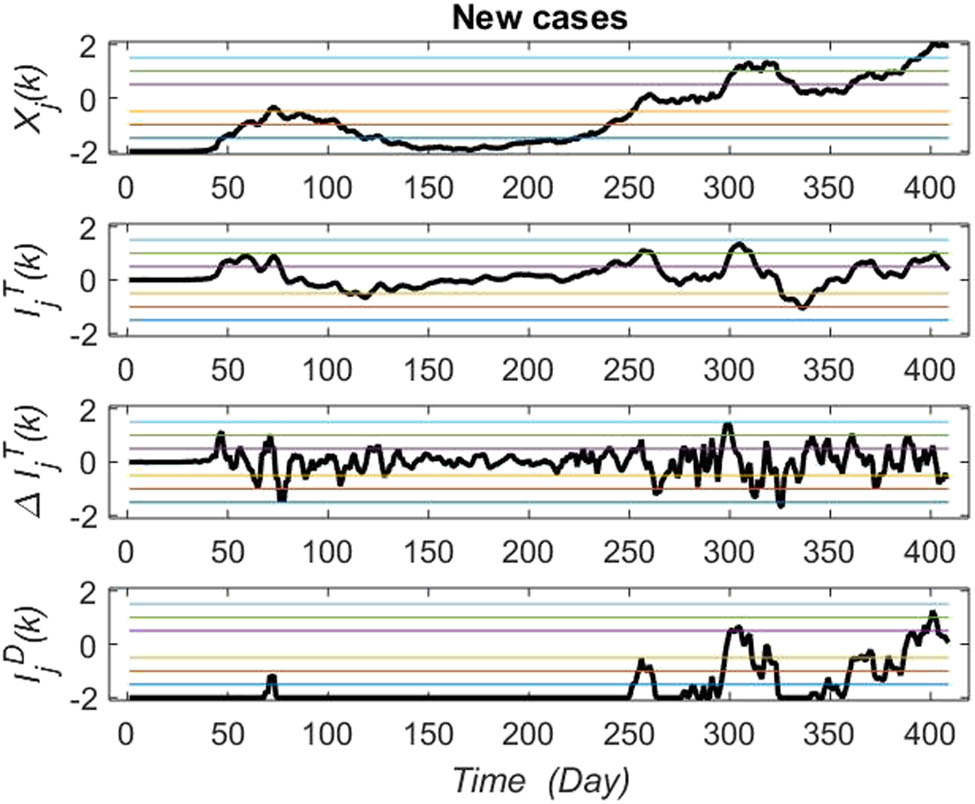
The scaled values X j for different countries are calculated by using appropriate scaling functions (3). The index I j T ( k ) and the derivative Δ I j T ( k ) represent the corresponding temporal effects and indicate the temporal episodes. The severity of the situation represented by I j D ( k ) combines all these. For Finland, the results calculated from the full data are shown in Figures 7 and 8.

Figure 7

Temporal analysis for the new confirmed cases in Finland.

Figure 8

Temporal episodes for the new confirmed cases in Finland.

The index I j T ( k ) and the derivative Δ I j T ( k ) are active all the time. Also, different trend episodes are detected efficiently (Figure 8). The deviation index I j D ( k ) is very low until Autumn since the values X j ( k ) are low. The need for the recursive tuning is clear during the autumn period. In the starting part until Day 240, the sensitivity of the analysis was improved by using only this part of the data for tuning the scaling functions. Then the index I j D ( k ) starts to react (Figure 9). Also, episodes are detected in a wider area.

Figure 9

Temporal analysis for the new confirmed cases during the starting part until Day 240 in Finland.

For the real-time operation, the analysis should adapt to the changing situations: the scaling functions should be gradually expanded in the beginning periods to react to increased testing and vaccinations and new variants. The orders p should be re-evaluated at least two times during the Autumn. The need for recursive updates may provide indications of the activation of new variants.

5.2 Confirmed deaths

5.2.1 Scaling functions

Daily new confirmed COVID-19 deaths are varying strongly (Figure 2). The analysis was performed for this data in the same way as for the confirmed cases. The corner points are shown in Figure 10. The differences between the beginning part and the whole data are very small. As an example, the analysis and the functions are shown for Finland in Figures 11 and 12. Nonlinear effects are even steeper than for the confirmed cases. For the upper part, the order is much higher: p = 3.7188 .

$Figure 10 Parameters min ( x j ) \min \left({x}_{j}) , ( c l ) j {\left({c}_{l})}_{j} . c j {c}_{j} , ( c h ) j {\left({c}_{h})}_{j} , and max ( x j ) \max \left({x}_{j}) for the daily new confirmed deaths: first 240 days (left) and all data (right).$

Figure 10

Parameters min ( x j ) , ( c l ) j . c j , ( c h ) j , and max ( x j ) for the daily new confirmed deaths: first 240 days (left) and all data (right).

Figure 11

Analysis of parameters for the new confirmed deaths in Finland.

Figure 12

Nonlinear scaling for the daily new confirmed deaths in Finland: scaling function (upper curve) and derivative (lower curve).

5.2.2 Temporal analysis

The temporal analysis for the confirmed deaths was done in the same way as for the confirmed cases: scaled values obtained with the appropriate scaling functions, then trend indices I j T ( k ) and derivatives Δ I j T ( k ) , and finally, the severity of situations with deviation indices. For Finland, the results calculated from the full data are shown in Figures 13 and 14.

Figure 13

Temporal analysis for the new confirmed deaths in Finland.

The scaled values X j ( k ) , indices I j T ( k ) , and derivatives Δ I j T ( k ) are all active throughout the studied time period (Figure 13). Also, different trend episodes are detected efficiently in the full range (Figure 14). The index I j D ( k ) is very high already in the spring of 2020. The recursive tuning is not needed.

Figure 14

Temporal episodes for the new confirmed deaths in Finland.

6 Discussion

This research focuses on developing unified intelligent temporal analysis methodologies for detecting the fluctuations, trends, and severity of the corona situations from time series. The generalized norms and nonlinear scaling methodologies make this possible by introducing solutions for parametric scaling functions, which can be adapted for varying operating conditions. In the nonlinear scaling, the first presumption is the structure limitation of the scaling function consisting of two second-order polynomials whose parameters are obtained from the time series. Then the parameters are limited to get monotonously increasing functions. The limitations (2) allow a very wide range of shapes. The same algorithms can be used for different local areas and groups of people, for example. The time periods can be chosen freely, and the algorithms are applied in the same way for any variables in the COVID-19 data.

The temporal analysis is done by using the scaled values X j : the calculated trend indices I j T ( k ) and derivatives of them Δ I j T ( k ) are in the same range [ − 2 , 2 ] and provide the triangular episodic representations. The severity of situations is evaluated by combining these three in the deviation index I j D ( k ) , which in the range [ − 2 , 2 ] as well. Everything is done with calculations. The earlier used reasoning is not needed. The case-specific adaptation is done by choosing time windows, thresholds, and some weight factors. These settings are the same for all cases in this research.

The parameters of the scaling functions are based on the time periods, which are in the analysis. Updates are needed if the changes go very small although there should be considerable effects, e.g., the beginning period in Figure 7. Using the parameters obtained for the early days after day 240 would result in upper limit values for the indicators. The need for updating is clearly seen. Also, recursive updates are used in the parametric models. In everyday use, the recursive tuning is needed, and this approach allows it: the norms with the specific orders can be recursively updated at any time. The norm orders related to the scaling functions are updated less frequently since it requires more calculations. Fluctuations are detected from the difference between two norms related to very high and low order, correspondingly. The time periods, thresholds, and weight factors are selected in the tuning.

In the case studies, the intelligent temporal analysis operates well for the coronavirus statistical data. Example periods of six countries are presented for explaining the operation. The temporal analysis can be done with this approach for any variables that have time series data in the overall dataset.

The confirmed cases and deaths were analyzed per million people to facilitate comparisons between countries. The relative values are still much higher in the United Kingdom, the United States and Italy than in Finland. The US numbers are high already in the beginning period. Sweden has a very high number of cases when compared with the population. India has very low numbers in this respect, but the number of cases started to increase only at the end of the studied period.

The analysis can be done similarly for different subsets. Specific scaling functions can be used in local analysis and for people groups to increase the sensitivity of the temporal analysis. The data material already includes hospital patients and patients in intensive care. The progress in people vaccinations provides material for comparing results. Excess mortality and variations in local areas and groups of people, e.g., defined by age, have effects. In these, more aggregated material is used for analyzing countries and continents. Future development focuses on comparing different subsets and integrating the calculation levels.

7 Conclusions and future development

Unified intelligent temporal analysis methodologies were detecting the fluctuations, trends, and severity of the corona situations from time series. The analysis was adapted to the problem, and the calculations were done in the same way in all case studies. The methodology operates well for the coronavirus statistical data. The need for the updates is clearly seen, and the solution allows even recursive updates. The temporal analysis detects changes. Modeling is challenging since the driving forces depend on many even contradictory things. This part is here left to future research in more specific cases.

Conflict of interest: Author states no conflict of interest.

References

[1] COVID-19 Data Repository by the Center for Systems Science and Engineering (CSSE) at Johns Hopkins University;. Accessed: 2021-07-10. https://github.com/cssegisanddata/covid-19. Search in Google Scholar

[2] Dong E, Du H, Gardner L. An interactive web-based dashboard to track COVID-19 in real time. Lancet Inf Dis. 2020;20(5):533–4. 10.1016/S1473-3099(20)30120-1Search in Google Scholar

[3] Jefferson T, Spencer EA, Plüddemann A, Roberts N, Heneghan C. Transmission Dynamics of COVID-19: An Open Evidence Review; Accessed: 2021-07-10. https://www.cebm.net/evidence-synthesis/transmission-dynamics-of-covid-19/Search in Google Scholar

[4] Arroyo-Marioli F, Bullano F, Kucinskas S, Rondón-Moreno C. Tracking R of COVID-19: a new real-time estimation using the Kalman filter. PLoS One. 2021;16(1):1–16. 10.1371/journal.pone.0244474Search in Google Scholar

[5] Juuso EK. Expertise and uncertainty processing with nonlinear scaling and fuzzy systems for automation. Open Eng. 2020;10(1):712–20. 10.1515/eng-2020-0080Search in Google Scholar

[6] Lahdelma S, Juuso E. Signal processing and feature extraction by using real order derivatives and generalized norms. Part 1: Methodology. Int J Cond Monitor. 2011;1(2):46–53. 10.1784/204764211798303805Search in Google Scholar

[7] Juuso EK. Recursive tuning of intelligent controllers of solar collector fields in changing operating conditions. In: Bittani S, Cenedese A, Zampieri S, editors. Proceedings of the 18th World Congress The International Federation of Automatic Control, Milano (Italy) August 28–September 2, 2011. IFAC; 2011. p. 12282–8. 10.3182/20110828-6-IT-1002.03621Search in Google Scholar

[8] Cheung JTY, Stephanopoulos G. Representation of process trends – Part I. A formal representation framework. Comput Chem Eng. 1990;14(4/5):495–510. 10.1016/0098-1354(90)87023-ISearch in Google Scholar

[9] Forbus K. Qualitative process theory. Artif Intell. 1984;24(1–3):85–168. 10.21236/ADA465743Search in Google Scholar

[10] Kuipers B. The limits of qualitative simulation. In: Proceedings of Ninth Joint International Conference on Artificial Intelligence (IJCAI-85); 1985. p. 128–36. Search in Google Scholar

[11] Juuso E, Latvala T, Laakso I. Intelligent analysers and dynamic simulation in a biological water treatment process. In: Troch I, Breitenecker F, editors. 6th Vienna Conference on Mathematical Modeling – MATHMOD 2009, February 11–13, 2009, Argesim Report no. 35. Argesim; 2009. p. 999–1007. ISBN 978-3-901608-35-3. Search in Google Scholar

[12] Juuso EK. Intelligent trend indices in detecting changes of operating conditions. In: 2011 UKSim 13th International Conference on Modeling and Simulation. IEEE Computer Society; 2011. p. 162–7. 10.1109/UKSIM.2011.39Search in Google Scholar

[13] Our World in Data. Accessed: 2021-07-10. https://ourworldindata.org/.Search in Google Scholar

[14] Ritchie H, Ortiz-Ospina E, Beltekian D, Mathieu E, Hasell J, Macdonald B, et al. Coronavirus pandemic (COVID-19). Our World in Data. 2020. https://ourworldindata.org/coronavirus.Search in Google Scholar

[15] Juuso EK. Integration of intelligent systems in development of smart adaptive systems. Int J Approx Reason. 2004;35(3):307–37. 10.1016/j.ijar.2003.08.008Search in Google Scholar

[16] Juuso E, Lahdelma S.Intelligent scaling of features in fault diagnosis. In: 7th International Conference on Condition Monitoring and Machinery Failure Prevention Technologies, CM 2010 – MFPT 2010, 22–24 June 2010. Vol. 2. Stratford-upon-Avon, UK; 2010. p. 1358–72. Available from: www.scopus.com. Search in Google Scholar

[17] Juuso EK. Tuning of large-scale linguistic equation (LE) models with genetic algorithms. In: Kolehmainen M, editor. Revised Selected Papers of the International Conference on Adaptive and Natural Computing Algorithms – ICANNGA 2009, Kuopio, Finland, Lecture Notes in Computer Science. Vol. LNCS 5495. Heidelberg: Springer-Verlag; 2009. p. 161–70. 10.1007/978-3-642-04921-7_17Search in Google Scholar

[18] Juuso EK. Model-based adaptation of intelligent controllers of solar collector fields. In: Troch I, Breitenecker F, editors. Proceedings of 7th Vienna Symposium on Mathematical Modeling, February 14–17, 2012, Vienna, Austria, Part 1. Vol. 7. IFAC; 2012. p. 979–84. 10.3182/20120215-3-AT-3016.00173Search in Google Scholar

Received: 2021-07-19

Revised: 2021-10-12

Accepted: 2021-10-26

Published Online: 2021-12-31

This work is licensed under the Creative Commons Attribution 4.0 International License.

Articles in the same Issue

https://doi.org/10.1515/eng-2021-0118

Keywords for this article

intelligent methods; temporal analysis; coronavirus; COVID-19

Creative Commons

BY 4.0