Evaluation of measurement uncertainty in a static tensile test

Marcin Graba

doi:10.1515/eng-2021-0069

Article Open Access

Evaluation of measurement uncertainty in a static tensile test

Marcin Graba

Published/Copyright: May 18, 2021

Published by

Become an author with De Gruyter Brill

Submit Manuscript Author Information

From the journal Open Engineering Volume 11 Issue 1

Abstract

This article presents a scheme of the procedure for assessing the measurement uncertainty of material constants determined in the static tensile test. The key analysis was preceded by a discussion of the concept of uncertainty of measurement, equated with absolute error, the concept of relative error and methods of assessment of these errors, depending on the type of mutual dependence of the analyzed quantity and the measured quantities. The next step in this article shows examples of stress–strain curves, which were used to calculate errors, as well as specific material constants. By importing the spreadsheets of the Mathcad package, which was used in the analysis, the procedure for assessing the measurement uncertainty was specified.

Keywords: static tensile test; measurement uncertainty; absolute error; relative error; material constant; mechanical properties

1 Introduction

The basic test in assessing the strength of construction materials is a static tensile test [1,2], which provides basic information about the material constants required to describe the properties of the material or structural elements during strength analyzes, carried out either by analytical or numerical method. These parameters include Young’s modulus E, Poisson’s ratio ν, yield strength σ ₀, tensile strength σ _m, breaking stress σ _u, strain hardening constant α and strain hardening exponent n in Ramberg–Osgood (RO) or other power law used to describe the stress–strain curve in its actual approach, in the range from the yield strength from refs. [1,2]. The previous studies [3,4,5] give various aspects of the use of material constants determined during a static tensile test. Having the yield point and tensile strength specified in the right way and with accurate accuracy, we can determine the power exponent in the R–O law and for materials with a clear yield point (i.e., the yield point elongation or discontinues the yield point) the length of the plasticity stop (i.e., lower yield or Luder’s strain) [3,4,5]. Procedures [3,4,5] allow estimating almost the entire stress–strain curve, based only on the yield strength, using the empirical formulas given in these procedures.

However, none of these documents recommended for use during static tensile tests [1,2] or used for assessing the strength of various structural elements [3,4,5] that mention about the measurement uncertainty. As we know, each measurement is made with certain accuracy. In the first definition, measurement inaccuracy is resulting from a specific measuring scale of a measuring tool, and it can be considered as measurement uncertainty. This uncertainty is reduced by using more accurate methods of measuring specific quantities, but it can never be eliminated completely. Therefore, in the first approximation, referring to direct measurements, the measurement uncertainty ΔW of the measured value denoted by W can be understood as the accuracy of the measuring tool. In many previous studies refs. [6,7,8], the measurement uncertainty is referred to as the absolute error. While in the case of measuring a single quantity, there is no problem with the interpretation of the absolute error, in the case of measuring the size W, which is the algebraic sum of other approximate quantities W _n:

(1) W = W 1 + W 2 + … + W n ,

Absolute error is the sum of the absolute errors of its individual components:

(2) Δ W = Δ W 1 + Δ W 2 + … + Δ W n .

However, this method may exaggerate the importance of individual measurement errors. Therefore, when calculating the absolute error, partial error compensation of different signs should be taken into account:

(3) Δ W = ( Δ W 1 ) 2 + (Δ W 2 ) + … + ( Δ W n ) .

The basic science of measurement introduces the concept of relative uncertainty δW, which is the quotient of the measurement uncertainty ΔW and the value of the measured value W:

(4) δ W = Δ W W .

From the previous studies refs. [6,7,8], one can introduce the concept of the relative error of the approximate value of W, which is the ratio of the absolute error ΔW to the absolute value of W:

(5) δ W = Δ W | W | .

It should be noted that the relative error of the difference in positive numbers is greater than the relative errors of these numbers, especially when these numbers differ very little from each other [6,7,8].

There is often a situation in the laboratory where the measurement result is a function of independent variables that are multiplied or divided. Then, the relative errors of these numbers should be added up. If we are dealing with an expression that allows calculating the quantity f,

(6) f = W 1 ⋅ W 2 … W m Z 1 ⋅ Z 2 … Z n ,

and the relative error of the expression should be estimated as follows:

(7) δ f = δ W 1 + δ W 2 + … + δ W m + δ Z 1 + δ Z 2 + … + δ Z n .

In the case of such a large number of variables, we must also compensate for errors with different signs, using the relationship:

(8) δ f = ( δ W 1 ) 2 + ( δ W 2 ) 2 + … + ( δ W m ) 2 + + ( δ Z 1 ) 2 + ( δ Z 2 ) 2 + … + ( δ Z n ) 2 .

The absolute error of the functions of the variables f(W _i) is calculated a little differently, i = 1,2,…, n, which is differentiable in some area, assuming that this error is caused by small argument errors. Then, the total differential method should be used, according to the scheme (9):

(9) Δ W = ∂ W ∂ W 1 ⋅ Δ W 1 + ∂ W ∂ W 2 ⋅ Δ W 2 + … + ∂ W ∂ W n ⋅ Δ W n .

However, the aforementioned method exaggerates the importance of individual measurement errors. Ref. [7] proposes a method of considering compensation of individual errors. Based on the relationships given earlier, the value of the absolute error should be calculated as follows [6,7,8]:

(10) Δ W = ∂ W ∂ W 1 ⋅ Δ W 1 2 + ∂ W ∂ W 2 ⋅ Δ W 2 2 + … + ∂ W ∂ W n ⋅ Δ W n 2 .

The introduction of error calculus to engineering issues requires an appropriate record of the measured quantities, which should be given taking into account the absolute error value ΔW and a commentary on the relative error made (given in percentage).

2 Experimental data used in the paper, determination of material constants in a static tensile test

Returning to the first paragraph of this article in Section 1, this article will familiarize the reader with the subject of estimating measurement errors for quantities determined in a static tensile test. The study will use research material collected and presented in refs. [9,10,11,12], which will concern the five different stress–strain curves. Figure 1 presents curves recorded during the experimental tests, illustrating the change of force acting on the specimen as a function of extensometer displacement, and Figure 2 presents determined engineering tensile curves in the stress system as a function of deformation. The same measurement base l ₀ = 50 mm was used for all tests carried out. Table 1 presents the selected quantities necessary to determine selected material constants measured during experimental tests [9,10,11,12], and Table 2 presents the selected mechanical quantities determined in accordance with applicable standards.

Figure 1

Experimental “force–displacement of the extensometer” curves recorded in the laboratory – P = f(u _eks).

Figure 2

Engineering tensile diagrams σ = f(ε) for materials used in the analysis (based on refs. [9,10,11,12]).

Table 1

The quantities necessary to determine selected material constants measured during experimental tests [9,10,11,12] (selected results)

Measured value	Steel symbol
Measured value	145Cr6	S355J2	41Cr4
Type of specimen	Round, fivefold	Rectangular, fivefold	Rectangular, fivefold
Characteristic dimension	d ₀ = 10 mm	a ₀ = 2 mm	a ₀ = 2 mm
Characteristic dimension	d ₀ = 10 mm	b ₀ = 10 mm	b ₀ = 10 mm
l ₀ (mm)	50	50	50
S ₀ (mm²)	78.50	20.00	20.00
F ₀ (kN)	73.32494	8.00000	9.46000
l _F0 (mm)	50.22549	50.78600	50.11200
F _m (kN)	81.97068	10.96660	14.06660
l _Fm (mm)	54.79412	56.90400	55.23200
F _u (kN)	78.71286	8.12860	11.80160
l _Fu (mm)	55.31373	60.37424	57.65000

Table 2

The quantities necessary to determine selected material constants measured during experimental tests [9–12] (selected results)

Measured value	Steel symbol
Measured value	145Cr6	S355J2	41Cr4
E (GPa)	207.12	219.00	208.00
ν	0.3	0.3	0.3
σ ₀ (MPa)	934.08	400.18	473.06
ε ₀	0.00451	0.01572	0.00224
σ _m (MPa)	1044.21	548.31	703.33
ε _m	0.09588	0.13808	0.10464
σ _u (MPa)	1002.71	406.00	590.08
ε _u	0.10628	0.20748	0.15300
α	1	1	1
n	27.43	6.90	9.69
A _u (mm)	5.31373	10.37424	7.65000

Determination of Young’s modulus E, Poisson’s ratio ν, yield stress σ ₀ and corresponding strains ε ₀, tensile strength σ _m and corresponding strains ε_m, breaking stress σ _uand corresponding strains ε _u, or elongation at break A _u raises no doubts, and it is described in detail in the standards [1,2]. Due to the simplicity of these analyzes, this will not be discussed in this article. However, due to the fact that the stress–strain curve sometimes requires that it be described by appropriate constitutive relationships, which is required in the case of analysis of strength of materials based on appropriate hypotheses, here the method of estimation of the strain hardening exponent n in the Ramberg–Osgood law will be indicated. In a general form, Ramberg–Osgood law is expressed as follows:

(11) ε / ε 0 = σ / σ 0 + α ⋅ ( σ / σ 0 ) n .

where σ ₀ is the yield point (R _e or R _0,2); ε ₀ is the strain corresponding to the yield point (ε ₀ = σ ₀/E); E is Young’s module; α is a constant, referred to as the strain hardening constant; n is the power exponent, referred to as the strain hardening factor (i.e., strengthening factor) or strain hardening exponent (strengthening exponent).

The full analysis of stress distribution and strains near the front of crack in a nonlinear material, carried out by Hutchinson [13], was based on the constitutive relationship, which is a three-dimensional generalization of equation (11). However, in a number of articles on fracture mechanics and analysis of stress and strain fields near the crack tip [14,15,16,17,18], the elastic–plastic material is described by another version of equation (11):

(12) ε / ε 0 = σ / σ 0 for σ ≤ σ 0 ε / ε 0 = α ⋅ ( σ / σ 0 ) n for σ > σ 0 .

In the aforementioned power laws (11) and (12), often in engineering calculations, the strain hardening constant α is taken as equal to unity. The degree of material hardening is then determined only on the basis of the strain hardening exponent n. Figure 3 shows the differences in model curves described by equations (11) and (12) [19].

Figure 3

Model stress–strain curves based on formulas (11) and (12) (based on ref. [19]).

If the R–O law described by the formula (11) or power law (12) is used to describe the stress–strain curve, then using any computer program, we can use the least squares method to adjust the parameters α and n in obtaining the best possible convergence of the presented equation and experimental results according to the proper criterion. This adjustment of the measured points can be done for “reasonably selected” points from the beginning of the recorded experimental curve until the maximum on the experimental curve is reached. Simple methods of analytical determination of parameters α and n are also possible, which was presented in ref. [19].

It turns out that the “reasonable choice” of points used for approximation is becoming crucial. It may depend on several factors, among which following are the most important [19]:

The purpose and scope of the analysis (small or large deformations, the advantage of elastic or plastic deformations)
The nature of the stress–strain curve (explicit or arbitrary yield point).

Analyzes carried out years ago ref. [19] showed that the method of selecting points used for approximation significantly changes the obtained values of α and n. Therefore, it is important to determine the criterion for choosing this “proper” pair α and n. By testing several different options for selecting points for approximation, suggestions were made as to the selection of the best option based on comparing the results of numerical calculations using the real uniaxial stress–strain curve and the model curve for different pairs, considering the J = J(P/P ₀) curves, stresses in front of the crack at a distance r equal to r = 2.0·J/σ ₀, averaged stresses in front of the crack after a distance from od 1.0·J/σ ₀ to 6.0·J/σ ₀ and the comparison of the real σ = f(ε) curve with the model curve [19] (Figure 4).

Figure 4

Comparison of the selected stress values determined in static tensile test.

As a result, the basic conclusion of ref. [19] is the recommendation according to which material constants for the use of power law (12) should be determined when the strain hardening constant α = 1, looking for the strain hardening exponent n based on the point corresponding to the tensile strength σ _m [19]. Thus, assuming α = 1 and then transforming the relationship (12), we obtain the formula that allows us to estimate the strain hardening exponent n, which was used for this article:

(13) n = ln ε m ε 0 / ln σ m σ 0 .

Section 3 presents a method of assessing relative and absolute errors for material constants and characteristic points determined in a static tensile test (Figure 5).

Figure 5

Comparison of the selected strain values determined in the static tensile test and elongation A _u for all steels used in the analysis.

3 Analysis of error calculus of quantities determined in a static tensile test

Among the quantities that were analyzed and for which it was decided to estimate the absolute error and the relative error include:

Yield stress: σ ₀ = F ₀/S ₀.
Ultimate strength: σ _m = F _m/S _0.
Breaking stress: σ _u = F _u/S ₀.
Strain corresponding to: yield stress ε ₀, ultimate strength ε _m and breaking stress ε _u (the general deformation formula will be used ε = (l − l ₀)/l ₀, where the actual value of the specimen length will be used, denoted by l).
Strain hardening exponent n in the R–O law, which will be calculated using equation (13).
Elongation at break denoted by A _u, using the general formula for elongation A = l − l ₀.

The calculation of errors was carried out both in the assessment of the absolute error level ΔW and in the assessment of the relative error of the measured values δW. Hence, in this study, in the first approximation, it was decided to estimate the absolute error ΔW according to formula (9) and the relative error δW according to formula (5) based on the complete differential method. In the second approximation, the absolute error ΔW was estimated according to the relationship (10), taking into account the compensation of individual errors.

When analyzing the material presented in paragraph 1 in Section 1 of this article, it may seem that the error calculation is not a complicated process, but it requires an appropriate level of mathematical knowledge that guarantees correct conduct in the field of differential calculus, which is a rather time-consuming process. However, by using the right tools to support the work of the engineer – the Mathematica package or the Mathcad package, the analysis time is significantly reduced. In this article, the error calculation was carried out using the Mathcad package. The calculation scheme will be presented later for the selected parameters – only for quantities that are stress. All results of the calculation are presented in the following section in a graphic form.

3.1 The scheme for evaluating the measurement uncertainty for a quantity being stress

Estimation of the measurement uncertainty (absolute and relative error) of the stress value – a rectangular specimen (a part of the Mathcad spreadsheet):

Basic equations:

S 0 = a 0 ⋅ b 0 σ = F S 0 δ σ F = d d F σ δ σ a 0 = d d a 0 σ δ σ b 0 = d d b 0 σ δ σ F = 1 a 0 ⋅ b 0 δ σ a 0 = − F a 0 2 ⋅ b 0 δ σ b 0 = − F a 0 ⋅ b 0 2 .

Absolute error Δσ using equation (9):

Δ σ = ∣ δ σ F ∣ ⋅ Δ F + ∣ δ σ a 0 ∣ ⋅ Δ a 0 + ∣ δ σ b 0 ∣ ⋅ Δ b 0 Δ σ = Δ F ∣ a 0 ∣ ⋅ ∣ b 0 ∣ + Δ a 0 ⋅ ∣ F ∣ ( ∣ a 0 ∣ ) 2 ⋅ ∣ b 0 ∣ + Δ b 0 ⋅ | F | ∣ a 0 ∣ ⋅ ( ∣ b 0 ∣ ) 2 .

Relative error δσ using equation (5):

δ σ = Δ σ ∣ σ ∣ δ σ = ∣ a 0 ∣ ⋅ ∣ b 0 ∣ ⋅ Δ F ∣ a 0 ∣ ⋅ ∣ b 0 ∣ + Δ a 0 ⋅ ∣ F ∣ ( ∣ a 0 ∣ ) 2 ⋅ ∣ b 0 ∣ + Δ b 0 ⋅ ∣ F ∣ ∣ a 0 ∣ ⋅ ( ∣ b 0 ∣ ) 2 ∣ F ∣ .

Absolute error Δσ including compensation of individual errors of component quantities according to the formula (10):

Δ σ = ( δ σ F ⋅ Δ F ) 2 + ( δ σ a 0 ⋅ Δ a 0 ) 2 + ( δ σ b 0 ⋅ Δ b 0 ) 2 Δ σ = Δ F 2 a 0 2 ⋅ b 0 2 + F 2 ⋅ Δ a 0 2 a 0 4 ⋅ b 0 2 + F 2 ⋅ Δ b 0 2 a 0 2 ⋅ b 0 4 .

Relative error δσ using equation (5) on taking into account the compensation of individual component errors (based on equation (10)):

δ σ = Δ σ ∣ σ ∣ δ σ = ∣ a 0 ∣ ⋅ ∣ b 0 ∣ ⋅ Δ F 2 a 0 2 ⋅ b 0 2 + F 2 ⋅ Δ a 0 2 a 0 4 ⋅ b 0 2 + F 2 ⋅ Δ b 0 2 a 0 2 ⋅ b 0 4 ∣ F ∣ .

3.2 Results of the measurement errors analysis

Uncertainty of the performed measurements (see data given in Tables 1 and 2) – estimated according to the aforementioned scheme of absolute and relative error values, was obtained by conducting a comprehensive analysis using the Mathcad package.

For calculations, the following values of measurement accuracy – direct measurement uncertainty – were adopted: Δa = 0.01 mm, Δb = 0.01 mm, Δa ₀ = 0.01 mm, Δb ₀ = 0.01 mm, Δd = 0.01 mm, Δd ₀ = 0.01 mm, Δl ₀ = 0.01 mm, Δl = 0.00001 mm, and ΔP = 0.00001 N.

The results of selected calculations are presented in Table 3. All results are presented in a graphic form (Figures 6–13). The analysis of the obtained calculation results is left to the reader of this article. As can be seen, the error values calculated using the compensation method are slightly lower than the error values calculated using the total differential method. The largest relative error was recorded in the case of estimation of deformations corresponding to the yield point – in three cases, its level exceeds 4% of the value. The error in estimating the type of stress in all cases is generally less than 0.6% of the experimentally measured value. Considering the rather low measuring accuracy of the workshop caliper (±0.01 mm), a relatively small value of the measurement error should be noted in the case of specimen elongation. The measurement error generally does not exceed 0.25%.

Table 3

Determined in accordance with the method presented in paragraph 3 and absolute and relative error values of selected quantities determined during a static tensile test (selected results of the calculations)

Measured value	Steel symbol			Measured value	Steel symbol
Measured value	145Cr6	S355J2	41Cr4	Measured value	145Cr6	S355J2	41Cr4
σ ₀ (MPa)	934.08	400.18	473.06	ε ₀	0.00451	0.01572	0.00224
Δσ ₀ (MPa) (Equation (9))	1.867	2.400	2.838	Δε ₀ (Equation (9))	2.01 × 10⁻⁴	2.03 × 10⁻⁴	2.01 × 10⁻⁴
δσ ₀ (Equations (9) and (5))	0.20%	0.60%	0.60%	δε ₀ (Equations (9) and (5))	4.459%	1.294%	8.957%
Δσ ₀ (MPa) (Equation (10))	1.867	2.040	2.412	Δε ₀ (Equation (10))	2.01 × 10⁻⁴	2.03 × 10⁻⁴	2.00 × 10⁻⁴
δσ ₀ (Equations (10) and (5))	0.20%	0.51%	0.51%	δε ₀ (Equations (10) and (5))	4.455%	1.292%	8.949%

Measured value	Steel symbol
Measured value	145Cr6	S355J2	41Cr4
A _u (mm)	5.31373	10.37424	7.65000
ΔA _u (mm) (Equation (9))	1.00 × 10⁻²	1.00 × 10⁻²	1.00 × 10⁻²
δA _u (Equations (9) and (5))	0.188%	0.096%	0.131%
ΔA _u (mm) (Equation (10))	1.00 × 10⁻²	1.00 × 10⁻²	1.00 × 10⁻²
δA _u (Equations (10) and (5))	0.188%	0.096%	0.131%

Figure 6

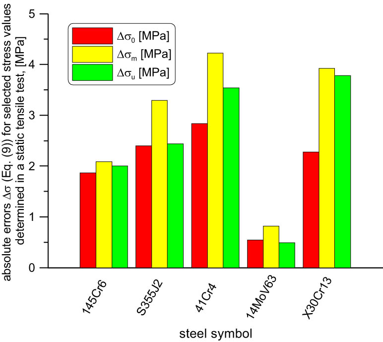
Comparison of the absolute errors Δσ for selected stress values determined in the static tensile test using equation (9).

Figure 7

Comparison of the absolute errors Δσ including the compensation for individual errors of component quantities, for selected stress values using equation (10).

Figure 8

Comparison of the absolute errors Δε and ΔA for selected strain and elongation values determined in the static tensile test using equation (9).

Figure 9

Comparison of the absolute errors Δε and ΔA including the compensation for individual errors of component quantities, for selected strain and elongation values using equation (10).

Figure 10

Comparison of the relative errors δσ for selected stress values determined in the static tensile test using equations (9) and (5).

Figure 11

Comparison of the relative errors δσ including the compensation for individual errors of component quantities, for selected stress values using equations (10) and (5).

Figure 12

Comparison of the relative errors δε and ΔA for selected strain and elongation values determined in the static tensile test using equations (9) and (5).

Figure 13

Comparison of the relative errors δε and ΔA including the compensation for individual errors of component quantities, for selected strain and elongation values using equations (10) and (5).

4 Discussion

The error values calculated using the compensation method are generally slightly lower than the error values calculated using the total differential method. Despite the low accuracy of the selected measuring tools, the absolute and relative error values obtained can be considered acceptable. Certainly, the introduction of error calculations into engineering practice in the field of laboratory measurements may seem natural; however, as noted at the beginning of this article, this is not shown in scientific papers. Although such analyzes are found in typical papers in the field of metrology of geometrical quantities and angle, they are difficult to find in scientific papers dealing with the subject of determining physical quantities considered as material constants or material characteristics. Perhaps this is due to the fact that the entire analysis scheme is based on painstaking calculations in the field of differential calculus, and this seems to be time consuming and labor intensive.

However, it is suggested that the research practice be consistent with the canons of science to give results of error calculus, which certainly says a lot about the accuracy of measuring physical quantities. The analysis can be simplified by using the Mathcad package or equivalent to automate calculations, as shown in this article. The authors do not exclude the development of an application that allows estimating the level of uncertainty in a static tensile test after entering the relevant data. The author of this article intends to refer the presented method of estimating measurement errors to other tests in the field of structural strength – for example, fracture mechanics or material fatigue.

That is why, in the Appendix, the author shows the method of determining the measurement uncertainty of the hardening exponent n in the power law (equation (12)). In the future, author plans to include the impact of measurement error of the strain hardening exponent value into account on the results obtained during the FEM calculations in the field of elastic–plastic fracture mechanics.

Funding information: This research was funded by the Faculty of Mechatronics and Mechanical Engineering at the Kielce University of Technology under the order number 01.0.09.00/2.01.01.00.0000 SUBB.MKMT.21.003.
Author contributions: M. G.: conceptualization, methodology, software, validation, formal analysis, investigation, resources, data curation, writing – original draft preparation, writing – review and editing, visualization, supervision, project administration, funding acquisition.
Conflict of interest: The author declares no conflict of interest.

Appendix A: Calculation of the uncertainty of the strain hardening exponent

It seems much more complicated to estimate the uncertainty of measurement of a power exponent in the RO law (equation (11)) or in the power law described by the formula (12), which, taking into account the assumption that the strengthening constant α = 1, is quite often used for approximation stress–strain curve by many researchers, including the author of this publication. Generally, based on two points – the yield strength and tensile strength (as well as the corresponding deformations), the strengthening exponent n assuming that the constant α = 1 is determined using formula (13). The determined value of the strain hardening exponent n determines the tensile curve used in the FEM numerical calculations, which in turn affects, as has already been mentioned, the value of the J-integral calculated numerically, or the level of stress near the crack tip, if you consider issues in the field of fracture mechanics, as shown in ref. [19].

In view of this fact, it was decided to include in the Appendix the calculation scheme carried out in the Mathcad package, which allows estimating the uncertainty of the measurement of the strain hardening exponent n in the power law described by the formula (12).

By using the “solve” function available in Mathcad, we automatically obtain the formula (13), using the second part of the formula (13), applicable for points above the yield point on the real stress–strain curve (below are excerpts of the calculation sheet from the MathCad package):

n ≔ ε m ε 0 = σ m σ 0 n solve , n = ln ε m ε 0 ln σ m σ 0 .

As we can see, the exponent n is a function of four variables (σ ₀, σ _m, ε _0, and ε _m). In view of this fact, material constants determined for the steels used in refs. [9,10,11,12] will be used in further analysis, as well as the corresponding errors generally indicated as ΔW, which was shown earlier. In the next step, according to the theory in paragraph 1, the partial derivatives will be estimated:

δ n ε 0 = d d ε 0 n δ n ε m = d d ε m n δ n σ 0 = d d σ 0 n δ n σ m = d d σ m n ,

which can be written as follows:

δ n ε 0 = − 1 ε 0 ⋅ ln σ m σ 0 δ n ε m = 1 ε m ⋅ ln σ m σ 0 δ n σ 0 = ln ε m ε 0 σ 0 ⋅ ln σ m σ 0 2 δ n σ m = ln ε m ε 0 σ m ⋅ ln σ m σ 0 2 .

In the next step, we can save the final formulas for relative and absolute errors made in determining the exponent n, both without and with compensation for component errors:

Relative error (equation (9)):
Δ n = ∣ δ n ε 0 ∣ ⋅ Δ ε 0 + ∣ δ n ε m ∣ ⋅ Δ ε m + ∣ δ n σ 0 ∣ ⋅ Δ σ 0 + ∣ δ n σ m ∣ ⋅ Δ σ m Δ n = Δ ε 0 ln σ m σ 0 ⋅ ∣ ε 0 ∣ + Δ ε m ln σ m σ 0 ⋅ ∣ ε m ∣ + Δ σ 0 ⋅ ln ε m ε 0 ln σ m σ 0 2 ⋅ ∣ σ 0 ∣ + Δ σ m ⋅ ln ε m ε 0 ln σ m σ 0 2 ⋅ ∣ σ m ∣ .
Absolute error (equations (9) and (5)):
δ n = Δ n ∣ n ∣ δ n = ln σ m σ 0 ⋅ Δ ε 0 ln σ m σ 0 ⋅ ∣ ε 0 ∣ + Δ ε m ln σ m σ 0 . ∣ ε m ∣ + Δ σ 0 ⋅ ln ε m ε 0 ln σ m σ 0 2 ⋅ ∣ σ 0 ∣ + Δ σ m ⋅ ln ε m ε 0 ln σ m σ 0 2 ⋅ ∣ σ m ∣ ln ε m ε 0 .
Relative error, taking into account individual errors of measured quantities (equation (10)):
Δ n = ( δ n ε 0 ⋅ Δ ε 0 ) 2 + ( δ n m ⋅ Δ ε m ) 2 + ( δ n σ 0 ⋅ Δ σ 0 ) 2 + ( ( δ n σ m ⋅ Δ σ m ) ) 2 Δ n = Δ ε 0 2 ε 0 2 ⋅ ln σ m σ 0 2 + Δ ε m 2 ε m 2 ⋅ ln σ m σ 0 2 + Δ σ 0 2 ⋅ ln ε m ε 0 2 σ 0 2 ⋅ ln σ m σ 0 4 + Δ σ m 2 ⋅ ln ε m ε 0 2 σ m 2 ⋅ ln σ m σ 0 4 .
Absolute error, taking into account individual errors of measured quantities (equations (10) and (5)):

δ n = Δ n ∣ n ∣ δ n = ln σ m σ 0 ⋅ Δ ε 0 2 ε 0 2 ⋅ ln σ m σ 0 2 + Δ ε m 2 ε m 2 ⋅ ln σ m σ 0 2 + Δ σ 0 2 ⋅ ln ε m ε 0 2 σ 0 2 ⋅ ln σ m σ 0 4 + Δ σ m 2 ⋅ ln ε m ε 0 2 σ m 2 ⋅ ln σ m σ 0 4 ln ε m ε 0 .

By using the algorithm shown earlier, for the steels considered in refs. [9,10,11,12], all absolute and relative error values were determined, and then, they were summarized in Table A1 and illustrated in Figure A1.

Table A1

The absolute and relative error values of strain hardening exponent n for steels used in this article

Steel	n	Δn	δn (%)	Δn	δn (%)
Steel	n	(Equations (9) and (5))		(Equations (10) and (5))
145Cr6	27.43	1.404	5.119	0.803	2.926
S355J2	6.90	0.309	4.48	0.163	2.367
41Cr4	9.69	0.525	5.415	0.286	2.950
14MoV63	9.16	0.232	2.536	0.154	1.676
X30Cr13	4.11	0.085	2.061	0.054	1.306

Figure A1

Comparison of the absolute and relative errors (denoted as Δn and δn, respectively) for strain hardening exponent n, for all steels used in this article.

Figure A2

Comparison of the real stress–strain curve determined for the estimated value of the strain hardening exponent and the curves drawn based on the strain hardening exponent reduced or increased by the value of absolute (example graph).

Figure A3

As can be seen, absolute and relative errors, estimated taking into account the compensation of individual errors of measured quantities (formulas (10) and (5)), are almost half smaller than errors determined in accordance with formulas (9) and (5). It can be stated that the higher the value of the strain hardening exponent (i.e., the lower the level of material hardening), the greater the measurement uncertainty value. The more brittle the material – the small value of the strain hardening exponent n, the smaller the uncertainty of measurement of this quantity. It can be arbitrarily stated that for the materials considered in this article, tested in the same laboratory conditions, with the same instruments (testing machine, extensometer, calliper), smaller errors in the determination of the strain hardening exponent n depending on the tensile curve obtained in the laboratory are observed for strongly hardening materials. An increase in the value of the strain hardening exponent results in a decrease in the hardening of the material and generates an increase in measurement uncertainty when determining this quantity.

The analysis of the assessment of measurement uncertainty in determining the strain hardening exponent n, carried out by the author for the purposes of this article, for the materials considered in this article indicates that above the yield point, the stress–strain curve may differ by several percent (Figures A2 and A3). In the summary presented in Figures A2 and A3, the difference between the model real curve determined for the estimated value of the strain hardening exponent and the curves drawn based on the strain hardening exponent reduced or increased by the value of absolute error, corresponding to the tensile strength, is more than 2%.

Appendix B: A list of formulas helpful in assessing the measurement uncertainty

Appendix B presents a list of all formulas derived during the preparation of this article, which may prove helpful in assessing the measurement uncertainty of the quantities determined during the uniaxial tensile test. These formulas were derived with the use of the MathCad package, using the symbolic calculation module.

Table B1

Determination of the absolute and relative error values of strain hardening exponent n for steels used in this article

Estimation of the measurement uncertainty of the stress quantity σ for a specimen with a rectangular cross-section
Equations (9) and (5)	Δ σ = Δ F ∣ a 0 ∣ ⋅ ∣ b 0 ∣ + Δ a 0 ⋅ ∣ F ∣ ( ∣ a 0 ∣ ) 2 ⋅ ∣ b 0 ∣ + Δ b 0 ⋅ ∣ F ∣ ∣ a 0 ∣ ⋅ ( ∣ b 0 ∣ ) 2
	δ σ = ∣ a 0 ∣ ⋅ ∣ b 0 ∣ ⋅ Δ F ∣ a 0 ∣ ⋅ ∣ b 0 ∣ + Δ a 0 ⋅ ∣ F ∣ ( ∣ a 0 ∣ ) 2 ⋅ ∣ b 0 ∣ + Δ b 0 ⋅ ∣ F ∣ ∣ a 0 ∣ ⋅ ( ∣ b 0 ∣ ) 2 ∣ F ∣
Equations (10) and (5)	Δ σ = Δ F 2 a 0 2 ⋅ b 0 2 + F 2 ⋅ Δ a 0 2 a 0 4 ⋅ b 0 2 + F 2 ⋅ Δ b 0 2 a 0 2 ⋅ b 0 4
	δ σ = ∣ a 0 ∣ ⋅ ∣ b 0 ∣ ⋅ Δ F 2 a 0 2 ⋅ b 0 2 + F 2 ⋅ Δ a 0 2 a 0 4 ⋅ b 0 2 + F 2 ⋅ Δ b 0 2 a 0 2 ⋅ zb 0 4 ∣ F ∣
Estimation of the measurement uncertainty of the stress quantity σ for a specimen with a circular cross-section
Equations (9) and (5)	Δ σ = 4 ⋅ Δ F π ⋅ ( ∣ d 0 ∣ ) 2 + 8 ⋅ Δ d 0 ⋅ ∣ F ∣ π ⋅ ( ∣ d 0 ∣ ) 3
	δ σ = π ⋅ ( ∣ d 0 ∣ ) 2 ⋅ 4 ⋅ Δ F π ⋅ ( ∣ d 0 ∣ ) 2 + 8 ⋅ Δ d 0 ⋅ ∣ F ∣ π ⋅ ( ∣ d 0 ∣ ) 3 4 ⋅ ∣ F ∣
Equations (10) and (5)	Δ σ = 4 ⋅ Δ F 2 π 2 ⋅ d 0 4 + 4 ⋅ F 2 ⋅ Δ d 0 2 π 2 ⋅ d 0 6
	δ σ = π ⋅ ( ∣ d 0 ∣ ) 2 ⋅ Δ F 2 π 2 ⋅ d 0 4 + 4 ⋅ F 2 ⋅ Δ d 0 2 π 2 ⋅ d 0 6 ∣ F ∣
Estimation of the measurement uncertainty of the quantity being a contraction Z for a specimen with a rectangular cross-section
Equations (9) and (5)	Δ Z = Δ a 0 ⋅ 1 a 0 + a ⋅ b − a 0 ⋅ b 0 a 0 2 ⋅ b 0 + Δ b 0 ⋅ 1 b 0 + a ⋅ b − a 0 ⋅ b 0 a 0 ⋅ b 0 2 + Δ b ⋅ ∣ a ∣ ∣ a 0 ∣ ⋅ ∣ b 0 ∣ + Δ a ⋅ ∣ b ∣ ∣ a 0 ∣ ⋅ ∣ b 0 ∣
	δ Z = ∣ a 0 ∣ ⋅ ∣ b 0 ∣ ⋅ Δ a 0 ⋅ 1 a 0 + a ⋅ b − a 0 ⋅ b 0 a 0 2 ⋅ b 0 + Δ b 0 ⋅ 1 b 0 + a ⋅ b − a 0 ⋅ b 0 a 0 ⋅ b 0 2 + Δ b ⋅ ∣ a ∣ ∣ a 0 ∣ ⋅ ∣ b 0 ∣ + Δ a ⋅ ∣ b ∣ ∣ a 0 ∣ ⋅ ∣ b 0 ∣ ∣ a ⋅ b − a 0 ⋅ b 0 ∣
Equations (10) and (5)	Δ Z = Δ a 0 2 ⋅ 1 a 0 + a ⋅ b − a 0 ⋅ b 0 a 0 2 ⋅ b 0 2 + Δ a b 0 2 ⋅ 1 b 0 + a ⋅ b − a 0 ⋅ b 0 a 0 ⋅ b 0 2 2 + a 2 ⋅ Δ b 2 a 0 2 ⋅ b 0 2 + b 2 ⋅ Δ a 2 a 0 2 ⋅ b 0 2
	δ Z = ∣ a 0 ∣ ⋅ ∣ b 0 ∣ ⋅ Δ a 0 2 ⋅ 1 a 0 + a ⋅ b − a 0 ⋅ b 0 a 0 2 ⋅ b 0 2 + Δ a b 0 2 ⋅ 1 b 0 + a ⋅ b − a 0 ⋅ b 0 a 0 ⋅ b 0 2 2 + a 2 ⋅ Δ b 2 a 0 2 ⋅ b 0 2 + b 2 ⋅ Δ a 2 a 0 2 ⋅ b 0 2 ∣ a ⋅ b − a 0 ⋅ b 0 ∣
Estimation of the measurement uncertainty of the quantity being a contraction Z for a specimen with a circular cross-section
Equations (9) and (5)	Δ Z = Δ d 0 ⋅ 2 d 0 + 2 ⋅ π ⋅ d 2 − 2 ⋅ π ⋅ d 0 2 π ⋅ d 0 3 + 2 ⋅ Δ d ⋅ ∣ d ∣ ( ∣ d 0 ∣ ) 2
	δ Z = π ⋅ ( ∣ d 0 ∣ ) 2 ⋅ Δ d 0 ⋅ 2 d 0 + 2 ⋅ π ⋅ d 2 − 2 ⋅ π ⋅ d 0 2 π ⋅ d 0 3 + 2 ⋅ Δ d ⋅ ∣ d ∣ ( ∣ d 0 ∣ ) 2 ∣ π ⋅ d 2 − π ⋅ d 0 2 ∣
Equations (10) and (5)	Δ Z = Δ d 0 2 ⋅ 2 d 0 + 2 ⋅ π ⋅ d 2 − 2 ⋅ π ⋅ d 0 2 π ⋅ d 0 3 + 4 ⋅ d 2 ⋅ Δ d 2 d 0 4
	δ Z = π ⋅ ( ∣ d 0 ∣ ) 2 ⋅ Δ d 0 2 ⋅ 2 d 0 + 2 ⋅ π ⋅ d 2 − 2 ⋅ π ⋅ d 0 2 π ⋅ d 0 3 + 4 ⋅ d 2 ⋅ Δ d 2 d 0 4 ∣ π ⋅ d 2 − π ⋅ d 0 2 ∣
Estimation of the measurement uncertainty of the quantity which is the strain ε
Equations (9) and (5)	Δ ε = Δ l 0 ⋅ − 1 l 0 − l − l 0 l 0 2 + l ∣ l 0 ∣
	δ ε = ∣ l 0 ∣ ⋅ Δ l 0 ⋅ − 1 l 0 − l − l 0 l 0 2 + l ∣ l 0 ∣ ∣ l − l 0 ∣
Equations (10) and (5)	Δ ε = Δ l 0 2 ⋅ 1 l 0 + l − l 0 l 0 2 2 + Δ l 2 l 0 2
	δ ε = ∣ l 0 ∣ ⋅ Δ l 0 2 ⋅ 1 l 0 + l − l 0 l 0 2 2 + Δ l 2 l 0 2 ∣ l − l 0 ∣
Estimation of the measurement uncertainty of the quantity, which is the elongation A
Equations (9) and (5)	Δ A = Δ l + Δ l 0
	δ A = Δ l + Δ l 0 ∣ l − l 0 ∣
Equations (10) and (5)	Δ A = Δ l 2 + Δ l 0 2
	δ A = Δ l 2 + Δ l 0 2 ∣ l − l 0 ∣
Estimation of the measurement uncertainty of the strain hardening exponent n in the power law – formula (12) for the power constant α = 1
Equations (9) and (5)	Δ n = Δ ε 0 ln σ m σ 0 ⋅ ∣ ε 0 ∣ + Δ ε m ln σ m σ 0 ⋅ ∣ ε m ∣ + Δ σ 0 ⋅ ln ε m ε 0 ln σ m σ 0 2 ⋅ ∣ σ 0 ∣ + Δ σ m ⋅ ln ε m ε 0 ln σ m σ 0 2 ⋅ ∣ σ m ∣
	δ n = ln σ m σ 0 ⋅ Δ ε 0 ln σ m σ 0 ⋅ ∣ ε 0 ∣ + Δ ε m ln σ m σ 0 ⋅ ∣ ε m ∣ + Δ σ 0 ⋅ ln ε m ε 0 ln σ m σ 0 2 ⋅ ∣ σ 0 ∣ + Δ σ m ⋅ ln ε m ε 0 ln σ m σ 0 2 ⋅ ∣ σ m ∣ ln ε m ε 0
Equations (10) and (5)	Δ n = Δ ε 0 2 ε 0 2 ⋅ ln σ m σ 0 2 + Δ ε m 2 ε m 2 ⋅ ln σ m σ 0 2 + Δ σ 0 2 ⋅ ln ε m ε 0 2 σ 0 2 ⋅ ln σ m σ 0 4 + Δ σ m 2 ⋅ ln ε m ε 0 2 σ m 2 ⋅ ln σ m σ 0 4
	δ n = ln σ m σ 0 ⋅ Δ ε 0 2 ε 0 2 ⋅ ln σ m σ 0 2 + Δ ε m 2 ε m 2 ⋅ ln σ m σ 0 2 + Δ σ 0 2 ⋅ ln ε m ε 0 2 σ 0 2 ⋅ ln σ m σ 0 4 + Δ σ m 2 ⋅ ln ε m ε 0 2 σ m 2 ⋅ ln σ m σ 0 4 ln ε m ε 0

σ – stress; σ ₀ – yield stress; σ _m – ultimate strength; ε – strain; ε ₀ – strain corresponding to the yield stress; ε _m – strain corresponding to the ultimate strength; α – strain hardening constant in power law equation (12) – in this calculation α = 1; n – strain hardening exponent in power law equation (12); F – force; a ₀, b ₀ – initial dimensions of the specimen with rectangular cross-section (a ₀ and b ₀); a, b – final dimensions of the specimen with rectangular cross-section (a and b); d ₀ – initial diameter of the specimen with circular cross-section (π·d ₀ ²/4); d – final diameter of the specimen with circular cross-section (π·d ²/4); A – elongation of the specimen; Z – contraction of the specimen.

References

1 PN-EN ISO 6892-1:2016-09. Metals – Tensile test – Part 1: test method at room temperature; 2016 (Polish).Search in Google Scholar

2 ASTM E8/E8M − 13a. Standard test methods for tension testing of metallic materials; 2013.Search in Google Scholar

3 SINTAP – Structural Integrity Assessment Procedures for European Industry. Final procedure. Brite-Euram project no. BE95-1426. Rotherham: British Steel; 1999.Search in Google Scholar

4 Kocak M, Webster S, Janosch JJ, Ainsworth RA, Koers R. FITNET report – European fitness-for-service network. Edited by contract no. G1RT-CT-2001-05071; 2006.Search in Google Scholar

5 Neimitz A, Dzioba I, Graba M, Okrajni J. The assessment of the strength and safety of the operation high temperature components containing crack. Kielce: Kielce University of Technology Publishing House; 2008 (Polish).Search in Google Scholar

6 Rumszyski LZ. Mathematical preparation of the results of the experiment. Warsaw: WNT; 1973 (Polish).Search in Google Scholar

7 Greń J. Mathematical statistics. Warsaw: PWN; 1987 (Polish).Search in Google Scholar

8 Klonecka W. Statistics for engineers. Warsaw: PWN; 1999. (in Polish).Search in Google Scholar

9 Graba M. Experimental and numerical assessment of elasto-plastic parameters of fracture mechanics for 145Cr6 steel. Part I. Mech Rev. 2013;4:31–8 (Polish).Search in Google Scholar

10 Graba M. About problems in determining selected mechanical properties of 41Cr4 steel. Mechanik. 2016;8–9:974–53 (Polish).10.17814/mechanik.2016.8-9.331Search in Google Scholar

11 Graba M. Maximum crack opening stresses as a parameter controlling the fracture process. Proceedings of the XXIII Symposium of Fatigue and Fracture Mechanics. Bydgoszcz – Pieczyska. 1; 2010. p. 1–13 (Polish).Search in Google Scholar

12 Neimitz A, Dzioba I, Molasy R, Graba M. The influence of constarints on the fracture toughness of brittle materials. Proceedings of the XX Symposium of Fatigue and Fracture Mechanics. Bydgoszcz-Pieczyska. 1; 2004. p. 265–72 (Polish).Search in Google Scholar

13 Hutchinson JW. Singular behaviour at the end of a tensile crack in a hardening material. J Mech Phys Solids. 1968;16:13–31.10.1016/0022-5096(68)90014-8Search in Google Scholar

14 Graba M. Proposal of the hybrid solution to determining the selected fracture parameters for SEN(B) specimens dominated by plane strain. Bull Pol Acad Sci Technical Sci. 2017;65(4):523–32.10.1515/bpasts-2017-0057Search in Google Scholar

15 Graba M. The influence of material properties on the Q-stress value near the crack tip for elastic-plastic materials. J Theor Appl Mech. 2008;46(2):269–90.Search in Google Scholar

16 Graba M. Catalogue of the numerical solutions for SEN(B) specimen assuming the large strain formulation and plane strain condition. Arch Civ Mech Eng. 2012;12(1):29–40.10.1016/j.acme.2012.03.005Search in Google Scholar

17 Neimitz A, Graba M. Analytical-numerical hybrid method to determine the stress field in front of the crack in 3D elastic-plastic structural elements. Proceedings of XVII ECF. Brno – Czech Republic. Article in the electronic form, abstract – book of abstracts; 2008. p. 85.Search in Google Scholar

18 Graba M. Numerical analysis of the influence of in-plane constraints on the crack tip opening displacement for SEN(B) specimens under predominantly plane strain conditions. Int J Appl Mech Eng. 2016;21(4):849–66.10.1515/ijame-2016-0050Search in Google Scholar

19 Graba M, Neimitz A. On methods of determining material parameters in the Ramberg-Osgood law. Proceedings of the X Polish Conference of Fracture Mechanics. Opole – Wisła. 1; 2005. p. 323–32 (Polish).Search in Google Scholar

Received: 2021-01-21

Revised: 2021-03-29

Accepted: 2021-04-13

Published Online: 2021-05-18

This work is licensed under the Creative Commons Attribution 4.0 International License.

Articles in the same Issue

https://doi.org/10.1515/eng-2021-0069

Keywords for this article

static tensile test; measurement uncertainty; absolute error; relative error; material constant; mechanical properties

Creative Commons

BY 4.0