Prediction of future paths of mobile objects using path library

Helena Leppäkoski; Bishwo Adhikari; Leevi Raivio; Risto Ritala

doi:10.1515/eng-2021-0103

Article Open Access

Prediction of future paths of mobile objects using path library

Helena Leppäkoski , Bishwo Adhikari , Leevi Raivio and Risto Ritala

Published/Copyright: November 8, 2021

Published by

Become an author with De Gruyter Brill

Submit Manuscript Author Information

From the journal Open Engineering Volume 11 Issue 1

Abstract

In situational awareness, the ability to make predictions about the near future situation in the area under surveillance is often as essential as being aware of the current situation. We introduce a privacy-preserving instance-based prediction method, where a path library is collected by learning earlier paths of mobile objects in the area of surveillance. The input to the prediction is the most recent coordinates of the objects in the scene. Based on similarity to short segments of currently tracked paths, a relative weight is associated with each path in the library. Future paths are predicted by computing the weighted average of the library paths. We demonstrate the operation of a situational awareness system where privacy-preserving data are extracted from an inexpensive computer vision which consists of a camera-equipped Raspberry PI-based edge device. The system runs a deep neural network-based object detection algorithm on the camera feed and stores the coordinates, object class labels, and timestamps of the detected objects. We used probabilistic reasoning based on joint probabilistic data association, Hungarian algorithm, and Kalman filter to infer which detections from different time instances came from the same object.

Keywords: path prediction; people tracking; probabilistic data association; instance-based learning; computer vision

1 Introduction

The current developments in camera technologies and deep-learning-based signal processing have made computer vision systems cost-effective and feasible options for various surveillance tasks. In many applications, the ability to make predictions about the near future situation in the area under surveillance is as essential as being aware about current situation. For example, the security of the working environment of mobile machinery could be improved by a vision system that automatically detects objects in the area, predicts locations of the mobile objects, and determines how probably some parts of the area will be occupied in the near future. The ability to predict future locations allows, e.g., prediction of possible congestion in crowded areas or observation of atypical movement behaviors. For the operator of mobile machinery, the timely warnings provided with the help of these kinds of predictions could allow extra time to react when nearby mobile objects are about to enter to area of safety risk by approaching too close.

In this article, we introduce an instance-based prediction method, where a path library is collected by learning earlier paths of mobile objects in the area of surveillance, which preserves privacy of the tracked people. Many existing computer vision systems for surveillance rely on transmitting or storing video data to servers for further analysis. This compromises personal privacy of the people in the area. In our method, only position coordinates of the detected moving objects and the detection timestamps need to be extracted from the camera data. Any data that might identify the individuals are not stored or saved to the server.

We demonstrate the operation of a situational awareness system that uses only privacy-preserving data extracted from the computer vision system to track paths, learn the path library, and predict paths with the path library. Our system uses the limited set of data to answer the following questions: Are there people in the surveillance area? If there are, where are they and what kind of paths are they taking? Where will they be located, and which parts of the area will probably be occupied in the near future?

This article is organized as follows. Section 2 gives a brief summary of the reported work related to the topic and contents of this article. In Section 3, signal processing and algorithmic methods are described: processing of the camera-based observations to position coordinates, path tracking from time tagged coordinate samples, construction of the path library from the tracked paths, and using the recorded paths from the path library to predict the future paths of the moving objects in the camera scene. Section 4 describes the experimental setup to demonstrate the path prediction method, and finally in Sections 5–7 the results are reported and discussed and conclusions of the work are given.

2 Related work

The extension of Kalman filter (KF) techniques to prediction is a well-known approach [1]. Typically, the role of the KF in prediction is to propagate the system’s state estimate and its covariance in time using the system’s dynamic model that is represented in the form suitable for KF propagation equations. In some applications, the initial data sequence from the system is processed with the KF to obtain an accurate estimate of the initial state, from which the prediction can be started. For example, this approach is used in ref. [2] to predict the orbits of navigation satellites for 4 days ahead. Similarly, in our work we use the KF for initialization of both the library-based prediction and the KF prediction. However, the used models are different and in our work, other supporting methods, such as object detection and data association (DA), were required.

For pedestrian motion prediction from video stream, Schöller et al. [3] compared the prediction accuracy of simple constant velocity model without random perturbations to several state-of-the-art neural networks, e.g., long short-term memories (LSTMs), LSTM with state refinement (SR-LSTM), feed forward neural network, and social generative adversarial network (S-GAN). The conclusion of ref. [3] is that the simple model outperforms the neural networks in this task. Our work aims to solve the same problem, however, with different constraints (e.g., need for DA and randomly varying observation sampling) and targets to longer prediction lengths, and therefore we also use different methods. While in ref. [3] the number of time steps for initial observations and prediction lengths is 8 and 12, corresponding the time windows of 3.2 and 4.8 s, in our tests the length of the initial observation is 5–7 s (and samples) and the prediction lengths are 4–6, 9–11, and 19–21 s (and samples). We also enhance our prediction model by a collection of past paths stored into path library. The path library can be seen as an instance-based or memory-based learning method, a nonparametric method that uses the training instances themselves as a model [4].

Yrjanainen et al. [5] presented privacy-aware person tracking and counting on Raspberry Pi edge device together with the neural computing stick for smooth computation. They used object detection, person re-identification, tracking, and counting on the edge device and collected encrypted information over the network. However, while ref. [5] used a set of abstract features to identify the detected individuals, in this work, we did not use any individual identifying data at all. We deploy an object detection network on Raspberry Pi to collect only the object locations and the detection timestamps.

3 Methods

The path prediction using path library consists of several tasks. The tasks and the structure of their mutual connections are depicted in Figure 1.

Figure 1

Main functional blocks of the path prediction system.

First, the typical paths need to be learned, i.e., the path library needs to be collected. From camera images, the objects need to be detected and their locations estimated to obtain samples that include the coordinates of the detected objects and the timestamps of the detections. Without any data elements that identify the objects, it is not obvious which detections come from which objects. The missing link between the distinct samples is estimated by solving the DA problem: a new detection needs either to be associated with one of the existing tracked paths or to be found not to be a part of any of them, in which case it is treated as a start of a new path.

Once we know to which path the new detection is associated, we can track the path, i.e., use the position of the detection to update the path. We treat the path tracking task as a state estimation problem, where the motion model represents our assumptions on what kind of movements and motion changes are possible, i.e., what is the inertia of the object. We store the information on tracked paths to a database, which we call path library. A stored path is a sequence of positions and their estimated uncertainties.

To use the paths stored in the library for prediction, we need information on which paths might be relevant for the situation. To obtain that information, we need to run the path tracking to get an initial idea of what is happening in the camera scene. Once we have tracked a new path for a couple of time steps, this short path segment can be compared with the contents of the path library. The library paths most similar to the new segment can be used to predict the future path. In the following subsections, these tasks are described in detail.

3.1 Object detection

The first step is to find the bounding boxes associated with the objects in the camera view. For object detection, convolutional neural network (CNN)-based methods have been proven to be effective with their state-of-the-art performances on public benchmark datasets [6,7, 8,9]. These CNN-based object detection methods can be broadly divided into two groups: one-stage and two-stage. One-stage detectors are efficient and have straightforward architecture. In contrast, two-stage detectors have complicated architecture but perform better in terms of detection accuracy. Given an input image, the one-stage method directly outputs the object location and class without an intermediate proposal. The two-stage method explicitly generates region proposals followed by feature extraction, category classification, and finetuning of the location proposals. Single-Shot MultiBox Detector (SSD) [7], YOLO3 [6], and RetinaNet [8] are commonly used one-stage neural network solutions. Regional CNNs (RCNNs) [10] such as faster RCNN [9] and mask RCNN [11] are commonly used two-stage detectors.

For the detection, we use pretrained weights from the network trained on MSCOCO [12] and the fine-training of the network with our custom dataset, collected from our test environment mentioned in Section 4.2. Our Raspberry Pi system contains a single-stage object detection network, SSD MobileNetV2, that predicts object locations and a pre-defined class category for each detection. We then save object locations and class labels together with detection timestamps.

Since the data were captured with a stationary monocular camera, depth and – consequently – the distance of detected objects from the camera are unknown. Therefore, the three-dimensional locations of detected objects cannot be acquired directly. To estimate their location on the map, the objects are assumed to lie on a planar surface. A linear transformation is fitted by minimizing the Euclidean distance between known map points and estimates based on their respective positions in the image. Essentially, points in the image plane are transformed to a plane representing the ground surface and scaled to map coordinates. Objects are then projected to the map by applying the transformation to the center point between the two bottom corners of their bounding boxes, i.e., the part most likely to be connected to the ground. The camera is calibrated before the fitting procedure, and images are rectified before object detection and transformations. Although the transformation procedure is relatively simple, it works well in this study because the area in question is relatively small and flat.

3.2 Path estimation

An overview of the tasks involved in the path estimation and its data flow is shown in Figure 2. The basic tool in the path estimation is KF, which is described in many textbooks, e.g., in ref. [13,14]. The probabilistic reasoning for the DA uses the KF predictions, and the results of the DA are used in the KF state update. We presented the position coordinates of the detections and path points in local-level-system and its east-north-up (ENU) version [1]. As we assumed the objects to be located in a horizontal plane, we omitted the vertical coordinate. In the following, we denote the east and north coordinates as x and y , respectively.

Figure 2

Subtasks of probabilistic reasoning for path estimation.

3.2.1 System model

In the KF, we use constant velocity model as motion model to propagate the path estimates in time. The model consists of four states: position coordinates and velocities in two dimensions, written as x k = [ x ( k ) , y ( k ) , v x ( k ) , v y ( k ) ] T . The state is driven by zero-mean, Gaussian acceleration w ( k ) . The discrete-time representation of the model is derived according to ref. [13]:

(1) x ( k ) = F x ( k − 1 ) + w ( k − 1 ) , k = 1 , … F = 1 0 Δ T 0 0 1 0 Δ T 0 0 1 0 0 0 0 1

where the variance of the driving noise w ( k ) is

(2) E [ w ( k ) w ( i ) T ] = Q , i = k 0 , i ≠ k , Q = Δ T 3 3 0 Δ T 2 2 0 0 Δ T 3 3 0 Δ T 2 2 Δ T 2 2 0 Δ T 0 0 Δ T 2 2 0 Δ T σ w 2 ,

σ w 2 is the variance of the driving noise, Δ T is the sampling time, and k is the index of the sampling instance. This model suits well for pedestrian motion, which forms the majority of the motion observed in our test environment. Other motion models that better describe the motion of objects with larger inertia and higher dynamics can be found, e.g., in publication [P1] of ref. [15].

The observation model is used for updating the path estimate. It describes the relationship between the true position of the object and the location of the detected object in the camera image projected onto map coordinates:

(3) z ( k ) = H x ( k ) + v ( k ) , k = 1 , … H = 1 0 0 0 0 0 1 0

where the variance of the measurement noise v ( k ) is

(4) E [ v ( k ) v ( i ) T ] = R , i = k 0 , i ≠ k .

In our system, we used the following parameter values: Δ T = 1 s and σ w 2 = 0.35 4 2 . As we had chosen the map coordinates so that the pointing angle of the camera was roughly to the direction of the negative x axis, and the projection of image coordinates to map coordinates is less accurate in the depth than width direction, we used higher variance for the x detection:

R = 4 0 0 1 .

The choice of the values of covariances Q and R was based on our prior knowledge about the system, i.e., they were not systematically optimized or fitted to the data.

3.2.2 DA and path update

As the data did not include elements that link the latest detections to the earlier detections from the same object, we formed the link computationally as a solution of DA problem. For this task, we used joint probabilistic data association (JPDA), a well-known method in, e.g., radar-based surveillance systems [16].

The first step of JPDA is the validation of the detections, where the task is to find which detected positions z j ( k ) , j = 1 , … , n z ( k ) are valid candidates to be associated with the existing paths, represented by their time-propagated estimates x ˆ i ( k ∣ k − ℓ ) , i = 1 , … , n x ( k ) . Here ℓ is the number of time steps the estimate is projected ahead after its last observation-based update, n z ( k ) and n x ( k ) are the numbers of detections and active paths at time index k , respectively.

The detection j is considered to be a valid association candidate to path i , if its observation likelihood with the path exceeds threshold P G . As we assume that the errors of the detection positions and the path estimation errors are Gaussian, the validation region, i.e., the area where the likelihood condition holds, is an ellipse (illustrated in Figure 3). Its center is located in the position coordinates of the predicted path, x ˆ i ( k ∣ k − ℓ ) , and its size and shape are defined by the covariance matrix of the error between the predicted observation z ˆ i ( k ) = H x ˆ i ( k ∣ k − ℓ ) and the actual observation z j . Therefore, the innovation covariance S i ( k ∣ k − ℓ ) = H P i ( k ∣ k − ℓ ) H T + R is computed for each path i and innovation vector z ˜ i , j ( k ) = z j ( k ) − z ˆ i ( k ) is computed for all pairs of paths i and detections j .

Figure 3

Example of validation regions. The four latest detections (the circles) and the elliptic validation regions of two paths. The crosses denote the path estimates updated by their associated detections and the predicted path positions based are shown with squares.

For Gaussian vectors, the checking against a probability threshold with probability ellipses can be transformed to checking of Mahalanobis distances. The squared Mahalanobis distance of innovation is d i , j 2 ( k ) = z ˜ i , j ( k ) T ( S i ( k ∣ k − ℓ ) ) − 1 z ˜ i , j ( k ) . For a Gaussian 2D vector, the Mahalanobis distance follows χ 2 ( 2 ) distribution. Therefore, instead of checking whether a point lies inside a probability ellipse, we can check that the Mahalanobis distance between the point and the center of the ellipse does not exceed the corresponding d 2 threshold. This threshold is obtained from χ 2 ( 2 ) inverse cumulative distribution function: d P G 2 = F χ 2 ( 2 ) − 1 ( P G ) . In our experiments, we used P G = 0.99 and the corresponding d P G 2 = 9.21 .

Based on the computed Mahalanobis distances, all detections z j ′ for which d i ′ , j ′ 2 ( k ) ≤ d P G 2 are considered valid association candidates for paths x ˆ i ′ . However, these are not necessarily correct associations, as there may be several detections in validation region or there may be overlapping validation regions when two or several paths share common candidates. It is also possible that more than one path have the shortest Mahalanobis distance to the same detection.

The next task is to find the association between the detections that are valid association candidates and the paths that have valid candidates in their validation regions. When assigning the detections to the paths, we allow at most one detection to be associated with at most one path, i.e., for each path and each detection, there is either one-to-one association or no association at all. We want to find the matching pairs so that the overall cost, i.e., the sum of the squared Mahalanobis distances between the associated detections and paths, is minimized. This type of linear assignment problem can be solved with Hungarian algorithm [17,18]. We used Matlab function matchpairs to solve the problem.

Once the association between the detections and path estimates is made, we run the KF observation update for the path estimates that have an associated detection. Often there are also detections that are not associated with a path, either because they were not valid candidates or because there were more valid association candidates than active path estimates. We treat these detections as initial observations of new paths. After all the detections are used to update either an existing or a new path, the path estimates are propagated in time using the motion model defined in (1) and (2), until new detections are available.

After the propagation steps, the uncertainties of the path estimates are checked. The product of the eigenvalues of the position covariance is computed and if it exceeds the uncertainty threshold, the path is removed from the set of active path estimates.

3.3 Path library

In the training phase of the prediction model, the paths removed from the set of active paths are stored into path library. For each path, the sequence of path position estimates and the corresponding covariance matrices were stored. To prevent too short-lived path sequences from populating the library, we did not store sequences that were shorter than the threshold L pmin . The sequence length was defined as the difference between the last and first observation update of the path estimate. For the sampling instances without observation update, the predicted estimate was stored, otherwise the updated estimate.

As we used only one camera, it is possible that an object may stay behind another object for several sampling instances, and has moved far from the edges of the camera view when it becomes visible for the camera for the first time. Therefore, we accept that a path can start everywhere in the camera view. Considering this condition, we added a grid representation into the path library to allow faster search of similar library paths in path prediction. We divided the area into 1 m × 1 m grid and to each grid cell, we stored the indices of the paths and the sequence indices of these paths that have coordinates located in the cell.

3.4 Prediction

The library-based prediction principle is illustrated in Figure 4. The input to library-based prediction is the most recent position coordinates of the objects in the scene. The paths are tracked from the detections with the KF model and JPDA techniques described in Section 3.2.2. When the lengths of such paths increase above a given threshold δ t min = n ip Δ T , the obtained path segment, which we call initial path, is compared to the contents of the path library.

Figure 4

The predicted path is the weighted sum of the most similar library paths.

Based on similarity with the initial path, a relative weight is associated with the paths of the library. However, to avoid giving any weight to the library paths very far away from the initial path and to save computational resources, we limit similarity comparisons using the grid representation of the library. We start scanning the library paths from the library grid cell where the initial path starts and then continue to the neighboring cells and further by increasing the distance to the starting cell, until the weights of n pmax library paths are evaluated or all the cells within the Manhattan distance d cmax to the starting cell have been checked.

The similarity between the paths is evaluated using the assumption of the Gaussian distribution of the path point coordinates and the common interpretation that the KF estimate and its covariance are the parameters of this distribution. In the following, an initial path and a library path are defined by sequences { μ ˆ ip ( k ) , Σ ip ( k ) } and { μ ˆ lib ( k ) , Σ lib ( k ) } , respectively, where k = 1 , … , n ip . Here μ ˆ and Σ represent the position parts of the estimate and its covariance, i.e., μ ˆ = x ˆ 1 : 2 and Σ = P 1 : 2 , 1 : 2 . First the Mahalanobis distances between the initial path and the library path are computed for k = 1 , … , n ip :

d ip,lib 2 ( k ) = ( μ ˆ ip ( k ) − μ ˆ lib ( k ) ) T ( Σ ip ( k ) + Σ lib ( k ) ) − 1 ( μ ˆ ip ( k ) − μ ˆ lib ( k ) ) .

From this, the corresponding values of χ 2 ( 2 ) probability distribution function are computed:

p ( k ) = f χ 2 ( 2 ) ( d ip,lib 2 ( k ) ) .

The weight of the library path is obtained as

(5) w ip,lib = exp ∑ k = 1 n ip log ( p ( k ) ) .

Using the weights (5), computed for all library paths that were found from the grid cells close to the start of the recently tracked initial path segment, the future path is predicted by computing the weighted average of the paths in the library and its uncertainty is expressed with its weighted covariance matrix. Quite commonly, the prediction is composed of several “branches,” meaning that the distribution of predicted agent’s location is multimodal. In this case, an appropriate descriptor of the uncertainty is the smoothed probability distribution produced by the Gaussian mixture that represents the branches.

If library paths that match closely enough with the initial path are not found, all the path weights are zeros and we cannot compute the library-based prediction. Then the algorithm has to revert to KF-based prediction as a fallback method.

In our experiments, we used the following parameter values: δ t min = n ip = 6 , n pmax = 50 , d cmax = 15 , and L pmin = n ip + n pred , where n pred is the number of time steps that the prediction is computed for.

4 Experiments

For real data demonstration, we collected camera-based object detections. We used part of the data to learn the paths to path library and another part to assess the quality of library-based prediction by comparing it to the KF-based prediction. In the following, we describe the hardware we used, the data we collected, and the test procedure for the prediction.

4.1 Hardware

We use affordable, portable, and easily available edge-device to collect experimental data and run the detection system. The system includes Raspberry Pi 3 Model B+ equipped with 8 Mpix Raspberry camera module V2. Cooling fan and heat sinks are attached to the Raspberry to prevent overheating and unexpected shutdown during continuous operation for days. The system shown in Figure 5 is placed on the fifth floor of the Tampere University Hervanta Campus building facing toward the open space next to the parking yard and capturing the view in Figure 6.

Figure 5

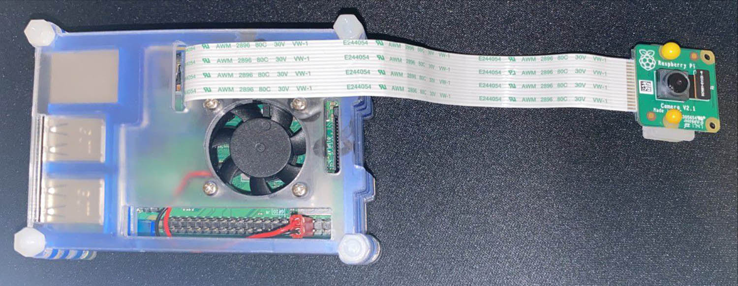
Hardware for the data collection and running detection network.

Figure 6

Camera view from the test setup running real time object detection on a Raspberry Pi platform.

4.2 Data

The system described in Section 4.1 was used to collect full HD videos during daylight in summer 2018. About 800 frames were extracted from videos captured on different days and times. These image frames were fully labeled in six class categories: bus, car, cyclist, person, truck, and van, using the technique mentioned in ref. [19]. One annotation means two coordinate points and a classification, visualized as a box and a written class label. The aim was to create a representative dataset including various moving objects during daylight for the object detection network training. We emphasize that our system does not send any visual data to the server. Once the detection system is online, it sends the detected object’s location coordinates and associated timestamps. However, we save some amount of visual data for system debugging and visualization purposes. Hence, the system preserves the privacy of the person being in the camera view.

In the dataset, “person” was the only category with plenty of instances spread over the scene. Therefore, we used only this category in the prediction tests. These detections appear in bursts and the intervals between the detection bursts vary randomly, the most common interval lengths being 2 or 3 s.

To create the path library, we used stored location and timestamp data collected on day 1 during 13 h. The data from the next day were used to compare the predictions produced by the path library and the traditional KF. The path tracking and prediction were implemented with Matlab.

4.3 Test procedure

In the prediction tests, we wanted to compare the predictions to the detections and to examine the performance of the method in different prediction lengths. We defined three interesting prediction lengths t pred = n pred Δ T : for short-, middle- and long-term predictions, t pred was 5 ± 1 , 10 ± 1 , and 20 ± 1 , respectively.

The random variation of the sampling interval posed challenges to the testing, as to be able to assess a prediction made for a time instance, there should be detections available at the time. To tackle this problem, we used the timing shown in Figure 7. The value δ t min = 6 s was chosen to make sure that most often at least three detection instances will be included in the initial path. To allow comparison against detections, the predictions were computed and saved for three time instances around the targeted prediction lengths. Due to the variation in the detection sample intervals, the actual tracking interval δ t varies as the tracking ends when the first detections are obtained such that δ t ( m ) ≥ δ t min . For the same reason, the age of the prediction that is compared with the actual detections also varies.

Figure 7

Timing diagram of the prediction test exemplifying the effect of the random variation of detection times.

In the test, we stopped the path tracking and cleared the memory of the initial path after it was used to compute predictions. The future detections, possibly originating from the same actual paths were then used to start and track a new initial path, i.e., the detections from the same actual path were used to start predictions several times at different phases of the path build-up.

We compared the predictions produced by the path library to the predictions of KF. With KF we mean here the same KF combined with JPDA that produced the initial path for library-based method, but instead of using the initial path, the KF used its last estimated state and the motion model (1) to make prediction for the next n pred time steps.

5 Results

To assess the capability of the library-based path prediction, it was compared to KF predictions. The criterion for the comparison was how probable the prediction method had considered the detection of objects in the location where they actually appeared. Looking at a location where an object became detected, the higher its predicted probability to be occupied was, the more successful we considered the prediction.

A captured moment of a tracking and prediction situation is shown in Figure 8. For illustration purposes, the build-up history of paths is shown even though for prediction, the path history was cleared after the predictions were computed. Some phenomena are marked with labels in the figure: (1) two adjacent paths; (2) a long, static sequence of detections; (3) a long path; (4) a short, static sequence of detections; (5) predictions indicate probable detections but the series of detections has ended; and (6) pink shade on the map denote areas where library paths have plenty of position occurrences. The expanding yellow circles represent the KF predictions and their uncertainty that increases with time. The blue circles represent the uncertainties of the library-based predictions, which do not expand to as large area as the uncertainties of the KF predictions but sometimes divide into different branches.

Figure 8

Real data example: path tracking and predictions with KF and path library.

To get more focused comparisons, we computed the short-, middle-, and long-term predictions as described in Section 4.3. The occupancy predictions plotted on the maps together with the detections are shown in Figure 9, where predictions for two time instances are given as examples. In the occupancy map, the darker the color of a pixel, the more probable it is to detect an object in the pixel. It can be seen that with the both prediction methods, the accuracy of the prediction gets “diluted” as the prediction time increases. However, the dilution appears in different ways with the two methods. While the predicted occupancy areas of the KF get lighter and spread over large areas, the library-based predictions get an increasing number of smaller, more condensed occupancy patches. The examples of occupancy area predictions show that the path library gives much more accurate, but multimodal predictions. The differences become larger with increasing prediction times and they are clearly visible already with prediction length 11 s.

$Figure 9 Real data examples: comparing area occupancy predictions by KF (top) and path library (bottom). The red markers give the locations of objects at the end of prediction: at t = 24 t=24 s in Example (a) and at t = 48 t=48 s in Example (b). The gray clouds indicate the predicted probability of the location being occupied by the agent. The predictions were made using observations obtained 6 s (left), 11 s (middle), and 19 s (right) earlier, respectively. (a) Predictions for t = 24 s t=24\hspace{0.33em}{\rm{s}} . (b) Predictions for t = 48 s t=48\hspace{0.33em}{\rm{s}} .$

Figure 9

Real data examples: comparing area occupancy predictions by KF (top) and path library (bottom). The red markers give the locations of objects at the end of prediction: at t = 24 s in Example (a) and at t = 48 s in Example (b). The gray clouds indicate the predicted probability of the location being occupied by the agent. The predictions were made using observations obtained 6 s (left), 11 s (middle), and 19 s (right) earlier, respectively. (a) Predictions for t = 24 s . (b) Predictions for t = 48 s .

6 Discussion

The main contribution of this article consists of prediction of the future paths of mobile objects while preserving the privacy of the tracked objects. To improve the predictions, we proposed a method based on the library of paths tracked and recorded in the past. We demonstrated the operation of the library-based prediction using privacy preserving data obtained with an inexpensive computer vision system. With the same data, we compared the library-based predictions with KF-based predictions.

The requirement of privacy preservation in the data processing poses challenges to the path prediction by bringing on the need to solve the DA problem. This applies to both the initial state estimation and the collection of the path samples into the library. Despite the promising results of the library-based prediction, DA errors in the tracking are possible. They may happen when the paths of two (or more) objects coincide closely, which is possible, e.g., when the paths cross each other, or the paths coincide in a turn, or the paths evolve closely in the same direction with the same speed. In general, we do not consider the DA errors as serious flaws for the proposed method as the method aims to answer the question “will there be anybody in certain location” rather than the question about who will be there. However, DA errors could produce inaccurate initial state estimation or cause some wrong transitions between path segments to be learned to the library. We assume the statistical weighting in the usage of the library will mitigate the effect of these errors.

Although the model parameters σ w 2 and R (defined in Section 3.2.1) were chosen using a general knowledge about what could be possible for a pedestrian rather than by optimization and fitting to the data, the library-based prediction performed surprisingly well in the demonstration with real data. This suggests the good robustness of the model.

Using low-cost, consumer grade equipment contributes to the inaccuracy and uncertainty of the initial state estimates for the predictions and the library paths and the need for the extra complexity of the timing scheme presented in Figure 7 for the performance evaluation of the prediction method. Although the proposed prediction method does not require the use of inexpensive equipment, the good performance with such in the demonstration suggests the robustness of the method. However, upgrading the equipment to a more expensive, higher quality vision system would allow more accurate tracking and to some extent, decrease the probability of DA errors.

For the applicability of the library-based prediction in changing environments, such as construction sites, the path library may require a forgetting mechanism to give smaller weight in the prediction to older paths that do not have recent examples. To improve the scalability of the path library, i.e., to reduce its resource requirements regarding memory and search times as the number of paths in the library grow large, the instance-based structure of the library could be replaced with a model-based structure that improves the compression of the stored path information. For instance, path segments with similar speed profiles and located close together could be combined to one, and long paths could be split to shorter “path primitives,” e.g., links that connect nodes where the paths typically branch off or join together.

7 Conclusions

In this article, we propose a path library-based method to predict future paths of mobile objects. The predictions are based on the library of the observed past paths in the area and a short initial path segment estimated from the coordinates of the most recent object detections from an inexpensive, privacy-preserving vision system. We compared the library-based predictions to the predictions based on the KF combined with joint probabilistic DA. The performed tests show that the path library gives much more accurate but multimodal predictions. The difference increases with longer prediction lengths, and in the presented examples, it was significant already with prediction lengths of 11 s. However, despite its weaker prediction capability, the KF is needed in the library-based prediction as a fallback method in situations when prediction is needed to areas that are not covered by examples in the path library and as a preprocessing stage to track the initial path needed for the computation of the library-based prediction. The directions of future development of the prediction method could include improving the positioning accuracy of the vision system by a wide-baseline stereo camera and depth estimation capability. An obvious target for further research is also the optimization of the model parameters.

Funding information: This work was partially funded by Business Finland project 408/31/2018 MIDAS.
Conflict of interest: Authors state no conflict of interest.
Data availability statement: The datasets generated during and/or analyzed during the current study are available from the corresponding author on reasonable request.

References

[1] Misra P, Enge P. Global positioning system: signals, measurements, and performance. 2nd edn. Lincoln, Mass: Ganga-Jamuna Press; 2006. Search in Google Scholar

[2] Seppänen M, Ala-Luhtala J, Piché R, Martikainen S, Ali-Löytty S. Autonomous prediction of GPS and GLONASS satellite orbits. Navigation. 2012;59:119–34. 10.1002/navi.10Search in Google Scholar

[3] Schöller C, Aravantinos V, Lay F, Knoll AC. What the constant velocity model can teach us about pedestrian motion prediction. IEEE Robotic Autom Lett. 2020;5:1696–703. 10.1109/LRA.2020.2969925Search in Google Scholar

[4] Russell SJ, Norvig P. Artificial intelligence: a modern approach. 2nd edn. Upper Saddle River, New Jersey: Prentice Hall; 2003. Search in Google Scholar

[5] Yrjanainen J, Ni X, Adhikari B, Huttunen H. Privacy aware edge computing system for people tracking. In: 2020 IEEE International Conference on Image Processing (ICIP); 2020. p. 2096–100. 10.1109/ICIP40778.2020.9191260Search in Google Scholar

[6] Redmon J, Farhadi A. YOLOv3: an incremental improvement. arXiv, 2018. Search in Google Scholar

[7] Liu W, Anguelov D, Erhan D, Szegedy C, Reed S, Fu C-Y, et al. SSD: single shot multibox detector. In: European Conference on Computer Vision; 2016. p. 21–37. 10.1007/978-3-319-46448-0_2Search in Google Scholar

[8] Lin T, Goyal P, Girshick RB, He K, Dollár P. Focalloss for dense object detection. arXiv preprint arXiv:1708.02002; 2017. 10.1109/ICCV.2017.324Search in Google Scholar

[9] Ren S, He K, Girshick R, Sun J. Faster R-CNN: towards real-time object detection with region proposal networks. In: International Conference on Neural Information Processing Systems (NIPS’15) – Volume 1. Montreal, Canada: MIT Press; 2015. p. 91–9. 10.1109/TPAMI.2016.2577031Search in Google Scholar PubMed

[10] Girshick R, Donahue J, Darrell T, Malik J. Rich feature hierarchies for accurate object detection and semantic segmentation. In: Proceedings of the IEEE Conference on Computer Vision and Pattern Recognition; 2014. p. 580–7. 10.1109/CVPR.2014.81Search in Google Scholar

[11] He K, Gkioxari G, Dollár P, Girshick RB. Mask RCNN. arXiv preprint arXiv:1703.06870. 2017. 10.1109/ICCV.2017.322Search in Google Scholar

[12] Lin T-Y, Maire M, Belongie S, Hays J, Perona P, Ramanan D, et al. Microsoft coco: common objects in context. In: European Conference on Computer Vision; 2014. p. 740–55. 10.1007/978-3-319-10602-1_48Search in Google Scholar

[13] Brown R, Hwang P. Introduction to random signals and applied Kalman filtering. 3rd edn. New York: John Willey & Sons Inc.; 1997. Search in Google Scholar

[14] Bar-Shalom Y, Li X-R. Estimation & tracking: principles, techniques and software. Storrs, CT: YBS Publishing; 1998. Search in Google Scholar

[15] Syrjärinne J. Studies of modern techniques for personal positioning. Ph.D. thesis, Finland: Tampere University of Technology; 2001. Search in Google Scholar

[16] Bar-Shalom Y, Daum F, Huang J. The probabilistic data association filter. IEEE Control Syst Magazine. 2009;29:82–100. 10.1109/MCS.2009.934469Search in Google Scholar

[17] Luetteke F, Zhang X, Franke J, Implementation of the Hungarian method for object tracking on a camera monitored transportation system. In: ROBOTIK 2012; 7th German Conference on Robotics; 2012. p. 1–6. Search in Google Scholar

[18] Sahbani B, Adiprawita W. Kalman filter and iterative-Hungarian algorithm implementation for low complexity point tracking as part of fast multiple object tracking system. In: 2016 6th International Conference on System Engineering and Technology (ICSET); 2016. p. 109–15. 10.1109/ICSEngT.2016.7849633Search in Google Scholar

[19] Adhikari B, Peltomaki J, Puura J, Huttunen H. Faster bounding box annotation for object detection in indoor scenes. In: 7th European Workshop on Visual Information Processing (EUVIP); 2018. p. 1–6. 10.1109/EUVIP.2018.8611732Search in Google Scholar

Received: 2020-10-31

Revised: 2021-04-25

Accepted: 2021-05-19

Published Online: 2021-11-08

This work is licensed under the Creative Commons Attribution 4.0 International License.

Articles in the same Issue

https://doi.org/10.1515/eng-2021-0103

Keywords for this article

path prediction; people tracking; probabilistic data association; instance-based learning; computer vision

Creative Commons

BY 4.0