An innovative learning approach for solar power forecasting using genetic algorithm and artificial neural network

Debasish Pattanaik; Sanhita Mishra; Ganesh Prasad Khuntia; Ritesh Dash; Sarat Chandra Swain

doi:10.1515/eng-2020-0073

Article Open Access

An innovative learning approach for solar power forecasting using genetic algorithm and artificial neural network

Debasish Pattanaik , Sanhita Mishra , Ganesh Prasad Khuntia , Ritesh Dash and Sarat Chandra Swain

Published/Copyright: July 7, 2020

Published by

Become an author with De Gruyter Brill

Submit Manuscript Author Information

From the journal Open Engineering Volume 10 Issue 1

Abstract

Analysing the Output Power of a Solar Photo-voltaic System at the design stage and at the same time predicting the performance of solar PV System under different weather condition is a primary work i.e. to be carried out before any installation. Due to large penetration of solar Photovoltaic system into the traditional grid and increase in the construction of smart grid, now it is required to inject a very clean and economic power into the grid so that grid disturbance can be avoided. The level of solar Power that can be generated by a solar photovoltaic system depends upon the environment in which it is operated and two other important factor like the amount of solar insolation and temperature. As these two factors are intermittent in nature hence forecasting the output of solar photovoltaic system is the most difficult work. In this paper a comparative analysis of different solar photovoltaic forecasting method were presented. A MATLAB Simulink model based on Real time data which were collected from Odisha (20.9517^∘N, 85.0985^∘E), India. were used in the model for forecasting performance of solar photovoltaic system.

Keywords: Solar PV; Maximum Power Point Tracking; AI-Techniques; Forecasting

1 Introduction

Power Plant Based on Renewable Energy System have dragged the attention of Power researchers due to its scattered expression in the last decade. Large scale expansion of these sources have made it to meet the increase in demand of electrical energy. This expansion is not only for economic or political reason but also for creating a suitable environment for our new generation where power will be produced from clean sources like solar and wind with zero environment pollutions. Government is also taking a lots of efforts such as carbon credit incentives, subsidies for installation of solar photovoltaic system promoting green building concept for educational institute etc. From a survey it was found that by year 2035, out of the total Electricity Produced by the country, the Res based electricity generation will count one third of it.

For large scale interconnection of solar photovoltaic system it is required to forecast the daily solar insolation availability of the geographical area where the photo-voltaic system is likely to operate from operation and maintenance point of view. It is also required to opine the power engineers about different power quality issues being to be faced throughout the day because of intermittent nature of solar PV output. Unit commitment is another essential parameter for day type of power generating unit. Day ahead unit commitment of renewable energy generating system makes it able to run the reserve power generation system in a more efficient manner which not only minimizes both time and cost and at the same time increases grid reliability by injecting clean power to the traditional grid.

Forecasting/unit commitment for day ahead system helps the generating station engineer to properly manage the power demand and these by maintaining a balance between the generation and demand. Again due to involvement of lots of environmental parameters such as temperature, cloud quantity, dust exact prediction of PV power output become a difficult task. A number of forecasting method have been introduced by many researcher in last decade. All these forecasting are for long term prediction of solar PV system. From literature it can be found that basically there are types of power forecasting method and they are numerical approach, hybrid approach, AI technique approach, physical approach, numerical approach is also equivalent to statistical approach which uses some regression analysis in past historical data to predict the output of forecasted result. A little bit modification to statistical approach i.e. Artificial intelligence (AI) uses some back propagation and forward algorithm to arrive at a particular result. Apart from all these methods physical prediction of solar PV data from weather condition by using some numerical method and satellite images have been used since long time. Combining all these approaches in a single unit can regenerate the hybrid system which has the capability of predicting the solar PV output based on the images taken from the satellite, AI-technique with some numerical analysis can solve the prediction problem. Apart from ongoing discussed forecasting methods, some other statistically used method usually start with mathematical function which describe the linear and nonlinear relationship between the data sets and their behaviour to the environmental parameter with an objective to minimize the variation of mathematical function. In this case the analysis takes a long time to analyse the result and thereby making convergence of the system optimized parameters. This paper present a comparative analysis of all the forecasting method mainly used by researchers over past decade. The paper describes about the artificial intelligence based extremum learning algorithm for forecasting the solar hidden network such as analysing some kind of weight to the hidden layer and arbitrary selection of hidden bias was selected by applying the genetic algorithm to the master real time data which are collected from open source data based on meteorological department. Different section of the paper includes the proposed idea is arranged in the following manner.1st section describes about brief description of forecasting followed by 2nd section which mainly deals with the modelling of PV cells along with different MPPT technique with special focus on incremental conductance method. 3rd and 4th section describes about result analysis and comparison with new technique. 5th section describes about the conclusion along with future development.

2 PV Model

The main aim of solar PV forecasting is to forecast the weather condition such as temperature, solar radiation and to that of PV output for a particular system. A standardised model is always helpful in predicting the performance of solar PV of different capacity under any environmental condition.

2.1 Solar PV plant

Different method of PV modelling were described in the literature like one diode modelling and two diode modelling. Actually by increasing the diode in the modelling one can calculate the exact losss occurring in the system. However wolf has proposed a method for describing the mathematical of solar cell with a current source, a diode connected in anti-parallel and two resistor such as series and parallel resistor. According to Wolf

(1)Iph=GGstcIph,stc+KiT−Tstc

Where G represents the solar radiation, G_stc represents the standard solar radiation, I_ph_,stc represents photo generated current during standard temperature condition (STC), T and T_stc temperature and temperature at STC respectively. Similarly the maximum power generated by the solar PV module can be written as

(2)Pv=ηAI−0.05t−25

Where total conversion efficiency is represented by ‘η’. This ‘η’ is for the entire solar PV array, total area covered by the solar PV array represented by A(m²). Solar insolence falling on the array is represented by I (kw/m²) and ‘t’ represents the total ambient temperature of PV array in (^∘C). The real time model which was developed in MATLAB simulink model consist of 72 no of cells having total maximum output power of 300 Wp(p_max). Maximum short circuit current is 5.&@ A and a open circuit voltage of 23.4V. The shunt and series resistance representing the lid connection resistance is of 1200 ohm and o.1 miliohm respectively.

3 Aspect of PV power Forecasting

Short listing the input variable and effect of environmental aspect affect the accuracy of developed model. Prediction of PV generation operating in an environment depends in the following mentioned factor.

Historical or past decade data of PV generating system.
Meteorological variable such as environmental temperature, cloud coverage, wind speed,shading due to dust, irradiance and global solar insolation etc. Generally four kinds of forecasting are there and they are as follows.

(1) Intraday Forecasting

In the competitive energy market availability of electrical energy at the point of demand is the most challenging job. Intraday forecasting which is usually from some few sec to minute could able to ensure the availability of storage device connected with solar PV system on the PV system as a whole. This increases the efficiency and reliability of grid connected PV system.

(2) Short term forecasting

Economic load dispatch and there by easy distribution of power is an essential part of any power distribution network. Short term forecasting is actually carried out for 2-3 days. Day ahead forecasting enable the power purchaser and also distribution company people to allocate the load according to availability of power or energy.

(3) Medium term Forecasting

Power system network always forces some kind of break-downwhich requires periodic maintenance of the network. Medium term forecasting usually varies from 3 to 7 days. This enable the operation and maintenance people to connect the system and bring back them to the level for power transmission and distribution.

(4) Long term forecasting

Long term forecasting usually varies from week to month on to a year also. It involves a lots of parameter and huge rigorous calculation is usually carried out to forecast the power in terms of watt.

So from the above discussion it can be found that forecasting of the solar PV power helps in deciding the generating commitment of generating unit, economic load dispatch of power, real time unit commitment, and storage system selection for the electricity market. From the four no of forecasting method short term forecasting is usually carried out by the power researcher for solar PV system.

(5) Data Synthesis

Processing and synthesizing a large size of data always a challenge.In our simulation and analysis work priority was given to minimize the error between two search algorithms. The function describing the objective can be written as follows

Xi=0i=mfx=Xmin−XnewXmax−XminV,u

Where X_min,X_max represent min and maximum value of temperature, windspeed between two data sets. This process will be followed in the subsequent iteration till it converge to the maximum on best possible year series. X represent each month of that corresponding for which analysis is being carried out.

(6) Data Analysis

In this research paper different statistical analysis tool were used to analyze the predicted result. in order to analyze how far the predicted data is from the fittest line, root mean square error(RMSE) method is usually used to predict the data set originality and its closeness with respect to fittest line. This analysis is generally used to predict the climate condition and regression analysis in order to verify experimental result. RMSE can be found out by using equation 3.

(3)RMSE=f−δ2¯

Where f represents the forecasted value on predicted value and δrepresents the observed value on base value for which forecasted was conducted. Here bar represents the mean of that quantity. Equation 3 can be remodelled as

(4)RMSE=∑i=1NZfi−Zoi2N2

Where Z_fi−Z_oi represents the difference between two quantity and N represent the sample size of observed quantity.

Again difference between two continuous variable can be represented by mean absolute error. MAE generally represents the vertical distance present between the predicted result and identity line. Equation 5 can be used to calculate MAE,

(5)MAE=∑i=1nyi−xin=∑i=1nein

Where e_i represents the error present between the time varying quantity and n represent the sample quantity.

Mean absolute percentage error (MAPE) or mean absolute differentiate error(MADE) is generally used in the statistics to predict the accuracy of the prediction variable. It is usually represented as

(6)M=1n∑i=1nAt−FtAt

A_t represents the actual value and F_t represents the forecasted value.”n" represents sampling quantity of the variables. Combination of these three technique can be utilised to predict on forecasting the performance of solar PV system under different weather condition.

Introduction

Loni j. et al. [69] in their paper cloud advection forecasting has demonstrated about the method of forecasting using estimated cloud motion vector. They have collected the data from roof top PV system. Target location are then calculated based on the median of transposed measurement. A correlating approach was carried out to test the accuracy of forecasting. Yarg et al. [71] analyse the solution of forecasting using “Lasso” parameter shrinkage method. The method applied here is based on training on the recent measurement history and motion on “upwind” and “down wind” is assumed static. Achleitner et al. [76] has introduced peak matching algorithm which matches the peak value of data to be measured and PV farm in order to establish the momentary time lag in between the clouds.

4 Problem Definition

Forecasting method based on NWP/satellite resolution, statistical method, and black box method of comparison is not time dependent. The regression analysis generally uses no of historical data to predict on forecast the solar PV output. However approach based on historical mingle may not be applicable to first changing environment on sometimes not suitable for dynamic analysis. Therefore in this paper AI- based fractional order derivative (AI-FOD) has been introduced to measure the observed values and process them with dynamic change in environmental condition before casting.

(7) Pearson’s Correlation coefficient

It measures the correlation between two variables. The ρrepresents the Pearson correlation coefficient can be evaluated through equation (7)

(7)ρ=cov(P,P^)σpσP^

Where the numerator represents the covariance of actual power and the forecasted P^and the denominator represents the standard deviation of the quantities respectively. from the above equation (7) it can be concluded that larger the value of Pearson’s constant, lesser the error between forecasted value and data.

(8) Skewness and Kurtosis

Skewness represent the asymmetry present in the system probability distribution function. Skewness index is represented by

(8)γ=Ee−μeσe2

where γ represent the skewness index, e represents the error present in actual and forecasted result. μ_e and σ_e represents the mean and standard deviation present in the fore-casted value respectively. Similarly Kurtosis as represented by K means the magnitude of the peak of the distribution. K can be calculated as

(9)K=μ4σe4−3

Where μ₄ represents the 4th moment of mean and σ represents the standard the standard deviation of forecasted error.

5 Application Of Genetic Algorithm To Forecasting

Optimizing the data set in order to calculate a particular data. Usually involves a long iterative calculation and initial guess to predict the data set. Basically the traditional optimization is of two types and they are continuity assumption and convergence to a particular value based upon initial assumption. In contradiction to the traditional optimization technique, GA algorithm based optimization technique, GA algorithm based optimization technique works only on objective function and its boundary value to find the best possible solution. Some of the distinguished characteristics of GA are as follows.

GA works on binary data rather than on the original data.
GA usually works on population of data rather than a single point of data,which enable it to find the best possible result on fittest value.
GA uses some probabilistic logic and thereby works on objective function hence requirement of extra parameter for evaluation of objective function may be eliminated.

(10)x=(x1T,x2T,xjT...xjT); j1,2, ∀jxp,q∈Djand(Dj1,Dj2,Dj3...Dj,λ)}

Again for finding out the best fitness function of individual data.

(11)findx=objind−objindminobjindmax−objindmin

findxis fitness of each pareto involved.

obj_ind is objective of each individual chromosome.

obj_ind_(min) is objective of smallest individual chromosome.

obj_ind_(max) is objective of maximum individual chromosome

The objective function as shown in (3) must be satisfied with the constraint as

(12)GsxGs¯(x)≤1,s=1,2,∀ss

Where Gs (x) and Gs¯(x) represent the calculated and limited value constraints and s^s represents the inequality constraints.

Elite individual which are inherent in GA usually double as compared to individual selection. Hence the population of GA must generate sufficient amount of elite individuals,which ultimately aims in preventing their penetration in to the next level of generation. Hence the fitness function as described in (3) can be re modified to

(13)find(x)=findx−1−f¯indx,findx>f¯;0,findx<f¯;

Where find(x−1)=fitness function at (x-1)

and fu=1populationsize∑∅=1pop.sizefindx

Eq. (5) tells that the objective function can remove the too much presence on each individual elite member and there by restricts its entry into next generation level. Duplicated individuals are redundant to the population size. Therefore their fitness function is usually set to zero. This is to avoid duplicity.

The selection operator will find out best chromosome i.e. to be transferred to the next stage based on fitness value. Chances of selection of chromosome for lower fitness valued individual is very less as compared to chromosome having larger fitness value. Chances of selection of chromosome having larger fitness value.

6 Experimental Setup & Result Analysis

Forecasting or unit commitment for solar photovoltaic system, strongly depends upon the solar radiation and temperature, apart from these parameter some other parameter such as humidity and shading is also affect the performance of unit commitment. In this experiment data base has been collected from Odisha (20.9517^∘N, 85.0985^∘E), India. Based on the historical data, the data validation was carried out through ANN based on MATLAB. A novel criteria is used a two point stop method was adopted for validating the data, the algorithm is shown in Figure 1. All computation were carried out on a PC having 2.4 :GHz processor having 1 GB RAM Linux system. Data such as solar insolation and temperature were validated with artificial neural network based on python language. Data from 2000 to 2017 was collected and were processed with ANN and the best result from each and every month were collected in an excel sheet format. It was found that after applying the Regression and Root Mean Square error function for evaluating the function that all the approximate results are up to the mark and the error present between them is under the tolerance limit .It is worthwhile to mention here that the error calculated using RMSE and MAE has a little deviation to that of the ANN based approximated result.

Figure 1

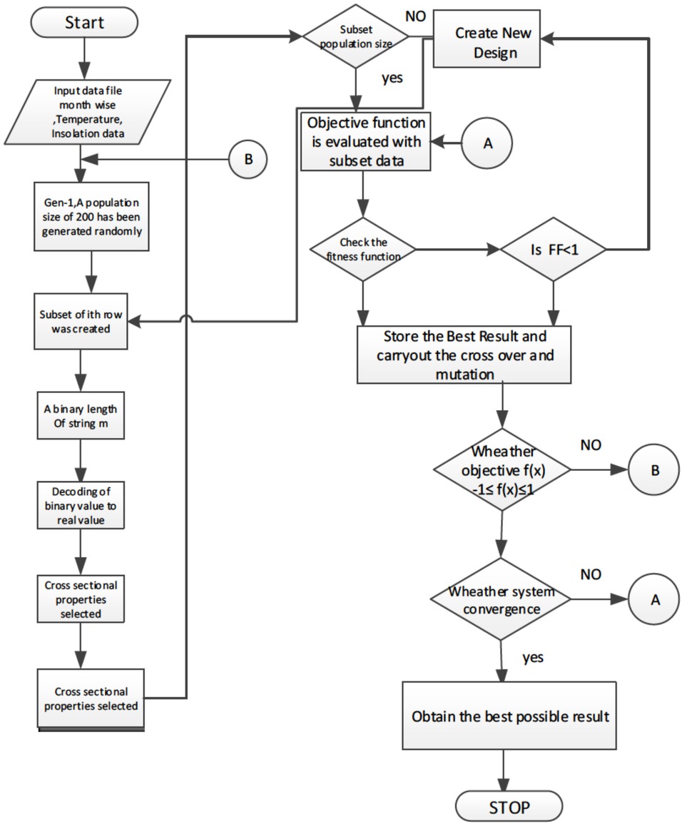
Algorithm of the Proposed GA Technique for Forecasting of Solar PV AC output

Table 1 shows the Observed and Calculated value of AC System Output along with the calculated system AC output Energy. Column 5 and 6 represents the Observed and calculated temperature using ANN of the Environment. In the present research Environmental temperature is considered to be the variable quantity which ultimately affects the performance of solar Photovoltaic system. Solar Irradiance for each month is assumed to be constant. The MSE and the Hidden layer details involved in the ANN model is shown in Table 2.

Table 1

Observed & Calculated value of Environmental Temperature and Solar PV Output

Month	Month	AC System Output(kWh)	AC System Output(kWh)-Calculated	Observed Temp.	Forecasted Temperature	Solar Radiation (kWh/m^2/day)
1	Jan	82257.875	81609.98438	26.53	26.77	4.2925396
2	Feb	100442.0313	99655.03125	30.97	30.91	5.67678547
3	Mar	135883.5938	134822.3594	34.81	37.95	6.68656969
4	Apr	142563.4375	141450.9688	39.92	40.28	6.84843159
5	May	145573.6094	144436.5625	39	40.23	6.48288298
6	Jun	125976.9844	124990.3047	32.34	37.9	5.53810167
7	Jul	119612.6172	118674.0938	31.28	32.85	4.99226809
8	Aug	114054.0469	113159.0781	32.68	35.56	4.94502401
9	Sep	113528.625	112638.5859	35.76	34.24	5.49704838
10	Oct	110454.2891	109588.3906	31.37	33.34	5.54661322
11	Nov	90045.02344	89337.64844	28.1	29.08	4.85409641
12	Dec	80529.05469	79894.44531	33.71	35.03	4.25716782

Table 2

MSE and the Hidden layer details

Number of Neurons			Mean Square Error
First Hidden Layer	Second Hidden Layer	Train	Validation	Test
10	10	0.0071	0.0198	0.0189
10	15	0.0082	0.0174	0.0192
10	20	0.0001	0.0146	0.0120
10	25	0.0009	0.0180	0.0173
10	30	0.0089	0.0191	0.0175
20	10	0.0023	0.0131	0.0117
20	15	0.0072	0.0171	0.0145
20	20	0.0018	0.0176	0.0169
20	25	0.0010	0.0195	0.0202
20	30	0.0017	0.0216	0.0185

From Table 2 it can be concluded that the for validation of 0.0131 the no. of hidden layer in the First part and Second part becomes 20 and 10 respectively. This confirms that for a test result of 0.0131, train was just only 0.0023. Hence the temperature corresponding to it was taken as the final calculated value or best value having the Error between the observed and forecasted value to be minimal.

Table 3 & 4 shows the Statistical Analysis such as Regression and Probability Analysis. From the Table 4 it can be found that the probability of prediction lies in the range of 12.5 to 95.833 percentile. The normal error present in the statistical analysis is of 1123.718. Now in order to validate the forecasting GA is applied for each month on the objective function as shown below

Table 3

Regression Statistics using ANOVA

ANOVA

	df	SS	MS	F	Significance F
Regression	1	3198110075	3198110075	14.78798	0.003236
Residual	10	2162641479	216264147.9
Total	11	5360751554

	Coefficients	Standard Error	t Stat	P-value	Lower 95.0%	Upper 95.0%
Intercept	−29300.6	37352.97934	−0.784425135	0.450973	−112528	53927.01
X Variable 1	4319.441	1123.241284	3.845514379	0.003236	1816.703	6822.178

Table 4

Probability Output Vs. Predicted Output

RESIDUAL OUTPUT			PROBABILITY OUTPUT

Observation	Predicted Y	Residuals	Percentile	Y
1	85294.14	−3036.265792	4.166667	80529.05
2	104472.5	−4030.425393	12.5	82257.88
3	121059.1	14824.48556	20.83333	90045.02
4	143131.4	−568.0116801	29.16667	100442
5	139157.6	6416.045461	37.5	110454.3
6	110390.1	15586.89424	45.83333	113528.6
7	105811.5	13801.13399	54.16667	114054
8	111858.7	2195.346965	62.5	119612.6
9	125162.6	−11633.95167	70.83333	125977
10	106200.2	4254.056217	79.16667	135883.6
11	92075.66	−2030.63895	87.5	142563.4
12	116307.7	−35778.66894	95.83333	145573.6

(14)y=3.6169x2+4077.3x−25301

The objective function as shown in equation 14 was derived from the Polynomialisation of Temperature and AC out put (kWh), which is shown in Figure 2

Figure 2

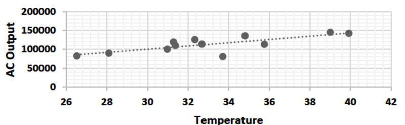
Polynomialisation of Temperature vs. AC Output Curve

Figure 3 shows the Simulation and data validation of Forecasted value with Genetic Algorithm. It is found that the Forecasted result as shown in the Table 1 is under the Normalcy. Similar to the AC Output Forecast, statistical analysis of Temperature is shown in the −5.

Figure 3

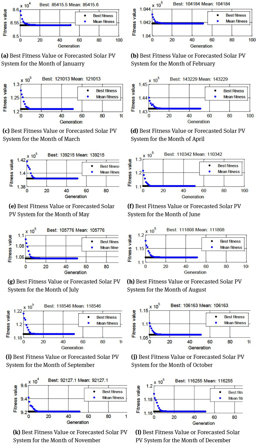
Shows the Best Fitness Value or Forecasted Solar PV System for the every month of Year

Table 5 and 6 shows the Statistical analysis of Temperature Histogram over 18 years and Regression analysis using ANOVA for Temperature respectively. The one-way analysis of variance (ANOVA) is used to determine whether there are any statistically significant differences between the means of two or more independent groups. Here df represents the degree of freedom which is 1 for Regression and 16 for Residual in this present study. Significance F represents the ratio of Mean Square Error to Sum Square Error, which is unity in the present case. This signifies that the forecasted result for solar PV is the best accurate one with respect to temperature. The F-test is used for comparing the factors of the total deviation. In the present analysis of ANOVA F is found to be 22.1812 which is inside the prescribed limit of F.

Table 5

Statistical Analysis of Temperature Histogram over 18 Years.

Sl. No.	Year	Average	RMSE	MAE/MAD	MAPE
1	2000	34.86091	1.977964	1.743796296	5%
2	2001	34.43364	1.606435	1.346018519	4%
3	2002	35.45273	2.282671	1.829259259	5%
4	2003	33.81273	0.583844	0.428703704	1%
5	2004	34.46455	1.285657	1.034259259	3%
6	2005	33.90273	0.986355	0.814259259	2%
7	2006	33.39909	1.636352	1.223425926	4%
8	2007	34.19818	1.124786	0.981666667	3%
9	2008	33.57364	1.361213	1.164351852	3%
10	2009	34.62818	1.244886	0.93537037	3%
11	2010	33.33455	1.791018	1.555277778	5%
12	2011	33.06	1.442175	0.97962963	3%
13	2012	32.68273	1.745693	1.461481481	4%
14	2013	32.63	1.279996	1.166944444	4%
15	2014	33.38091	1.11952	0.978518519	3%
16	2015	33.47727	0.854177	0.668333333	2%
17	2016	33.19364	1.66902	1.380092593	4%
18	2017	32.97818	1.398536	1.025925926	3%

Table 6

Regression Statistics using ANOVA for Temperature Analysis

ANOVA

	df	SS	MS	F	Significance F
Regression	1	6.166595666	6.166595666	23.18126642	1
Residual	16	4.256261451	0.266016341
Total	17	10.42285712

7 Conclusion

The level of solar Power that can be generated by a solar photovoltaic system depends upon the environment in which it is operated and two other important factor like the amount of solar insolation and temperature. Application of GA to Forecasting of the Solar AC output system is discussed in this paper. It is found that the forecasting using GA is much more convenient and accurate as compared to statistical method of analysis. In the next paper of this series Optimisation of Solar PV Output with respect to two variable such as Temperature as well as Solar Radiation will be presented. Grid connected solar Photovoltaic issues based on the Forecasted result and their mitigation techniques will be discussed in future work.

References

[1] B. Djurić, J. Kratica, D. Tošić, V. Filipović, Solving the maximally balanced connected partition problem in graphs by using genetic algorithm, Comput. Inform. 27(3), (2008), 341–354.Search in Google Scholar

[2] V. Filipović, J. Kratica, D. Tošić, I. Ljubić, Fine grained tournament selection for the simple plant location problem, in: Proceedings of the 5th Online World Conference on Soft Computing Methods in Industrial Applications – WSC5, 2000, 152–158.Search in Google Scholar

[3] D.R. Fulkerson, G. L. Nemhauser, L.E. Trotter, Two computationally diflcult set covering problems that arise in computing the l-width of incidence matrices of steiner triple systems, Math. Prog. Study 2 (1974), 72–81.10.1007/BFb0120689Search in Google Scholar

[4] M. Garey, D. Johnson, Computers and Intractability: a Guide to the Theory of NPcompleteness,Freeman, San Francisco 1979.Search in Google Scholar

[5] V. Guruswami, Inapproximability results for set splitting and satisfiability problems with no mixed clauses, Algorithmica 38 (2004), 451–469.10.1007/3-540-44436-X_16Search in Google Scholar

[6] J. Kratica, Improving performances of the genetic algorithm by caching, Comput. Artif. Intell.(1999), 271–283.Search in Google Scholar

[7] J. Kratica, V. Kovačević-Vujčić, M. Čangalović, Computing strong metric dimension of some special classes of graphs by genetic algorithms, Yugoslav. J. Oper. Res. 18(2) (2008), 43–51.10.2298/YJOR0802143KSearch in Google Scholar

[8] J. Kratica, M. Čangalović, V. Kovačević-Vujčić, Computing minimal doubly resolving sets of graphs, Comput. Oper. Res. 36(7) (2009), 2149–2159.10.1016/j.cor.2008.08.002Search in Google Scholar

[9] J. Kratica, V. Kovačević-Vujčić, M. Čangalović, Computing the metric dimension of graphs by genetic algorithms, Comput. Optim. Appl. 44(2) (2009), 343–361.10.1007/s10589-007-9154-5Search in Google Scholar

[10] R. H. Kwon, G. V. Dalakouras, C. Wang, On a posterior evaluation of a simple greedy method for set packing, Optim. Lett. 2 (2008), 587–597.10.1007/s11590-008-0085-6Search in Google Scholar

[11] L. Liberti, N. Maculan, Y. Zhang, Optimal configuration of gamma raymachine radiosurgery units: the sphere covering subproblem, Optim. Lett. 3(2009), 109–121.10.1007/s11590-008-0095-4Search in Google Scholar

[12] M. Mitchell, An Introduction to Genetic Algorithms, MIT Press, Cambridge, Massachusetts, 1999.Search in Google Scholar

[13] Paszynska, M. Paszynski, Application of a hierarchical chromosome based genetic algorithm to the problem of finding optimal initial meshes for the self-adaptive hp-FEM, Comput. Inform. 28(2) (2009), 209–223.Search in Google Scholar

[14] Z. Stanimirović, J. Kratica, Dj. Dugošija, Genetic algorithms for solving the discrete ordered median problem, Eur. J. Oper. Res. 182(3) (2007), 983–1001.10.1016/j.ejor.2006.09.069Search in Google Scholar

[15] C.Wang, M. T. Thai, Y. Li, F.Wang,W.Wu, Optimization scheme for sensor coverage scheduling with bandwidth constraints, Optim. Lett. 3 (2009), 63–75.10.1007/s11590-008-0091-8Search in Google Scholar

[16] B. Yuan, M. Orlowska, S. Sadiq, Extending a class of continuous estimation of distribution algorithms to dynamic problems, Optim. Lett. 2(2008), 433–443.10.1007/s11590-007-0071-4Search in Google Scholar

[17] J. Zhang, Y. Ye, Q. Han, Improved approximations for max set splitting and max NAE SAT, Discrete Appl. Math. 142(2004), 133–149.10.1016/j.dam.2002.07.001Search in Google Scholar

[18] SPE, 2017. SPE, (Solar Power Europe) global market outlook for solar power 2017–2021; 2017<http://www.solarpowereurope.org/insights/global-marketoutllook/>Search in Google Scholar

[19] Kaur A, Nonnenmacher L, Pedro HTC, Coimbra CFM. Benefits of solar forecasting for energy imbalance markets. Renew Energy 2016;86:819–30. http://dx.doi.org/10.1016/j.renene 2015.09.011.10.1016/j.renene.2015.09.011Search in Google Scholar

[20] Van der Kam M, Van Sark WGJHM. Smart charging of electric vehicles with photovoltaic power and vehicle-to-grid technology in the residential sector: a case study. Appl Energy 2015;152:20–30.10.1016/j.apenergy.2015.04.092Search in Google Scholar

[21] Verbong GP, Beemsterboer S, Sengers F. Smart grids or smart users? Involving users in developing a low carbon electricity economy. Energy Policy 2013;52:117–25. http://dx.doi.org/10.1016/j.enpol.2012.05.00310.1016/j.enpol.2012.05.003Search in Google Scholar

[22] Castillo-Cagigal M, Caamano-Martín E, Matallanas E, Masa-Bote D, Gutiérrez A, Monasterio-Huelin F, et al. PV self-consumption optimization with storage and active DSM for the residential sector. Solar Energy 2011;85(9):2338–48. http://dx.doi.org/10.1016/j.solener.2011.06.02810.1016/j.solener.2011.06.028Search in Google Scholar

[23] Matallanas E, Castillo-Cagigal M, Gutiérrez A, Monasterio-Huelin F, Caamaño- Martín E, Masa D, et al. Neural network controller for active demand-side management with PV energy in the residential sector. Appl Energy 2012;91(1):90–7. http://dx.doi.org/10.1016/j.apenergy.2011.09.00410.1016/j.apenergy.2011.09.004Search in Google Scholar

[24] Bird L, Lew D, Milligan M, Carlini EM, Estanqueiro A, Flynn D, et al. Wind and solar energy curtailment: a review of international experience. Renew Sustain Energy Rev 2016;65:577–86. http://dx.doi.org/10.1016/j.rser.2016.06.08210.1016/j.rser.2016.06.082Search in Google Scholar

[25] Litjens GBMA, Worrell E, Van Sark WGJHM. Influence of demand patterns on the optimal orientation of photovoltaic systems. Solar Energy 2017;155:1002–14. http://dx.doi.org/10.1016/j.solener.2017.07.00610.1016/j.solener.2017.07.006Search in Google Scholar

[26] 3E. Meta PV - cost-effective integration of Photovoltaics in distribution grids: results and recommendations; 2015<http://www.metapv.eu/finalreport>Search in Google Scholar

[27] Staats M, de Boer-Meulman P, van Sark W. Experimental determination of demand side management potential of wet appliances in the Netherlands. Sustain Energy, Grids Netw 2017;9:80–94<http://www.sciencedirect.com/science/article/pii/S2352467716302144>10.1016/j.segan.2016.12.004Search in Google Scholar

[28] Fang X, Misra S, Xue G, Yang D.Smart grid - the new and improved power grid: a survey. IEEE Commun Surv Tut 2012;14(4):944–80.10.1109/SURV.2011.101911.00087Search in Google Scholar

[29] la Parra ID, Marcos J, García M, Marroyo L. Storage requirements for PV power ramp-rate control in a PV fleet. Solar Energy 2015;118:426–40<http://www.sciencedirect.com/science/article/pii/S0038092X15003102>10.1016/j.solener.2015.05.046Search in Google Scholar

[30] DNV-GL, 2015. Power matching city phase II report by DNV-GL http://www.powermatchingcity.nl/; 2015http://www.powermatchingcity.nl/data/docs/PowerMatching%20City_brochure_final_UK_29-04-2015_lowres.pdfSearch in Google Scholar

[31] Mwasilu F, Justo JJ, Kim E-K, Do TD, Jung J-W. Electric vehicles and smart grid interaction: a review on vehicle to grid and renewable energy sources integration. Renew Sustain Energy Rev 2014;34:501–16. http://dx.doi.org/10.1016/j.rser 2014.03.031.10.1016/j.rser.2014.03.031Search in Google Scholar

[32] Lorenz E, Heinemann D. Earth and planetary sciences, chapter 1.13. Prediction of solar irradiance and photovoltaic power. Elsevier Ltd.; 2012. p. 239–92. http://dx.doi.org/10.1016/B978-0-08-087872-0.00114-1.ISBN978008087873710.1016/B978-0-08-087872-0.00114-1Search in Google Scholar

[33] Diagne M, David M, Lauret P, Boland J, Schmutz N. Review of solar irradiance forecasting methods and a proposition for small-scale insular grids. Renew Sustain Energy Rev 2013;27:65–76. http://dx.doi.org/10.1016/j.rser.2013.06.04210.1016/j.rser.2013.06.042Search in Google Scholar

[34] Kleissl J, editor. Solar energy forecasting and resource assessment. Oxford UK: Elsevier Academic Press; 2013. ISBN 9780123971777.Search in Google Scholar

[35] Redmund J, Calhau C, Perret L, Marcel D. Characterization of the spatio-temporal variations and ramp rates of solar radiation and PV - Report of IEA Task 14 Subtask 1.3. Tech. Rep. IEA PVPS T14-05:2015, International Energy Agency – Photovoltaic Power Systems Programme; 2015.Search in Google Scholar

[36] Antonanzas J, Osorio N, Escobar R, Urraca R, Martinez-de pison FJ, Antonanzastorres F. Review of photovoltaic power forecasting. Solar Energy 2016;136:78–111. http://dx.doi.org/10.1016/j.solener.2016.06.06910.1016/j.solener.2016.06.069Search in Google Scholar

[37] Hammer A, Heinemann D, Lorenz E, Lückehe B. Short-term forecasting of solar radiation: a statistical approach using satellite data. Solar Energy 1999;67(1):139–50. http://dx.doi.org/10.1016/S0038-092X(00)00038-410.1016/S0038-092X(00)00038-4Search in Google Scholar

[38] Pelland S, Galanis G, Kallos G. Solar and photovoltaic forecasting through postprocessing of the global environmental multiscale numerical weather prediction model. Prog Photovolt: Res Appl 2013;21(3):284–96. http://dx.doi.org/10.1002/pip.118010.1002/pip.1180Search in Google Scholar

[39] Mathiesen P, Collier C, Kleissl J. A high-resolution, cloud-assimilating numerical weather prediction model for solar irradiance forecasting. Solar Energy 2013;92:47–61. http://dx.doi.org/10.1016/j.solener.2013.02.01810.1016/j.solener.2013.02.018Search in Google Scholar

[40] Mathiesen P, Kleissl J. Evaluation of numerical weather prediction for intra-day solar forecasting in the continental united states. Solar Energy 2011;85(5):967–77. http://dx.doi.org/10.1016/j.solener.2011.02.01310.1016/j.solener.2011.02.013Search in Google Scholar

[41] Perez R, Kivalov S, Schlemmer J, Hemker Jr. K, Renné D, Hoff T. Validation of short and medium term operational solar radiation forecasts in the {US}. Solar Energy 2010;84(12):2161–72. http://dx.doi.org/10.1016/j.solener.2010.08.01410.1016/j.solener.2010.08.014Search in Google Scholar

[42] Marquez R, Coimbra CFM. Intra-hour DNI forecasting based on cloud tracking image analysis. Solar Energy 2013;91:327–36. http://dx.doi.org/10.1016/j.solener.2012.09.01810.1016/j.solener.2012.09.018Search in Google Scholar

[43] Chow CW, Urquhart B, Lave M, Dominguez A, Kleissl J, Shields J, et al. Intra-hour forecasting with a total sky imager at the UC San Diego solar energy testbed. Solar Energy 2011;85(11):2881–93. http://dx.doi.org/10.1016/j.solener.2011.08.02510.1016/j.solener.2011.08.025Search in Google Scholar

[44] Chow CW, Belongie S, Kleissl J. Cloud motion and stability estimation for intra-hour solar forecasting. Solar Energy 2015;115:645–55http://www.sciencedirect.com/science/article/pii/S0038092X1500156510.1016/j.solener.2015.03.030Search in Google Scholar

[45] Chu Y, Pedro HTC, Coimbra CFM. Hybrid intra-hour DNI forecasts with sky image processing enhanced by stochastic learning. Solar Energy 2013;98:592–603 http://linkinghub.elsevier.com/retrieve/pii/S0038092X1300432510.1016/j.solener.2013.10.020Search in Google Scholar

[46] Chu Y, Pedro HTC, Li M, Coimbra CFM. Real-time forecasting of solar irradiance ramps with smart image processing. Solar Energy 2015;114:91–104 http://linkinghub.elsevier.com/retrieve/pii/S0038092X1500038910.1016/j.solener.2015.01.024Search in Google Scholar

[47] Peng Z, Yu D, Huang D, Heiser J, Yoo S, Kalb P. 3D cloud detection and tracking system for solar forecast using multiple sky imagers. Solar Energy 2015;118(August):496–519. http://dx.doi.org/10.1016/j.solener.2015.05.03710.1016/j.solener.2015.05.037Search in Google Scholar

[48] Muselli M, Poggi P, Notton G, Louche A. First order markov chain model for generating synthetic “typical days” series of global irradiation in order to design photovoltaic stand alone systems. Energy Convers Manage 2001;42(6):675–87. http://dx.doi.org/10.1016/S0196-8904(00)00090-X10.1016/S0196-8904(00)00090-XSearch in Google Scholar

[49] Li Y-Z, Luan R, Niu J-c. Forecast of power generation for grid-connected photovoltaic system based on grey model and markov chain. 3rd IEEE conference on industrial electronics and applications, 2008, ICIEA 2008 IEEE; 2008. p. 1729–33. http://dx.doi.org/10.1109/ICIEA.2008.458281610.1109/ICIEA.2008.4582816Search in Google Scholar

[50] Duda, Hart. Pattern classification. 2nd ed. New York: John Wiley & Sons; 2000.Search in Google Scholar

[51] Yakowitz S. Nearest-neighbour methods for time series analysis. J Time Ser Anal 1987;8(2):235–47. http://dx.doi.org/10.1111/j.1467-9892.1987.tb00435.x10.1111/j.1467-9892.1987.tb00435.xSearch in Google Scholar

[52] Reikard G. Predicting solar radiation at high resolutions: a comparison of time series forecasts. Solar Energy 2009;83(3):342–9http://linkinghub.elsevier.com/retrieve/pii/S0038092X0800210710.1016/j.solener.2008.08.007Search in Google Scholar

[53] Bacher P, Madsen H, Nielsen HA. Online short-term solar power forecasting. Solar Energy 2009;83(10):1772–83. http://dx.doi.org/10.1016/j.solener.2009.05.01610.1016/j.solener.2009.05.016Search in Google Scholar

[54] Yang D, Sharma V, Ye Z, Lim LI, Zhao L, Aryaputera AW. Forecasting of global horizontal irradiance by exponential smoothing, using decompositions. Energy 2015;81:111–9http://linkinghub.elsevier.com/retrieve/pii/S036054421401352810.1016/j.energy.2014.11.082Search in Google Scholar

[55] Hyndman R, Koehler AB, Ord JK, Snyder RD. Forecasting with exponential smoothing: the state space approach. Springer Science & Business Media; 2008.10.1007/978-3-540-71918-2Search in Google Scholar

[56] Urraca R, Antonanzas J. Smart baseline models for solar irradiation forecasting Spanish agency for irrigation in agriculture. Energy Convers Manage 2016;108:539–48. http://dx.doi.org/10.1016/j.enconman.2015.11.03310.1016/j.enconman.2015.11.033Search in Google Scholar

[57] Sfetsos A, Coonick A. Univariate and multivariate forecasting of hourly solar radiation with artificial intelligence techniques. Solar Energy 2000;68(2):169–78. http://dx.doi.org/10.1016/S0038-092X(99)00064-X10.1016/S0038-092X(99)00064-XSearch in Google Scholar

[58] Voyant C, Muselli M, Paoli C, Nivet M-L. Optimization of an artificial neural network dedicated to the multivariate forecasting of daily global radiation. Energy 2011;36(1):348–59. http://dx.doi.org/10.1016/j.energy.2010.10.03210.1016/j.energy.2010.10.032Search in Google Scholar

[59] Pedro HTC, Coimbra CFM. Assessment of forecasting techniques for solar power production with no exogenous inputs. Solar Energy 2012;86(7):2017–28.http://dx.doi.org/10.1016/j.solener.2012.04.00410.1016/j.solener.2012.04.004Search in Google Scholar

[60] Fonecsa Jr. JG, Oozeki T, Takashima T, Koshimizu G, Uchida Y, Ogimoto K. Use of support vector regression and numerically predicted cloudiness to forecast power output of a photovoltaic power plant in Kitakyushu, Japan. Prog Photovolt: Res Appl 2012;20:874–82. http://dx.doi.org/10.1002/pip.115210.1002/pip.1152Search in Google Scholar

[61] Boland J. Spatial-temporal forecasting of solar radiation. Renew Energy 2015;75:607–16. http://dx.doi.org/10.1016/j.renene.2014.10.03510.1016/j.renene.2014.10.035Search in Google Scholar

[62] Rana M, Koprinska I, Agelidis VG. Univariate and multivariate methods for very short-term solar photovoltaic power forecasting. Energy Convers Manage 2016;121:380–90. http://dx.doi.org/10.1016/j.enconman.2016.05.02510.1016/j.enconman.2016.05.025Search in Google Scholar

[63] Dambreville R, Blanc P, Chanussot J, Boldo D, Dubost S. Very short term forecasting of the global horizontal irradiance through Helioclim maps. IREC 2014:291–300. http://dx.doi.org/10.1016/j.renene.2014.07.01210.1109/IREC.2014.6826905Search in Google Scholar

[64] Zagouras A, Pedro HTC, Coimbra CFM. On the role of lagged exogenous variables and spatio-temporal correlations in improving the accuracy of solar forecasting methods. Renew Energy 2015;78:203–18. http://dx.doi.org/10.1016/j.renene.2014.12.07110.1016/j.renene.2014.12.071Search in Google Scholar

[65] Wolff B, Kühnert J, Lorenz E, Kramer O, Heinemann D. Comparing support vector regression for PV power forecasting to a physical modeling approach using measurement, numerical weather prediction, and cloud motion data. Solar Energy 2016;135:197–208.10.1016/j.solener.2016.05.051Search in Google Scholar

[66] Vaz AGR, Elsinga B, Van Sark WGJHM, Brito MC. An artificial neural network to assess the impact of neighbouring photo-voltaic systems in power forecasting in Utrecht, the Netherlands. Renew Energy 2016;85:631–41http://linkinghub.elsevier.com/retrieve/pii/S096014811530084710.1016/j.renene.2015.06.061Search in Google Scholar

[67] Inman RH, Pedro HTC, Coimbra CFM. Solar forecasting methods for renewable energy integration. Prog Energy Combust Sci 2013;39(6):535–76. http://dx.doi.org/10.1016/j.pecs.2013.06.00210.1016/j.pecs.2013.06.002Search in Google Scholar

[68] Widén J, Carpman N, Castellucci V, Lingfors D, Olauson J, Remouit F, et al. Variability assessment and forecasting of renewables: a review for solar, wind, wave and tidal resources. Renew Sustain Energy Rev 2015;44:356–75. http://dx.doi.org/10.1016/j.rser.2014.12.01910.1016/j.rser.2014.12.019Search in Google Scholar

[69] Barbieri F, Rajakaruna S, Ghosh A. Very short-term photovoltaic power forecasting with cloud modeling: a review. Renew Sustain Energy Rev 2017;75(August 2015):242–63. http://dx.doi.org/10.1016/j.rser.2016.10.06810.1016/j.rser.2016.10.068Search in Google Scholar

[70] Mellit A, Kalogirou Sa. Artificial intelligence techniques for photovoltaic applications: a review. Prog Energy Combust Sci 2008;34(5):574–632. http://dx.doi.org/10.1016/j.pecs.2008.01.00110.1016/j.pecs.2008.01.001Search in Google Scholar

[71] Voyant C, Notton G, Kalogirou S, Nivet ML, Paoli C, Motte F, et al. Machine learning methods for solar radiation forecasting: a review. Renew Energy 2017;105:569–82. http://dx.doi.org/10.1016/j.renene.2016.12.09510.1016/j.renene.2016.12.095Search in Google Scholar

[72] Murata A, Otani K. An analysis of time-dependent spatial distribution of output power from very many PV power systems installed on a nation-wide scale in Japan. Solar Energy Materials Solar Cells 1997;47(1–4):197–202. http://dx.doi.org/10.1016/S0140-6701(97)82039-510.1016/S0927-0248(97)00040-8Search in Google Scholar

[73] Wiemken E, Beyer H, Heydenreich W, Kiefer K. Power characteristics of PV ensembles: experiences from the combined power production of 100 grid connected PV systems distributed over the area of Germany. Solar Energy 2001;70(6):513–8. http://dx.doi.org/10.1016/S0038-092X(00)00146-810.1016/S0038-092X(00)00146-8Search in Google Scholar

[74] Perez R, Kivalov S, Schlemmer J, Hemker K, Hoff TE. Short-term irradiance variability: preliminary estimation of station pair correlation as a function of distance. Solar Energy 2012;86(8):2170–6. http://dx.doi.org/10.1016/j.solener.2012.02.02710.1016/j.solener.2012.02.027Search in Google Scholar

[75] Hoff TE, Perez R. Modeling PV fleet output variability. Solar Energy 2012;86(8):2177–89. http://dx.doi.org/10.1016/j.solener.2011.11.00510.1016/j.solener.2011.11.005Search in Google Scholar

[76] Perez MJR, Fthenakis VM. On the spatial decorrelation of stochastic solar resource variability at long timescales. Solar Energy 2015;117:46–58. http://dx.doi.org/10.1016/j.solener.2015.04.02010.1016/j.solener.2015.04.020Search in Google Scholar

[77] Lave M, Kleissl J, Arias-Castro E. High-frequency irradiance fluctuations and geographic smoothing. Solar Energy 2012;86(8):2190–9http://linkinghub.elsevier.com/retrieve/pii/S0038092X1100261110.1016/j.solener.2011.06.031Search in Google Scholar

[78] Hinkelman LM. Differences between along-wind and crosswind solar irradiance variability on small spatial scales. Solar Energy 2013;88:192–203. http://dx.doi.org/10.1016/j.solener.2012.11.01110.1016/j.solener.2012.11.011Search in Google Scholar

[79] Perpiñán O, Marcos J, Lorenzo E. Electrical power fluctuations in a network of DC/AC inverters in a large PV plant: relationship between correlation, distance and time scale. Solar Energy 2013;88:227–41.10.1016/j.solener.2012.12.004Search in Google Scholar

[80] Elsinga B, Van Sark WGJHM. Spatial power fluctuation correlations in urban rooftop photovoltaic systems. Prog Photovolt: Res Appl 2015;23(10):1390–7. http://dx.doi.org/10.1002/pip.253910.1002/pip.2539Search in Google Scholar

[81] Lohmann GM, Monahan AH, Heinemann D. Local short-term variability in solar irradiance. Atmos Chem Phys 2016;16(10):6365–79. http://dx.doi.org/10.5194/acp-16-6365-201610.5194/acp-16-6365-2016Search in Google Scholar

[82] Elsinga B, Van Sark WGJHM. Inter-system time lag due to clouds in an urban PV ensemble. In: Conference record of the IEEE photovoltaic specialists conference; 2014. p. 754–8.10.1109/PVSC.2014.6925029Search in Google Scholar

[83] Lonij VP, Brooks AE, Cronin AD, Leuthold M, Koch K. Intra-hour forecasts of solar power production using measurements from a network of irradiance sensors. Solar Energy 2013;97:58–66. http://dx.doi.org/10.1016/j.solener.2013.08.00210.1016/j.solener.2013.08.002Search in Google Scholar

Received: 2019-07-19

Accepted: 2020-04-29

Published Online: 2020-07-07

This work is licensed under the Creative Commons Attribution 4.0 International License.

Articles in the same Issue

https://doi.org/10.1515/eng-2020-0073

Keywords for this article

Solar PV; Maximum Power Point Tracking; AI-Techniques; Forecasting

Creative Commons

BY 4.0