Disjoint Sum of Products by Orthogonalizing Difference-Building ⴱ
-
Yavuz Can
 ,
Önder Yaz
,
Önder Yaz

Abstract
The orthogonalization of Boolean functions in disjunctive form, that means a Boolean function formed by sum of products, is a classical problem in the Boolean algebra. In this work, the novel methodology ORTH[ⴱ] of orthogonalization which is an universally valid formula based on the combination technique »orthogonalizing difference-building ⴱ« is presented. Therefore, the technique ⴱ is used to transform Sum of Products into disjoint Sum of Products. The scope of orthogonalization will be solved by a novel formula in a mathematically easier way. By a further procedure step of sorting product terms, a minimized disjoint Sum of Products can be reached. Compared to other methods or heuristics ORTH[ⴱ] provides a faster computation time.
1 Introduction and Preliminaries
A Boolean function of n variables is defined as the mapping f (x) : {0, 1}n → {0, 1}. Four normal forms of Boolean functions exist, the disjunctive normal form (DNF), conjunctive normal form (CNF), antivalence normal form (ANF) and equivalence normal form (ENF), which consist of either product terms
A is the index set of the running index i. The AF is a special form of Exclusive-Or Sum of Products (ESOP) and is defined as
The orthogonality of a Boolean functions is a special attribute. A function is orthogonal if their terms have the characteristic of being disjoint in pairs in at least one variable. Thus, the following applies for the disjoint Sum of Products (dSOP):
An orthogonal representation of a SOP, that means dSOP, is characterized by product terms which are disjoint to one another in pairs [3, 4]. Consequently, the intersection of these product terms results in 0. The orthogonal representation of a DF - disjoint Sum of Products - is equal to the orthogonal form of an AF - the disjoint Exclusive-Or Sum of Products. In this case, it applies dSOP(x) = dESOP(x) [3, 4, 5]. That means, the dSOP is equivalent to dESOP consisting of the same product terms and differ only in the logical connectivity between the product terms. This relationship can be explained well with the following definition out of [6], if both product terms pi(x) and pj(x) are disjoint to each other. A SOP of two product terms can be transformed into an ESOP by:
In the special case, that both products terms are disjoint, building their conjunction results to 0. As xi ⊕ 0 = xi is, following relation follows from the Eq. (4):
In this case, the left side is equal to the right side which means that a dSOP is equivalent to a dESOP. It applies dSOP(x) = dESOP(x).
In a K-map a dSOP is characterized by non-overlapping cubes (Figure 1). Special calculations can be easier solved in another form. It simplifies the handling of further calculations in applications of electrical engineering, e.g. calculation of suitable test patterns for combinational circuits for verifying feasible logical faults, which can mathematically be determined by Boolean Differential Calculus (BDC) [1, 7]. That means, the orthogonalization of a SOP facilitates the transformation into an equivalent dESOP [1, 3, 8] and this characteristic simplifies the handling of BDC especially in Ternary-Vector-List (TVL) arithmetic [3, 9, 10, 11]. Due to the restricted number of variables the terms of SOP are not priory disjoint. However, the disjoint form can be calculated by using a novel Boolean formula based on the novel combining technique of »orthogonalizing difference-building ⴱ«.

Difference between SOP and dSOP in a K-map
2 Method of Orthogonalization
2.1 Orthogonalizing Difference-Building ⴱ
Orthogonalizing difference-building ⴱ is the composition of two calculation steps - the usual difference-building out of the set theory and the subsequent orthogonalization, as shown in Figure 2. The result of ⴱ is orthogonal in contrast to the result out of the method difference-building. Both results are different in their representations but homogenous in their covering of 1s. They only differ in their form of coverage, whereas the method ⴱ constitutes the solution in already orthogonal form. This method ⴱ is generally valid and equivalent to the usual method of difference-building [3]. The orthogonalizing difference-building ⴱ corresponds to the removal of the intersection which is formed between the minuend product
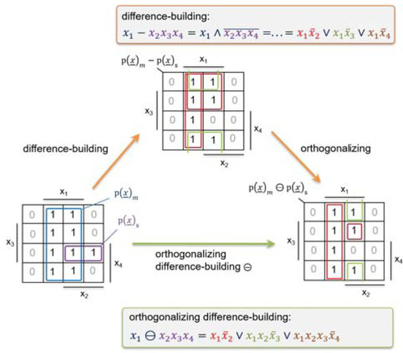
ⴱ: Two procedures in one step
Example 1: A subtrahend
The explanation of Eq. (6) is given by the following points:
The first literal of the subtrahend, here x2, is taken complementary and build the intersection with the minuend, here x1. Consequently, the first term of the difference is x1x2.
Then the second literal, here x3, is taken complementary and the intersection with the minuend and the first literal x2 of the subtrahend is built. Therefore, the second term is x1x2x3.
Following the next literal, here x4, is taken complementary and the intersection with the minuend and the first literal x2 and second literal x3 of the subtrahend is built. Thus, the third term of the difference is x1x2x3x4.
This process is continued until all literals of the subtrahend are singly complemented and linked by building the intersection with the minuend in a separate term.
north as the number of product terms in the orthogonal result corresponds to the number of literals presented in the subtrahend ps(x) and are not presented in the minuend
If the subtrahend is already orthogonal to the minuend
(7)The difference between 0 and the subtrahend is the subtrahend itself:
(8)The result between 1 and subtrahend is the complement of the subtrahend which results in a dSOP:
(9)Thereby, the subset symbol ⊆ of the set theory is transferred to switching algebra. The result between subtrahend and minuend is empty if the subtrahend is already completely contained in the minuend. If the subtrahend is the subset of the minuend
2.2 Orthogonalization of SOP
2.2.1 Mathematical Methodology
The orthogonalization of every SOP(x) consisting of at least two product terms (N > 1) can be performed by Eq. (11) which bases on the Eq. (6), which is based on the combination technique of ⴱ [3]. The order of the calculation is important. That means, the first two product terms must be calculated and then the third product term must be calculated with the result of the two product terms before, and so on. The result of
Example 2: Function
Function
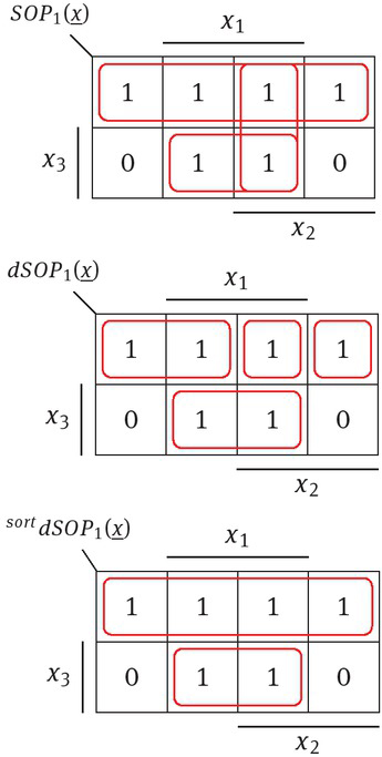
Comparison of SOP1(⨱), dSOP1(⨱) and sortdSOP1(⨱)
Example 3: Now, the sorted function
Function
2.2.2 Algorithm
The corresponding Algorithm ORTH[ⴱ], whose pseudo code is shon in the Table 1 outlines the computational procedure of orthogonalization of a SOP according to the formula in Eq. (11). To obtain dSOP with fewer number of product terms, the sub-functions absorb() and sort() are additionally used. absorb() is a function which reduces the number of product terms of the SOP, which serves as the input of the algorithm. The reduction is achieved by by absorption of smaller product terms, which consists of higher number of variables, by larger product terms, which consists of lower number of variables if those are already covered by the larger ones (following example):
Pseudo-Code of the Algorithm ORTH[ⴱ]
| functiondSOP(SOP) |
| SOP.absorb() |
| SOP.sort() |
| for z=0 to N do () |
| tmpSOP.add_pipi.get_p(z) |
| for i=z+1 to N do () |
| tmpSOP.ⴱtmpSOP, pi.get_p(i) |
| dSOP.add(tmpSOP) |
| return dSOP |
The product term x1 is absorbing the other two product term. Additionally, absorb() reduces duplicated product terms to a single term which is demonstrated with the following example:
Consequently, by using absorb() the number of product terms, that have to be treated decreases. With the optionally function sort() follows the resorting of the product terms from smaller product terms to larger product terms. After proceeding these two sub-functions absorb() and sort() the process of orthogonalization ORTH[ⴱ] according to the method ⴱ is performed.
3 Comparison and Measurement
3.1 North before and after Sorting
However, to make a statement about the optimized form, the optimum minimization would have to be defined, which has not yet been clarified. Table 2 illustrates the percentage of reduced terms by the use of subsequent procedure of sorting. The procedure of sorting brings an advantage for gaining minimized dSOP. Firstly, a list of ten non-orthogonal functions in respect to N = {5, 10, 15} and dimension xn = {5, 6, . . . , 50} were created. Consequently, per each N has produced 50 different non-orthogonal SOPs. Subsequently, each SOP was orthogonalized according to the method ⴱ before and after sorting. The resulting number of product terms North in dSOP and sortNorth in sortdSOP in respect to N and xn were determined (Figure 4) and compared. The number of product terms of a sorted SOP is fewer then the unsorted SOP. It follows sortNorth(N, xn) < North(N, xn). An average value of these values was calculated for each dimension xn. Thereby, the results of the quotients of the average number of disjoint product terms were obtained. Furthermore, quotients of North and sortNorth in percentage value were gained. The minus signifies that in that case the number of North is fewer. Finally, a total average percentage value per each N was determined out of these average values (Table 2). Three in their number. Consequently, an additional procedure of sorting leads to a dSOP with fewer number of product terms. Minimalization of approximately 17% till 28% is obtained in comparison to a dSOP which has not been sorted before.

Average number of North and sortNorth
Percentage Value of
| Percentage Value [%] | |||
|---|---|---|---|
| xn | |||
| 5 | 0.0 | 8.6 | - |
| 6 | 23.6 | 29.0 | - |
| 7 | 28.8 | 11.8 | 24.6 |
| 8 | 30.2 | 27.0 | 28.7 |
| 9 | 73.3 | 52.0 | 32.8 |
| 10 | 6.1 | 24.6 | 29.6 |
| 28 | 13.6 | 10.5 | 40.9 |
| 29 | 2.7 | 58.6 | 22.3 |
| 30 | 38.6 | 25.8 | 50.6 |
| 31 | 17.8 | 8.5 | 18.0 |
| 45 | −1.6 | 9.4 | −2.8 |
| 46 | −5.4 | 6.5 | 13.1 |
| 47 | 14.8 | 0.6 | 38.4 |
| 48 | 8.8 | 20.2 | 16.4 |
| 49 | 1.2 | −13.1 | 18.6 |
| 50 | −2.5 | 30.6 | 8.8 |
| ∅ | 17.3 | 21.7 | 27.6 |
3.2 Comparison in Number of Terms North
The number of the disjoint product terms North in a dSOP produced by ORTH[ⴱ] is analyzed in comparison to the heuristic ORTH[DSOP] in [5], the method ORTH[m1] in [12] and a varied form of ORTH[DSOP] as ORTH[DSOP2]. In the varied form ORTH[DSOP2] the minimization function “espresso.exe” was replaced by absorb(). The comparisions in respect to N = {2, 5, 10, 15, 20, 25} and xn = {1, 2, . . . , 50} are shown in Figure 5. The corresponding average values
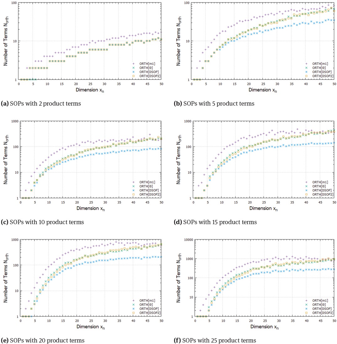
Average number of the North in the dSOP
Average of the number of terms North and relation to ORTH[ⴱ]
| xn | |||||||
|---|---|---|---|---|---|---|---|
| 2 | 6,22 | 6,30 | 6,30 | 9,45 | 1,01 | 1,01 | 1,52 |
| 5 | 29,52 | 18,57 | 29,11 | 43,22 | 0,63 | 0,99 | 1,46 |
| 10 | 86,72 | 44,96 | 88,32 | 127,35 | 0,52 | 1,02 | 1,47 |
| 15 | 164,05 | 77,82 | 165,90 | 249,31 | 0,47 | 1,01 | 1,52 |
| 20 | 248,18 | 115,97 | 258,58 | 431,67 | 0,47 | 1,04 | 1,74 |
| 25 | 369,09 | 162,79 | 393,47 | 650,57 | 0,44 | 1,07 | 1,76 |
| ∅ | 150,63 | 71,07 | 156,95 | 251,93 | 0,47 | 1,04 | 1,67 |
3.3 Comparison in Computation Time
In this section the comparison of all four approaches relating to the computation time in respect to N = {2, 5, 10, 15, 20, 25} and xn = {1, 2, . . . , 50} as shown in the Figures 6a) - f) is given. The corresponding average values of the calculation times and the ratios to the method ORTH[ⴱ] are given in the Table 4. The computation times of method ORTH[ⴱ] is faster in comparison to the heuristic ORTH[DSOP], ORTH[m1] and the varied form ORTH[DSOP2]. The complexity class of ORTH[ⴱ] totals up to Θ(n5). The distinction is that the noval method ORTH[ⴱ] calculates the orthogonalizing difference-building ⴱ consistently no matter if two product terms are orthogonal or not. As this consideration takes place in method ORTH[m1] in [1], the computation time is likely to be deteriorated. Thus unnecessary calculations are not to be carried out in the method ORTH[ⴱ]. By the use of “espresso.exe” in ORTH[DSOP] the procedure time of orthogonalization is more slowly. This is also confirmed by replacing the function with absorb(), which is shown by the charts of ORTH[DSOP2]. Therefore, its computation time is decelerated. Due to the replacement of the minimization function by absorb() in ORTH[DSOP2] the calculation time gets faster in comparison to ORTH[DSOP]. However, it is still higher than the computation time of the novel method ORTH[ⴱ]. In summary, it has to be clarified here that the new method has faster computation time than the other approaches. ORTH[ⴱ] is approximately 1000 times faster in comparison to ORTH[DSOP], approximately 25 times faster than ORTH[DSOP2] and twice as fast than ORTH[m1]. Even if the two sub-functions absorb() and sort() are excluded, the method ORTH[ⴱ] provides computation time, which are reduced, as shown in Figure 6a) - f). The measurements are limited to the dimension xn = 50. Against this, for dimension xn > 50 similar results are expected.
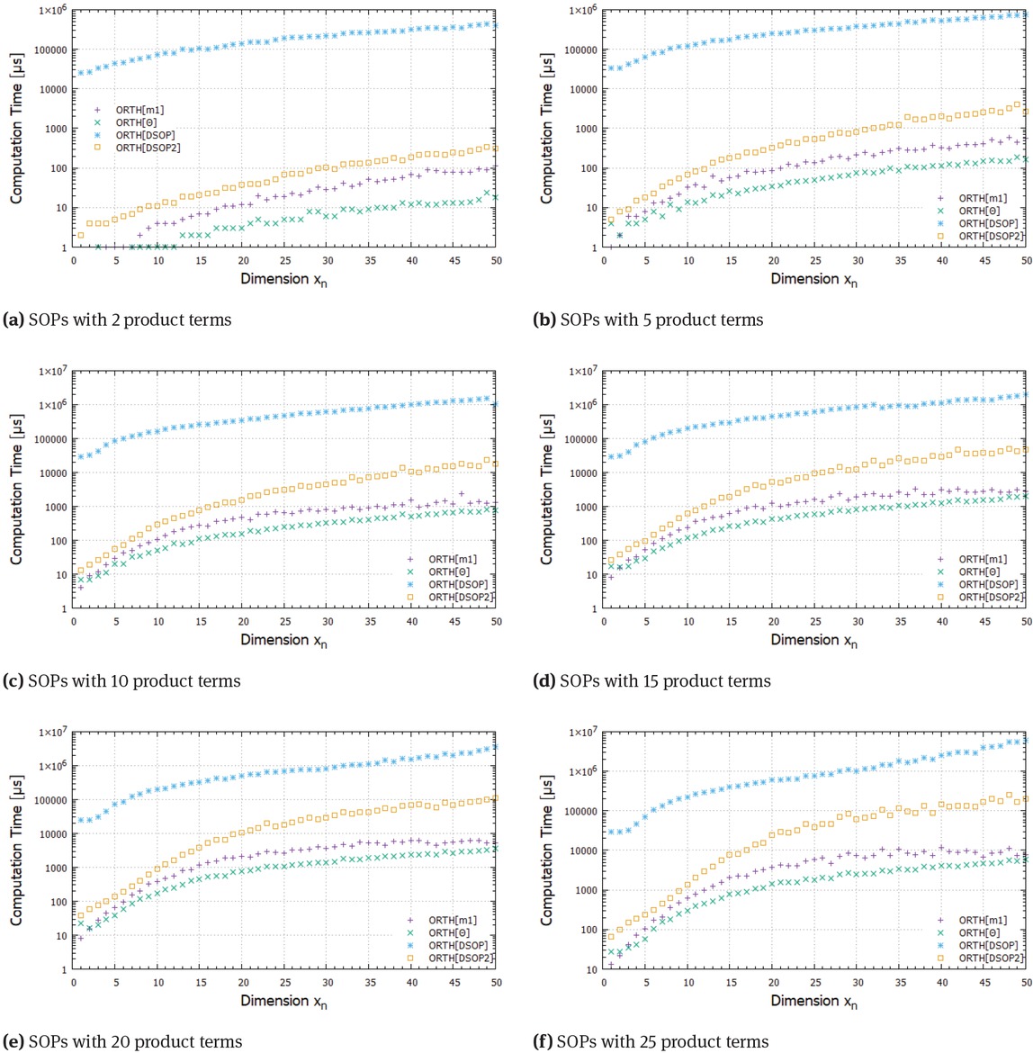
Comparison in computation time
Average of the computation times and relation to ORTH[ⴱ]
| ORTH[ⴱ] | ORTH[DSOP] | ORTH[DSOP2] | ORTH[m1] | ||||
|---|---|---|---|---|---|---|---|
| xn | in μS | in μS | in μS | in μS | |||
| 2 | 7,02 | 196545,63 | 100,48 | 33,09 | 27996,18 | 14,31 | 4,71 |
| 5 | 65,79 | 338287,65 | 988,83 | 191,86 | 5142,02 | 15,03 | 2,92 |
| 10 | 297,52 | 580726,60 | 5586,03 | 667,70 | 1951,86 | 18,78 | 2,24 |
| 15 | 720,68 | 714265,14 | 15323,50 | 1520,70 | 991,10 | 21,26 | 2,11 |
| 20 | 1298,12 | 948014,46 | 31221,00 | 3023,73 | 730,30 | 24,05 | 2,33 |
| 25 | 2211,61 | 1443192,99 | 65237,83 | 5149,57 | 652,55 | 29,50 | 2,33 |
| ∅ | 766,79 | 703505,41 | 19742,95 | 1764,44 | 917,47 | 25,75 | 2,30 |
4 Summary and Conclusions
This work introduced a generally valid method of »orthogonalizing difference-building ⴱ« which is used to calculate the orthogonal difference of two product terms. Furthermore, rules for this method were explained which must be followed to get correct results. By a novel formula based on the combining technique ⴱ every Sum of Products (SOP) can easily be orthogonalized mathematically. Thus, we get disjoint Sum of Products (dSOP). A minimized dSOP can also be reached by two additional procedures of sorting and absorbing of terms before the process of orthogonalization. By sorting the product terms of a SOP are resorted from smaller number of variables to higher number of variables. This resorting brings an advantage of approximately 17% and 26% depending on N to reach minimized dSOP. The corresponding Algorithm ORTH[ⴱ]was compared to other algorithms ORTH[DSOP], ORTH[DSOP2] and ORTH[m1] in their number of product terms in the calculated dSOP and the computation time. ORTH[DSOP] determines fewer number of product terms in contrast to ORTH[ⴱ]. However, the reduction of the product terms by ORTH[ⴱ] is about 50% in contrast to ORTH[m1]. Furthermore, the novel method ORTH[ⴱ] provides approximately 1000 times faster computation in comparison to ORTH[DSOP] and is approximately 25 times faster in comparison to ORTH[m1]. The number of terms in the orthogonalized result by the method ORTH[ⴱ] can probably reduced by an additional absorption of the disjoint product terms. For that, a post-function for absorption could be developed, which retains the property of orthogonality.
References
[1] D. Bochmann, Binäre Systeme - Ein Boolean Buch Hagen, Germany: LiLoLe-Verlag, 2006.Search in Google Scholar
[2] B. Steinbach and C. Posthoff, “An extended theory of boolean normal forms,” in Proc. 6th Annual Hawaii International Conference on Statistics, Mathematics and Related Fields (Hawaii, USA), pp. 1124–1139, 2007.Search in Google Scholar
[3] Y. Can, Neue Boolesche Operative Orthogonalisierende Methoden und Gleichungen Erlangen, Germany: FAU University Press,1 ed., 2016.Search in Google Scholar
[4] Y. Crama and P. Hammer, Boolean Functions - Theory, Algorithms, and Applications. Cambridge, UK: Cambridge University Press, 2011.10.1017/CBO9780511852008Search in Google Scholar
[5] A. Bernasconi, V. Ciriani, F. Luccio, and L. Pagli, “New Heuristic for DSOP Minimization,” in Proc. 8th International Workshop on Boolean Problems (IWSBP) (Freiberg (Sachsen), Germany), 2008.Search in Google Scholar
[6] H. J. Zander, Logischer Entwurf binärer Systeme Berlin, DDR: Verlag Technik, 1989.Search in Google Scholar
[7] B. Steinbach, “The Boolean Differential Calculus – Introduction and Examples,” in Proc. Reed-Muller Workshop 2009 (Naha, Okinawa, Japan), pp. 107–117, 2009.Search in Google Scholar
[8] Y. Can, H. Kassim, and G. Fischer, “New Boolean Equation for Orthogonalizing of Disjunctive Normal Form based on the Method of Orthogonalizing Difference-Building,” Journal of Electronic Testing. Theory and Applicaton (JETTA) vol. 32, no. 2, pp. 197– 208, 2016.10.1007/s10836-016-5572-6Search in Google Scholar
[9] Y. Can, H. Kassim, and G. Fischer, “Orthogonalization of DNF in TVL-Arithmetic,” in Proc. 12th International Workshop on Boolean Problems (IWSBP) (Freiberg (Sachsen), Germany), 2016.Search in Google Scholar
[10] C. Dorotska and B. Steinbach, “Orthogonal Block Change & Block Building Using Ordered Lists of Ternary Vectors,” in Proc. 5th International Workshop on Boolean Problems (IWSBP) (Freiberg (Sachsen), Germany), pp. 91–102, 2002.Search in Google Scholar
[11] C. Posthoff and B. Steinbach, Logikentwurf mit XBOOLE. Algorithmen und Programme. Berlin, Germany: Verlag Technik GmbH, 1991.Search in Google Scholar
[12] C. Posthoff and B. Steinbach, Binäre Gleichungen - Algorithmen und Programme. Karl-Marx-Stadt (Chemnitz), DDR: Technische Universität Karl-Marx-Stadt, 1979.Search in Google Scholar
© 2020 Y. Can et al., published by De Gruyter
This work is licensed under the Creative Commons Attribution 4.0 International License.
Articles in the same Issue
- Regular Articles
- Fabrication of aluminium covetic casts under different voltages and amperages of direct current
- Inhibition effect of the synergistic properties of 4-methyl-norvalin and 2-methoxy-4-formylphenol on the electrochemical deterioration of P4 low carbon mold steel
- Logistic regression in modeling and assessment of transport services
- Design and development of ultra-light front and rear axle of experimental vehicle
- Enhancement of cured cement using environmental waste: particleboards incorporating nano slag
- Evaluating ERP System Merging Success In Chemical Companies: System Quality, Information Quality, And Service Quality
- Accuracy of boundary layer treatments at different Reynolds scales
- Evaluation of stabiliser material using a waste additive mixture
- Optimisation of stress distribution in a highly loaded radial-axial gas microturbine using FEM
- Analysis of modern approaches for the prediction of electric energy consumption
- Surface Hardening of Aluminium Alloy with Addition of Zinc Particles by Friction Stir Processing
- Development and refinement of the Variational Method based on Polynomial Solutions of Schrödinger Equation
- Comparison of two methods for determining Q95 reference flow in the mouth of the surface catchment basin of the Meia Ponte river, state of Goiás, Brazil
- Applying Intelligent Portfolio Management to the Evaluation of Stalled Construction Projects
- Disjoint Sum of Products by Orthogonalizing Difference-Building ⴱ
- The Development of Information System with Strategic Planning for Integrated System in the Indonesian Pharmaceutical Company
- Simulation for Design and Material Selection of a Deep Placement Fertilizer Applicator for Soybean Cultivation
- Modeling transportation routes of the pick-up system using location problem: a case study
- Pinless friction stir spot welding of aluminium alloy with copper interlayer
- Roof Geometry in Building Design
- Review Articles
- Silicon-Germanium Dioxide and Aluminum Indium Gallium Arsenide-Based Acoustic Optic Modulators
- RZ Line Coding Scheme With Direct Laser Modulation for Upgrading Optical Transmission Systems
- LOGI Conference 2019
- Autonomous vans - the planning process of transport tasks
- Drivers ’reaction time research in the conditions in the real traffic
- Design and evaluation of a new intersection model to minimize congestions using VISSIM software
- Mathematical approaches for improving the efficiency of railway transport
- An experimental analysis of the driver’s attention during train driving
- Risks associated with Logistics 4.0 and their minimization using Blockchain
- Service quality of the urban public transport companies and sustainable city logistics
- Charging electric cars as a way to increase the use of energy produced from RES
- The impact of the truck loads on the braking efficiency assessment
- Application of virtual and augmented reality in automotive
- Dispatching policy evaluation for transport of ready mixed concrete
- Use of mathematical models and computer software for analysis of traffic noise
- New developments on EDR (Event Data Recorder) for automated vehicles
- General Application of Multiple Criteria Decision Making Methods for Finding the Optimal Solution in City Logistics
- The influence of the cargo weight and its position on the braking characteristics of light commercial vehicles
- Modeling the Delivery Routes Carried out by Automated Guided Vehicles when Using the Specific Mathematical Optimization Method
- Modelling of the system “driver - automation - autonomous vehicle - road”
- Limitations of the effectiveness of Weigh in Motion systems
- Long-term urban traffic monitoring based on wireless multi-sensor network
- The issue of addressing the lack of parking spaces for road freight transport in cities - a case study
- Simulation of the Use of the Material Handling Equipment in the Operation Process
- The use of simulation modelling for determining the capacity of railway lines in the Czech conditions
- Proposals for Using the NFC Technology in Regional Passenger Transport in the Slovak Republic
- Optimisation of Transport Capacity of a Railway Siding Through Construction-Reconstruction Measures
- Proposal of Methodology to Calculate Necessary Number of Autonomous Trucks for Trolleys and Efficiency Evaluation
- Special Issue: Automation in Finland
- 5G Based Machine Remote Operation Development Utilizing Digital Twin
- On-line moisture content estimation of saw dust via machine vision
- Data analysis of a paste thickener
- Programming and control for skill-based robots
- Using Digital Twin Technology in Engineering Education – Course Concept to Explore Benefits and Barriers
- Intelligent methods for root cause analysis behind the center line deviation of the steel strip
- Engaging Building Automation Data Visualisation Using Building Information Modelling and Progressive Web Application
- Real-time measurement system for determining metal concentrations in water-intensive processes
- A tool for finding inclusion clusters in steel SEM specimens
- An overview of current safety requirements for autonomous machines – review of standards
- Expertise and Uncertainty Processing with Nonlinear Scaling and Fuzzy Systems for Automation
- Towards online adaptation of digital twins
- Special Issue: ICE-SEAM 2019
- Fatigue Strength Analysis of S34MnV Steel by Accelerated Staircase Test
- The Effect of Discharge Current and Pulse-On Time on Biocompatible Zr-based BMG Sinking-EDM
- Dynamic characteristic of partially debonded sandwich of ferry ro-ro’s car deck: a numerical modeling
- Vibration-based damage identification for ship sandwich plate using finite element method
- Investigation of post-weld heat treatment (T6) and welding orientation on the strength of TIG-welded AL6061
- The effect of nozzle hole diameter of 3D printing on porosity and tensile strength parts using polylactic acid material
- Investigation of Meshing Strategy on Mechanical Behaviour of Hip Stem Implant Design Using FEA
- The effect of multi-stage modification on the performance of Savonius water turbines under the horizontal axis condition
- Special Issue: Recent Advances in Civil Engineering
- The effects of various parameters on the strengths of adhesives layer in a lightweight floor system
- Analysis of reliability of compressed masonry structures
- Estimation of Sport Facilities by Means of Technical-Economic Indicator
- Integral bridge and culvert design, Designer’s experience
- A FEM analysis of the settlement of a tall building situated on loess subsoil
- Behaviour of steel sheeting connections with self-drilling screws under variable loading
- Resistance of plug & play N type RHS truss connections
- Comparison of strength and stiffness parameters of purlins with different cross-sections of profiles
- Bearing capacity of floating geosynthetic encased columns (GEC) determined on the basis of CPTU penetration tests
- The effect of the stress distribution of anchorage and stress in the textured layer on the durability of new anchorages
- Analysis of tender procedure phases parameters for railroad construction works
- Special Issue: Terotechnology 2019
- The Use of Statistical Functions for the Selection of Laser Texturing Parameters
- Properties of Laser Additive Deposited Metallic Powder of Inconel 625
- Numerical Simulation of Laser Welding Dissimilar Low Carbon and Austenitic Steel Joint
- Assessment of Mechanical and Tribological Properties of Diamond-Like Carbon Coatings on the Ti13Nb13Zr Alloy
- Characteristics of selected measures of stress triaxiality near the crack tip for 145Cr6 steel - 3D issues for stationary cracks
- Assessment of technical risk in maintenance and improvement of a manufacturing process
- Experimental studies on the possibility of using a pulsed laser for spot welding of thin metallic foils
- Angular position control system of pneumatic artificial muscles
- The properties of lubricated friction pairs with diamond-like carbon coatings
- Effect of laser beam trajectory on pocket geometry in laser micromachining
- Special Issue: Annual Engineering and Vocational Education Conference
- The Employability Skills Needed To Face the Demands of Work in the Future: Systematic Literature Reviews
- Enhancing Higher-Order Thinking Skills in Vocational Education through Scaffolding-Problem Based Learning
- Technology-Integrated Project-Based Learning for Pre-Service Teacher Education: A Systematic Literature Review
- A Study on Water Absorption and Mechanical Properties in Epoxy-Bamboo Laminate Composite with Varying Immersion Temperatures
- Enhancing Students’ Ability in Learning Process of Programming Language using Adaptive Learning Systems: A Literature Review
- Topical Issue on Mathematical Modelling in Applied Sciences, III
- An innovative learning approach for solar power forecasting using genetic algorithm and artificial neural network
- Hands-on Learning In STEM: Revisiting Educational Robotics as a Learning Style Precursor