Accuracy of boundary layer treatments at different Reynolds scales

Nicolás D. Badano; Angel N. Menéndez

doi:10.1515/eng-2020-0033

Artikel Open Access

Accuracy of boundary layer treatments at different Reynolds scales

Nicolás D. Badano und Angel N. Menéndez

Veröffentlicht/Copyright: 8. April 2020

Veröffentlicht von

Veröffentlichen auch Sie bei De Gruyter Brill

Manuskript einreichen Informationen für Autor*innen

Aus der Zeitschrift Open Engineering Band 10 Heft 1

Abstract

Resistive forces associated to boundary layers (‘friction’) are usually out of scale in physical models of hydraulic structures, especially in the case of hydraulically smooth walls, generating distortions in the model results known as scale effects, that can be problematic in some relevant engineering problems. These scale effects can be quantified and corrected using suitable numerical models. In this paper the accuracy of using numerical simulation through the Reynolds Averaged Navier-Stokes (RANS) approximation in order to represent the head losses introduced by friction in hydraulically smooth walls is evaluated for a wide range of Reynolds scales. This is performed by comparing the numerical results for fully developed flow on circular pipes and between parallel plates against experimental results, using the most popular wall treatments. The associated numerical errors, mesh requirements and ranges of application are established for each treatment. It is shown that, when properly applied, RANS models are able to simulate the head losses produced by smooth wall friction accurately enough as to quantify the scale effects present in physical models. A methodology for upscaling physical model results to prototype scale, free of scale effects, is proposed.

Keywords: cfd; rans models; wall treatments; scale effects; physical models

1 Introduction

The design, optimization and verification of hydraulic structures have been traditionally founded on laboratory-scale physical model studies. Despite the advances in numerical modelling during the last few decades, in particular in CFD simulations, physical models are still one of the main tools supporting the engineering of complex structures [1].

A physical model would be completely similar to its real-world prototype counterpart if the following three similarity criteria were met: geometric, kinematic and dynamic similarity [2]. Geometric similarity requires that the shape of the problem is maintained, with a uniform length scale affecting all dimensions. For dynamic similarity, each force acting at any point over the continuum mustscale consistently, with a single uniform and constant ratio, independently of the type of force. Kinematic similarity means that the trajectories of the flow must be preserved, with a uniform scale of time affecting all motions; this condition is naturally achieved when the previous two similarity restrictions are fulfilled [3]. Unfortunately, although geometric similarity can be easily attained, dynamic similarity is virtually impossible to achieve in the real world, as its enforcement would require performing the experiment in a miniature universe [4]. In particular, both the physical model and the prototype share the same (Earth) acceleration of gravity. As a consequence, in problems for which the free surface plays a significant role, then requiring the correct representation of the relationship between inertia and gravity forces (Froude scaling), all the remaining forces acting on the flow are by default out of scale, including viscosity, globally characterized by the Reynolds number. If these out of scale forces have any significance on the flow, then the physical model results no longer correctly represent the flow in the prototype, i.e., scale effects exist [3].

The physical model strategy to overcome this restriction stands on the fact that in most hydraulic engineering flows the Reynolds number is very high in the prototype, so viscosity effects are very small. Hence, to achieve a similar condition on the physical model, a low enough (approach-ing 1) length scale e_L (defined as the ratio between length in the prototype and in the model) must be chosen. However, there are two difficulties with this approach. In the first place, physical model costs are approximately proportional to e_L⁻³ [5], so economic limitations may lead to the selection of a smaller length scale than required to attain enough precision. The second problem arises from the assumption that a high Reynolds number (a global parameter) ensures that viscosity effects are negligible throughout the flow. However, this is not the case, for instance, near solid walls, where viscosity forces are dominant. In fact, when the wall roughness height is low enough, i.e., it is completely immersed in the viscous sublayer, the characteristics of this viscosity-dominated zone strongly affect the turbulent boundary layer, and hence eventually the main flow. In other words, hydraulically smooth walls are by default out of scale on physical models with Froude scaling.

Scale effects have been broadly studied experimenting on physical models [6, 7, 8] usually by building a series of similar models at different scales. In this type of experiments, the largest scale model takes the place of the prototype, and scale effects are determined by comparing against it the performance of the remaining models. However, it is not possible to know if the largest model is itself affected by significant scale effects [4]. Studies comparing the behaviour between prototype scale structures and their physical model predictions have also been performed [9].

Many researchers have focused on determining the minimum scale needed to obtain a reasonably scale effects free representation for typical engineering flows, including, among others, flow on broad crest weirs [10], depths and aeration in hydraulic jumps [11, 12], surface vortices on intakes [13], and trajectories of ski jumps [14]. However, even when using those scales, significant secondary phenomena might be triggered by out of scale forces [15].

The present work is a contribution to evaluate the current capabilities of Computational Fluid Dynamics (CFD) models to quantify scale effects in physical models, and to upscale the results to the prototype scale free from those effects. It stands on the fact that CFD models can represent, at least in principle, the combined effects of all forces acting both at the prototype and at the physical model scales. Hence, by simulating both the prototype and physical model flows, they should be able to elucidate the supposedly marginal effects of out of scale forces in the physical model. Various papers have reported using numerical models for this purpose [16, 17, 18, 19, 20, 21, 22], but little work has been done to evaluate the accuracy of this procedure. Even with limitations, CFD models should provide a more accurate extrapolation of results from the physical model to the prototype, as reported for the design of the Third Set of Locks of Panama Canal [19].

Now, CFD models are still subject to significant uncertainties, especially those associated to the modelling of turbulence. Various approaches exist to account for the effect of turbulence [23], including Direct Numerical Simulation (DNS), Large Scale Eddy Simulation (LES), and Reynolds-Averaged Navier-Stokes modelling (RANS). In recent years, a promising new line of research based on fractal calculus has been made available [24, 25] that may provide a sound conceptual base for studying the properties of turbulence and their interaction with walls of different roughness; it might also be potentially useful to analyse hydraulic scale effects as a whole.

The RANS approach has been used to study a myriad of hydraulic and industrial problems [25, 27, 28, 29, 30, 31, 32, 33, 34]. It is still the most commonly used modelling approach for engineering studies, as it combines reasonable computational costs with acceptable accuracy. In RANS models only the ensemble-averaged flow variables are solved explicitly, while turbulence effects are parameterized in terms of those flow variables. Variations in the parameterization of turbulence effects leads to different RANS models, each one claiming some advantages for particular problems. The models have been tested for a variety of flow conditions and problem scales over the years. However, there are little systematic records of RANS models validation for the same problem at different scales, so their accuracy on predicting scale effects is relatively uncertain.

In this paper, the accuracy of the most common RANS models when simulating head losses due to skin friction in hydraulically smooth walls, is evaluated for a wide range of scales, using the fully developed flow in circular pipes and between parallel plates as benchmark problems. The most widely used turbulence models and two alternative treatments to implement the boundary conditions at smooth walls, are considered, establishing their ranges of applicability and margins of error. Their accuracy is quantified by comparing the predicted head losses against experimental results. Some of the models employed in this paper have been validated for boundary layer problems by comparing velocity profiles or friction factors for some Reynolds numbers [35, 36, 37]. In this paper, the validation is systematically extended for the friction factor over a wide range of conditions. Only skin friction is considered in this paper; scale effects on drag due to flow separation are analysed in a forthcoming paper. Additionally, the methodology to predict prototype scale performance free of scale effects, through the use of numerical modelling, is described.

The plan of the paper is as follows. In the first place the benchmark problems are presented – this includes the formulas and experimental results –, and the errors that arise when simulating them on physical models with Froude scaling are quantified. In the second place, a brief yet comprehensive description of RANS models is presented, including the different wall treatments. In the third place, the errors in the numerical model are evaluated – this includes the formulation of best practices in order to minimize them – and compared to those incurred in physical models at different scales. Finally, the procedure to upscale the results to the prototype scale, is explained.

2 Benchmark problems

2.1 Description

Two problems are studied in this paper: flow along a pipe with a circular cross section, and flow between parallel flat plates (duct), both under fully developed flow conditions and for hydraulically smooth walls. The geometry for the first case is determined by the conduit diameter D, and for the second case by the distance between the plates H. The effect of the fluid viscosity is characterized by the Reynold number, which is defined as follows:

(1)RC=DU¯νRP=2HU¯ν

where the subindex c and p indicate circular and flat plate geometries, respectively, U the mean velocity, and ν the kinematic viscosity of the fluid. This somewhat inconsistent definitions of the Reynolds number have been adopted due to their extensive usage in the literature.

The definitions of the friction factor for pipes f_c, known as Darcy’s, and ducts f_p, known as Fanning’s, are as follows:

(2)fc≡8τwρU¯2fp≡2τwρU¯2

The friction factors can also be expressed as a function of the pressure difference ᐃp between both extremes of a pipe or duct of length L (taking into account the balance between friction and pressure forces):

(3)fc=Δp2DρLU¯2fp=ΔpHρLU¯2

Experimental values for the friction factor published in the literature were employed as a basis for comparison to assess the accuracy of the model results.

For the pipe problem Blasius equation and Colebrook & White curve fit [38, 39] where used:

(4)fc=64/cifRc≤25001fc=2logRcfc−0.8if20000<Rc

The experimental data from the Princeton Superpipe experiments [40], and the transitional data by Patel & Head [41] were also employed as a reference for this case.

In the case of the duct problem, a data fit plotted by Rothfus et al. [42] was taken for comparison. It is pertinent to mention that this plot was built by assuming that the nondimensional velocity profile is the same for the pipe and duct cases. Based on the dispersion of the data, an error of around 7% was estimated.

2.2 Errors in Froude scaled physical models

To put into context the precision of the numerical models, the magnitude of expected scale effects in a physical model with Froude scaling is first evaluated. Specifically, the pipe problem is analysed, which could be interpreted as representing a stretch of a hydraulically smooth pipe within a hydraulic system with a free surface, such as the one of a shiplock.

For Froude scaling, the Reynolds number of the physical model relates to the one in the prototype as:

(5)Rmodel=RprototypeeL−1.5

Assuming that both the prototype and scale model walls are hydraulically smooth, and that the pipes have a circular cross section, the friction factor can be computed with the Colebrook & White equation. These friction factors are presented in Figure 1 as a function of the prototype Reynolds number and the length scale. It is observed that a substantial amplification of the friction factor occurs in the physical model as the scale decreases. The relation between the friction factor of the model and prototype is plotted in Figure 2. Note that in the turbulent flow regime the friction factor for the physical model can be from about 50% to 350% larger than the one for the prototype.

Figure 1

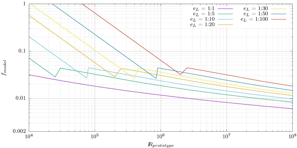
Friction factor for hydraulically smooth circular pipes. Prototype versus physical models at different scales.

Figure 2

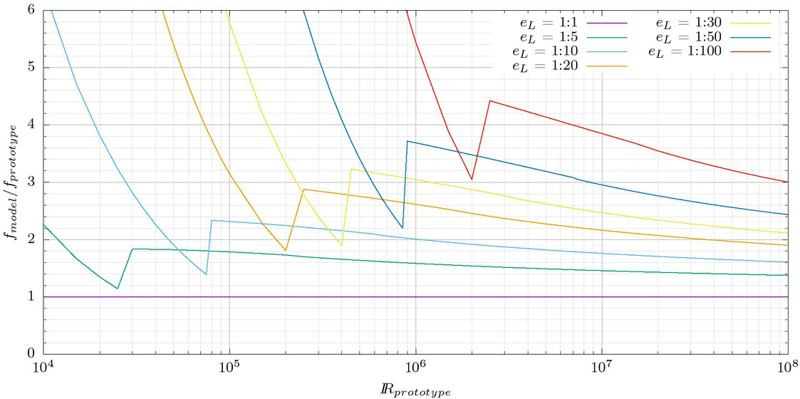
Relation between physical model and prototype friction factors for hydraulically smooth circular pipes.

The magnitude of this error highlights the need for methodologies that allow its computation and correction. For this simple problem the experimental fit of Colebrook & White could be employed, but for more complex cases numerical models are the only alternative. This is the motivation to determine how accurately typical RANS models can solve head losses due to friction in smooth walls.

3 Description of the RANS model

3.1 Basic conservation equations

Assuming incompressible monophasic flow, the mass conservation equation is:

(6)∇∙U¯=0

where U is the Reynolds-averaged velocity. Adopting the Boussinesq approximation to represent Reynolds stresses isotropically using an eddy viscosity ν_t, the momentum conservation equation can be written as [43]:

(7)∂U¯dt+∇⋅U¯⊗U¯−∇⋅ν+νt∇U¯+∇U¯T=−∇p~¯

where ν is the kinematic viscosity of the fluid, and p~¯the Reynolds-averaged value of the modified kinematic pressure, which incorporates the contribution of k, the turbulent kinetic energy (TKE):

(8)p~¯=p¯ρ+23k

with p being the Reynolds-averaged value of pressure, and ρ the fluid density (assumed as a constant due to incompressibility).

3.2 Turbulence models

Several turbulence models belonging to the k-ε family were evaluated in this paper. k-ε models represent turbulence by keeping track of the evolution of the turbulent kinetic energy and its viscous dissipation rate, ε, through their conservation equations.

The standard k-ε model [36] reads:

(9)∂k∂t+∇⋅U¯k−∇⋅ν+νtσk∇k=Pk−ε∂ε∂t+∇⋅U¯ε−∇⋅ν+νtσε∇ε=C1εkPk−C2εkε

where C₁, C₂, σ_k, σ_ε are constants, and P_k is the production rate of TKE, which is expressed as:

(10)Pk=2νt12∇U¯+∇U¯T2

The two turbulence variables k and ε determine a length and a time scales for the dominant eddies, from which the expression for the eddy viscosity arises:

(11)νt=Cμk2ε

where C_μ is a constant. The values of the constants for the standard k-ε model are:

(12)Cμ=0.09C1=1.44C2=1.92σk=1.00σε=1.30

This k-ε model is the most widely validated and used RANS turbulence model, due to its efficiency and relative simplicity [44]. Its performance is considered as particularly satisfactory for confined flows in which Reynolds stresses are dominant, a frequent condition in engineering problems. Its performance is less satisfactory for non-confined flows, boundary layers with large curvature, and rotating flows [45].

The RNG k-ε model [46] was also tested. This is a variant of the standard model derived using Renormalization Group Theory, which states that all scales of motion contribute to the momentum diffusion instead of a single representative scale. The resulting equations are completely similar to those of the standard model, but with different values of the constants, and C₂ expressed in terms of the deformation tensor.

The realizable k-ε model [47] is a variant which introduces a variable C_μ coefficient, depending on both the deformation and rotation tensors.

Now, in the boundary layer the velocity decreases to match that of the wall. Hence inertia gradually loses significance when approaching the wall, and viscous forces eventually become dominant. This means that turbulence models able to deal with low Reynolds number conditions are required to solve the boundary layer region explicitly. They are collectively known as Low Reynolds Number models, and are becoming increasingly popular, especially for problems in which the boundary layer is neither in equilibrium nor fully developed, as in fast hydraulic transients [48, 49, 50, 51] and separated flows. The most popular k-ε Low Reynolds Number models were compared by Patel & Rodi [37], who concluded that the one with the best performance was Launder-Sharma’s [35, 52], followed by that of Chien [53] and Lam & Bremhorst [54]. The Launder-Sharma k-ε model equations are the following:

(13)∂k∂t+∇⋅(U¯k)−∇⋅[(v+vtσk)∇k]=Pk−ε−2v|∇k12|2∂ε∂t+∇⋅(U¯ε)−∇⋅[(v+vtσε)∇ε]=C1εkPk−C2f2εkεvt=Cμfμk2ε

These equations include the following weight functions:

(14)f2=1−0.3e−ℝt2fμ=e−3.4/(1+ℝt/50)

in which ℝ_t is the local Reynolds number of the turbulence, defined as:

(15)Rt=k2εν

3.3 Numerical code

The conservation equations were solved using OpenFOAM^® [55, 56], a set of applications and libraries to deal with continuum mechanics problems. The capabilities of OpenFOAM are similar to those of Flow-3D [18, 57]. The differences lies in accessibility and numerics; while the latter one is a commercial code that uses the Finite Difference Method (FDM) over one or more structured meshes of hexahedra, OpenFOAM is an open-source free software based on the Finite Volume Method (FVM) with a collocated treatment for variables over non-structured meshes of polyhedral elements. In OpenFOAM the temporal discretization is implicit, with a pressure-velocity coupling analogous to that of Rhie & Chow [58].

As the numerical simulations presented in this paper are time independent, the SIMPLE (Semi-Implicit Method for Pressure Linked Equations) [59] iterative procedure was used.

3.4 Wall treatments

Turbulent Boundary Layer theory identifies, adjacent to the wall, the Inner Boundary Layer [60], where the flow (contrary to the Outer Layer) is practically independent of the characteristics of the global flow, the shear stress is rather constant, and the Law of the Wall holds:

(16)u+=U¯u∗=fyu∗ν=f(y+),

where y is the distance to the wall, τ_w the wall shear stress (representative of the shear stress throughout the inner boundary layer), u⋆=τw/ρthe shear velocity, u⁺ the dimensionless velocity, and y⁺ the dimensionless wall distance. Three sub-regions can be distinguished, starting from the wall [45]: (i) the viscous sublayer, extending up to approximately y⁺ ≈ 5 [60], where viscous forces are dominant, and the velocity profile is linear; (ii) the transition sublayer, which extends within the interval 5 < y⁺ < 30, where both viscous and Reynolds stresses are significant; and (iii) the inertial sublayer, extending outwards y⁺ > 30 and up to about y⁺ ≈ 500 or less, where viscous stresses are already negligible, and the velocity profile is logarithmic, as observed experimentally and confirmed theoretically through dimensional analysis [60].

Based on this knowledge, different treatments have been developed to account for the boundary layer on CFD models. In this paper, the two most popular treatments are analyzed and compared, namely, Low Reynolds Number (LRN) and Logarithmic Wall Function (LWF).

Regardless of the type of treatment, the goal is to enforce the relation between the velocity parallel to the wall on the first computational node, U, and the wall shear stress. This can be accomplished by either introducing a momentum sink term on that node or locally manipulating the eddy viscosity, . OpenFOAM^® uses the latter approach. RANS equations near the wall assume that:

(17)τwρ=ν+νtwU¯−Uw¯y

in which Uw¯is the wall velocity. Considering static walls Uw¯=0),the following relationship is derived:

(18)νtw=ν⋅y+u+−1

which provides the value of the eddy viscosity to be assigned a the cells adjacent to the wall (i.e., its boundary condition) once a relationship between u⁺ and y⁺ is known.

3.4.1 LRN treatment

Under the LRN treatment the flow is explicitly solved throughout the entire boundary layer. Due to the relatively high velocity gradients within the boundary layer, a dense discretization is needed to attain accuracy. The first calculation node, at the center of the cells adjacent to the wall, has to lie inside the viscous sublayer (y⁺ < 5). As viscous effects are significant both in the transitional and viscous sublayers, a Low Reynolds Number turbulence model is required.

Now, for the viscous layer the velocity profile is given by [60]:

(19)u+=y+

Replacing (14) in (18), the boundary condition for the eddy viscosity arises:

(20)νtw=0

Experiments show that the TKE has a peak value in the transition sublayer, associated to the high velocity gradients. However, turbulent eddies rapidly decay inside the viscous sublayer, as shown by Klebanoff [61], so the appropriate boundary condition for k is also a zero value. Due to implementation details in OpenFOAM, null TKE values are not allowed, so a very small number must be assigned (for example, 10⁻¹²).

As for the dissipation rate, ε, slightly different boundary conditions are used depending on the Low Reynolds Number model, consisting either of a zero normal gradient or a zero value [37]. In the case of the Launder-Sharma model, a zero value is recommended. As for the TKE, Open-FOAMdoes not allow a zero value for ε, so a very small one must be used instead.

This Low Reynolds Number treatment assumes from the start that the wall is hydraulically smooth.

3.4.2 LWF treatment

The LWF treatment consists of extending the flow simulation down to a certain point contained within the inertial sublayer, where a wall function is imposed.

On the inertial sublayer, the velocity profile can be expressed as [60]:

(21)u+=1κln⁡(Ey+)

in which E is a constant (= 9.8) for large enough Reynolds numbers and smooth wall. The first computational node must lie within the inertial sublayer, i.e., it has to verify the condition.

Compared to the LRN treatment, using wall functions greatly reduces the computational cost due to the very significant reduction in the number of computational nodes. This explains its popularity.

Experiments indicate that in the inertial sublayer TKE production and dissipation rate are in equilibrium [45]. Therefore, from equations (9) and (10), and taking into account the logarithmic profile for U, the following equations can be derived:

(22)k=u∗2Cμε=u∗3κy

Equation (17) is used to impose the boundary conditions for ε. In the case of k, instead of (17) a zero gradient condition, ∂k/∂y = 0 (based on the equality of production and dissipation) is usually adopted due to numerical stability reasons.

Now, equation (21) must be solved iteratively, as τ_w is not known a priori. An additional complication is that τ_w may become locally null at points of flow detachment, so this special case has to be dealt with specifically in the code in order to prevent from spurious results. In order to avoid these difficulties, Launder & Spalding [36] proposed an alternative computational procedure, consisting in deriving the shear velocity from the TKE using equation (17):

(23)u∗=Cμ0.25k0.5

4 Evaluation of the numerical model errors

4.1 Implementation of the numerical tests

To test the accuracy of the different wall treatments and turbulence models, RANS models were implemented for each condition on the two flow cases: flow along a pipe with a circular cross section, and flow between parallel flat plates (duct). Each model was run to convergence for different Reynolds numbers, and the resulting friction factors were computed and compared to experimental values.

Both the diameter of the conduit D and the distance between the parallel plates H were fixed at 0.10 m. A mean velocity of 1.00 m/s was imposed at the upstream boundaries. Periodic boundary conditions were applied for the velocity distribution and the turbulent properties, in order to achieve fully developed flow conditions independently of the model length. The fluid viscosity was varied according to equation (1) in order to get different values for the Reynolds number the same model geometry and mean velocity.

Due to the radial and lateral symmetries of the pipe and duct problems, respectively, both of them are amenable to a two-dimensional approach. Rectangular elements were selected for the computational grids. The size of the first layer of elements adjacent to the wall was adjusted, for every Reynolds number, in order to achieve a correct y⁺ value at the first node (y1+),as required by the adopted wall treatment. As the LRN model is quite sensitive to the spatial discretization close to the wall, the cell size was kept constant up to y⁺ ≈ 20, and then increased as a geometric progression, with an expansion factor R = 1.1. The same geometric progression was used for the case of the wall function treatment, starting from the cell closest to the wall.

The experimental values for the friction factor published in the literature were used to estimate a priori the required distance of the first node to the wall (hence avoiding an iterative procedure).

The testing methodology is summarized in Figure 3. Further details of the model implementation are provided in Table 1.

Figure 3

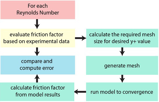
Flowchart of the numerical testing procedure.

Table 1

Model implementation details.

OpenFOAM version	2.3
Solver code	simpleFoam
Gradient Schemes	Gauss linear
Divergence Schemes	bounded Gauss linear
Laplacian Schemes	Gauss linear corrected
Interpolation Schemes	linear
Relaxation factors	0.3 for p, 0.7 for the rest of variables

4.2 Results for the LRN treatment

4.2.1 Model performance

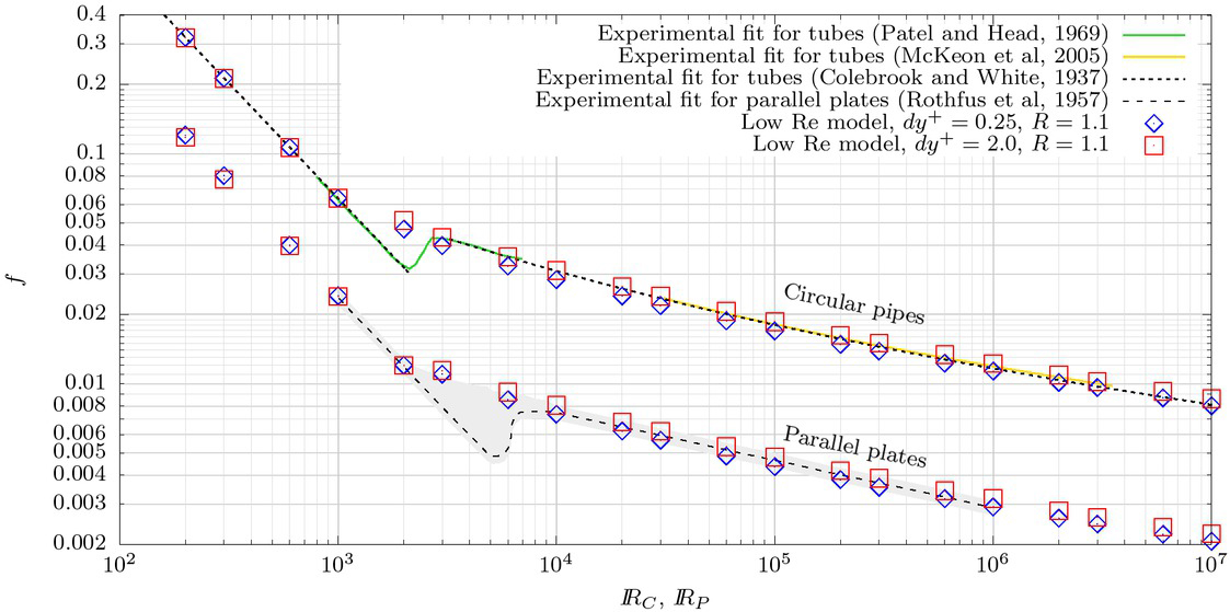
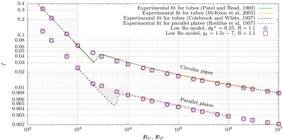
Tests were undertaken using the LRN treatment, described in equations (19) and (20), with the Launder-Sharma k-ε turbulence model for a wide range of Reynolds numbers, from 2 × 10² to 1 × 10⁷.

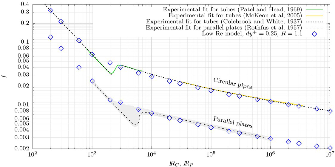
Different mesh configurations were tested until mesh convergence was achieved, with a tolerance of 1% on the friction factor. The thickness of the first set of layers for the converged mesh was ᐃy⁺ = 0.25 for 0 ≤ y⁺ ≤ 20 (hence, y1+=Δy+/2=0.125).The friction factor was computed from the model results using equation (3). Figure 4 shows the comparison with the experimental curves. An overall satisfactory agreement is observed for the two problems, and for both the laminar and the turbulent regimes. However, it is observed that the model is not able to represent the sudden changes of the friction factor within the transition range, but instead it smoothly links the curves associated to laminar and turbulent flow. This is not considered as a practical limitation, as the usual engineering studies do not deal with transitional flows.

Figure 4

Comparison between friction factor from LRN treatment and from experimental results.

Figure 5 shows the relation between the computed and experimental friction factors. For the circular pipes the relative error is below 1% in the laminar regime, increases up to 9% in the turbulent regime, then decreasing with the Reynolds number. For the parallel plates the trend is qualitatively similar, but a higher maximum error is observed for the laminar regime, of about 2%, and lower one for turbulent flow, of about 6%. However, it should be kept in mind that the reference friction factor curve for the parallel plates flow is relatively uncertain (7% error), so the deviation trends quantified for pipes should be considered as more indicative of the actual model performance.

Figure 5

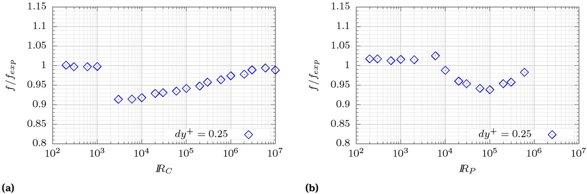
Relative error of friction factor from LRN treatment for circular pipes (left) and parallel plates (right).

When these errors are compared with those associated to a Froude scaled physical model, as presented in Figure 2, it is observed that the latter ones are practically negligible, so the numerical model results can be considered as very accurate from the engineering point of view.

4.2.2 Underprediction for turbulent flow

The results plotted in Figures 4 and 5 show as systematic underprediction of the friction factor over the entire range of turbulent conditions for the circular pipe, and over most of the range for the parallel plates. This is consistent with the results published by Etemad et al. [62], in which various LRN models were shown to underpredict the friction factor for a square duct at ℝ = 5.6 × 10⁵. It is therefore of interest to assess why that bias is observed.

Figure 6 presents the results of the LRN model with the thickness of the first set of layers (up to y⁺ = 20) increased from ᐃy⁺ = 0.25 to ᐃy⁺ = 2. A consistent increase of the friction factor is observed for both the pipe and duct problems. This higher energy loss better matches the experimental curve for the circular pipe, as shown in Figure 7.

Figure 6

Friction factor from LRN treatment with coarser mesh.

Figure 7

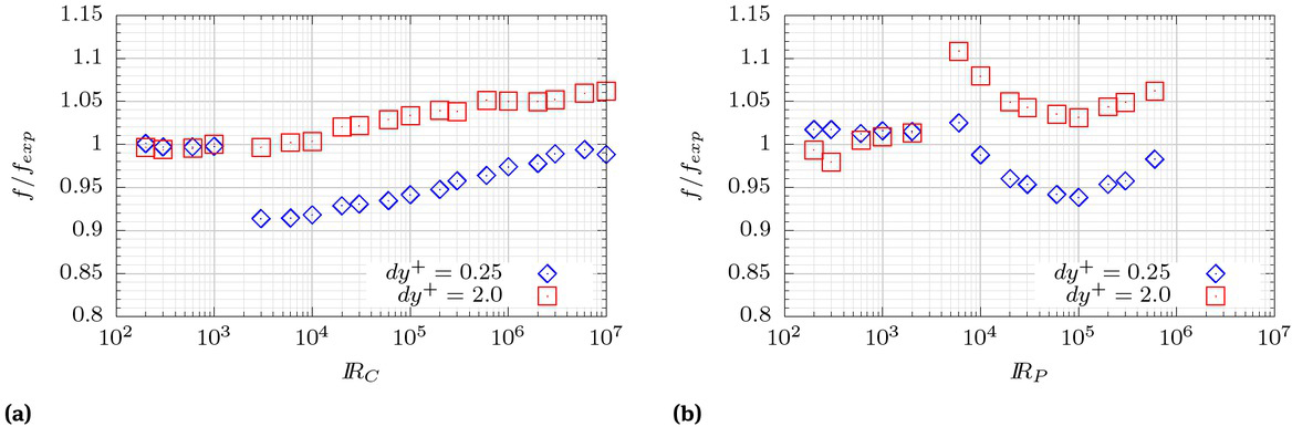
Relative error of friction factor from LRN treatment with coarser mesh for circular pipes (left) and parallel plates (right).

These results suggest that the increase in truncation error arising from using a coarser mesh might help in reducing the under-prediction of the friction factor. To investigate the reason behind this effect, u⁺ and k profiles were plotted on Figure 8 for the two mesh sizes corresponding to the pipe problem, for ℝ_C = 10⁶. It is observed that the coarse mesh provides an insufficient resolution to accurately represent the TKE profile 1 < y⁺ < 10 range, leading to a higher peak value in the transitional sublayer. This extra TKE requires an extra dissipation, and hence leads to a higher friction factor, which better matches the experimental data. This argument would then suggest that the Launder-Sharma LRN model would need some tuning in order to better represent the correct TKE profile on fine meshes.

Figure 8

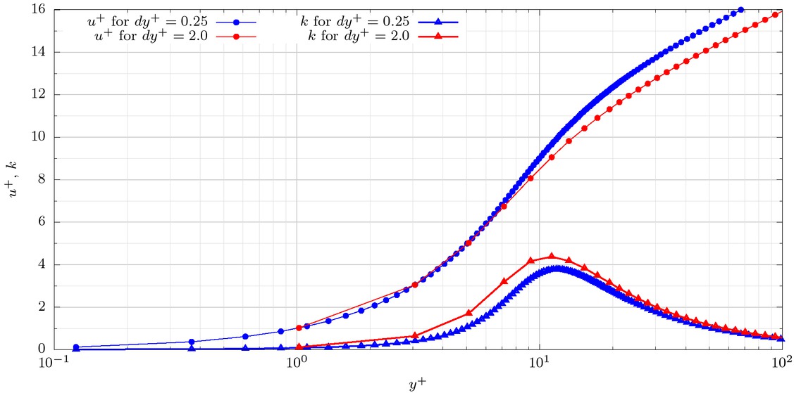
u⁺ and k profiles for the circular pipe from LRN treatment with R_C = 10⁶, using different meshes.

The previous test also indicates that the results for the friction factor from the LRN treatment are very sensitive to mesh discretization in the transitional sub-layer, besides the restriction for the location of the first node (which is perfectly fulfilled by both meshes). It seems that a higher computational efficiency (in terms of computing time) could be achieved if the mesh were densified without the need of moving the first node closer to the wall. In this respect, the collocated arrangement of variables used by OpenFOAM, among many other computer packages based on the FVM, is limited, as the computational nodes can at most be arranged with a fixed spacing equal to 2y₁. Furthermore, if the cell size is geometrically increased, as per usual practice, the resolution on the transitional sublayer is further decreased.

4.2.3 Simulation of different Reynolds numbers with the same mesh

An interesting property of the LRN treatment is that, theoretically, if a sufficiently fine mesh is used it should be possible to solve a wide range of Reynolds conditions with the same mesh. This is important in cases where flow transients occur, and the discharge changes significantly over time.

Figure 9 presents, for the pipe problem, a comparison between the results with the converged mesh for each Reynolds number, and the ones obtained with a single mesh for the whole Reynolds number range, namely, the converged mesh for the highest tested Reynolds number, ℝ = 10⁷. It is observed that the differences are practically negligible. This test then confirms that,when dealing with transient fully developed flow in which the Reynolds number vary in time over a wide range of values, it is possible to work with a single mesh, the one appropriate for the highest Reynolds number, without the need of performing any re-meshing during the calculations.

Figure 9

Friction factor from LRN treatment with single mesh.

4.3 Results for the LWF treatment

4.3.1 Model performance

Tests were carried out for the two geometrical problems using the LWF treatment, described in equations (21) to (23), with three different turbulence models: Standard k-ε, RNG k-ε and realizable k-ε.

The LWF treatment only applies when the flow is in the turbulent regime. Hence, the tests were performed for the range of Reynolds numbers above ℝ = 3000, which is the approximate threshold at least for the circular smooth pipe problem.

For every test the mesh was generated so as the first node close to the wall lied at a nondimensional distance y1+=30.From thereon, the ⁺cell size was increased geometrically with an expansion factor R = 1.1.

Figure 10 shows the comparison of the numerical simulations with the experimental curves, indicating an overall satisfactory agreement. The two methodologies above described to solve for the shear velocity were tested for the standard k-ε model, i.e., iterating over y⁺ and using the method by Launder & Spalding [36], but the results turned out to be identical, which could be expected due to the absence of flow separation in the test problems.

Figure 10

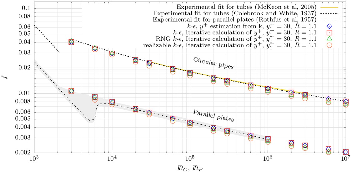
Comparison between friction factor from LWF treatment and from experimental results.

Figure 11 presents the errors relative to the experimental curves. In the case of the circular conduit it is observed that the LWF treatment tends to under-predict the friction factor with the three turbulence models. The standard k-ε model shows the better overall performance, with differences below 4% for ℝ_C > 3×10⁴, and reaching a maximum of 7% around ℝ_C ≈ 10⁴. For the realizable and RNG turbulence models the errors are similar to those of the standard model at low Reynolds numbers, but significantly larger at higher ℝ_C.

Figure 11

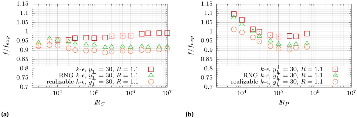
Relative error of friction factor from LWF treatment for circular pipes (left) and parallel plates (right).

For the case of parallel plates, the three models over-predict the friction factor for ℝ_P < 2 × 10⁴, with the realizable turbulence model showing the lowest errors. However, for higher Reynolds numbers the standard model performs much better, with a maximum error of around 3%.

In any case, as for the LRN treatment, these errors are very much smaller than the ones associated to physical models.

4.3.2 Resolution limit

Though the previous results indicate that the LWF treatment is suitable down to relatively low Reynolds numbers, even below 1 × 10⁴ for the circular pipe, there exists a numerical resolution problem for that low range. For example, for the pipe problem the spatial range of the y coordinate is limited by the restriction 30 ≤ y⁺ ≤ r⁺, where r⁺ = D/2u^*ν⁻¹ is the nondimensional radius of the conduit. 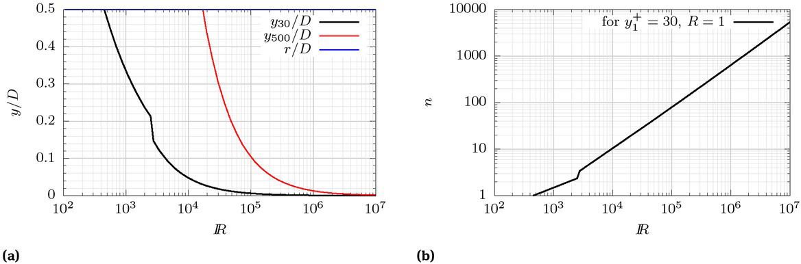Figure 12 shows the lower (y⁺ = 30) and upper (y⁺ = 500) limits of the inertial sublayer in terms of the nondimensional coordinate y¯≡y/D,as a function of ℝ. It is observed that below ℝ = 2 × 10⁴ the outer layer disappears, so the model domain extends completely within the inertial sublayer. As ℝ decreases further, the lower limit of the inertial sublayer grows steadily, reducing the effective model domain.

Figure 12

Upper and lower limits of the inertial sublayer (left) and number of grid points in the cross section (right) as a function of the Reynolds number.

Figure 12 also shows the number of grid points in the cross section when using equal size cells with y1+=30.As observed, the discretization becomes increasingly coarser when ℝ decreases. For example, for ℝ = 2 × 10⁴ the entire cross section of the conduit ends up being discretized in only 20 cells. This quantity might be considered the minimum amount of grid points required to give a reasonable representation of the velocity profile, and hence the lower limit of ℝ for the application of the LWF treatment.

Though for the particular problems solved in this paper (fully developed flow in conduits) the results were found to be reasonably accurate for Reynolds numbers below that limit, this is attributed to the simplicity of the problems.

4.4 Discussion on numerical model errors

As a guidance for ‘best management practices’, Table 2 presents a synthesis of the conditions applicable to RANS models of the k-ε family to simulate wall-bounded flows using LRN or LWF treatments. They include the restrictions and error bounds for the friction factor found in the present paper.

Table 2

Summary of applicability conditions for the wall treatments.

	LRN Treatment	LWF Treatment
Range of application	Any	ℝ ≥ 2 × 10⁴
Mesh requirement	y1+=0.25	30≤y1+≤500
	ᐃy⁺ = 0.5 up to y⁺ = 20	y/R ≤ 32
Limitations	- Requires LRN turb. model	- Near wall mesh very
	- Computationally expensive at high Re	dependent on target Re
Eddy viscosity on the first cell	ν_tw = 0	vtw=v⋅(y+u+−1)
Boundary condition for k	k ≈ 0	∂k∂v=0
Boundary condition for ε	ε ≈ 0	ε = u^*3⁻¹y⁻¹
f relative error	< 9%	< 7%

The LWF treatment has been shown to be quite competitive in relation to the LRN treatment for high Reynolds numbers, as it provides similar errors for the friction factor while keeping a much coarser grid (hence requiring a much lower computing time). However, for ℝ < 2 × 10⁴ the requirement of locating the first node within the inertial sublayer leads to a substantial loss of resolution of the flow profiles.

Using these best practices, it has been shown that numerical models based on the RANS approach with k-ε turbulence models are able to represent the friction factor for a wide range of Reynolds numbers with errors below 10%. This means that for a typical hydraulic project, these models can accurately represent smooth wall frictional head losses for both the prototype scale and any reduced scale adopted for the physical modelling.

5 Methodology to avoid scale effects

It has been shown that the friction factor in a physical model amplifies relative to the one in the prototype, with increments from about 50% to 350%, then introducing significant scale effects.

On the other hand, it has also been demonstrated that RANS models can be used as a relatively accurate tool to quantify the scale effects introduced by smooth wall friction on physical models, by numerically simulating the problem at both scales and comparing the results. Moving further, this allows the use of the numerical model to predict prototype scale performance free of scale effect with relative accuracy, by applying the following methodology, outlined on Figure 13:

Figure 13

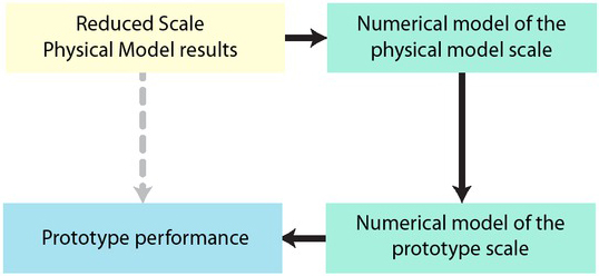
Outline of the methodology to predict prototype performance free of scale effects.

Implement a numerical model representing the reduced scale physical model.
Validate this reduced scale numerical model by comparing its results to those measured in the physical model. Different turbulence models should be tested, in order to find the one that best matches the problem. Eventually, some turbulence model parameters could be adjusted for better calibration.
Implement a numerical model representing the prototype at full scale, using the same turbulence model and parameters as the ones adopted for the physical model.

This procedure was already applied by the authors when dealing with the design of the filling/emptying system for the Third Set of Locks of Panama Canal [15], albeit without evaluating the errors of the numerical model.

6 Conclusions

From analyses undertaken for fully developed flow in smooth pipes and ducts in the range of Reynolds number from 10⁴ to 10⁸, it has been shown that the friction factor in Froude-scaled physical models is significantly over-predicted, leading to the introduction of scale effects. Meanwhile, numerical models based on the RANS approach, using k-ε turbulence models, are able to represent the friction factor for both scales with errors below 10%, which can be considered as practically negligible from the engineering point of view. RANS models can therefore be used as a relatively accurate tool to quantify the scale effects introduced by smooth wall friction on physical models. In order to attain the reported accuracy, the computational mesh must fulfil some conditions (synthetized in Table 2). In the case of the LRN treatment, a minimum cell size and a band of constant cell sizes within the inertial sublayer is recommended. If the LWF treatment is applied, the condition on the location of the first node close to the wall restricts both the model domain and the grid resolution, so a lower limit of 2 × 10⁴ is recommended for the Reynolds number. Digging deeper into the characteristics of the numerical error, it has been shown that the consistent underprediction of the friction factor of Launder-Sharma LRN model for the full turbulent regime, could be explained as a misrepresentation of the peak value of TKE occurring in the inertial sublayer, suggesting that some tuning of this model would be necessary in order to better represent this effect. To attain results free of scale effects, a two-step methodology using numerical models is proposed. In the first place, the physical model scale is numerically simulated in order to validate the numerical treatment. In the second place, the prototype scale is numerically simulated with the validated numerical treatment.

References

[1] Erpicum S, Tullis BP, Lodomez M, Archambeau P, Dewals BJ, Piroton M. Scale effects in physical piano key weirs models. J Hydraul Res. 2016;54(6):692–8.10.1080/00221686.2016.1211562Suche in Google Scholar

[2] Yalin M. Theory of hydraulic models. London: Macmillan; 1971. https://doi.org/10.1007/978-1-349-00245-010.1007/978-1-349-00245-0Suche in Google Scholar

[3] Ackers P. (1987). Scale models. examples of how, why and when - with some ifs and buts On Proc. Of Technical Session B, XXII IAHR Congress. Lausanne, Switzerland.Suche in Google Scholar

[4] Heller V. Scale effects in physical hydraulic engineering models. J Hydraul Res. 2011;49(3):293–306.10.1080/00221686.2011.578914Suche in Google Scholar

[5] Le Méhauté B, Hanes D. (1990). Ocean engineering science, the sea. B., Chapter 29, Similitude 955–980. Wiley, New York. DOI: https://doi.org/10.4319/lo.1990.35.7.165610.4319/lo.1990.35.7.1656Suche in Google Scholar

[6] Kobus H, editor. (1984). Proc. of the Symposium on scale effects in modelling hydraulic structures IAHR, Esslingen, Germany, 1984. ISBN: 9783921694985Suche in Google Scholar

[7] Ettema R, Muste M. Scale Effects in Flume Experiments on Flow around a Spur Dike in Flatbed Channel. J Hydraul Eng. 2004;130(7):635–46.10.1061/(ASCE)0733-9429(2004)130:7(635)Suche in Google Scholar

[8] Tandalam A, Balachandar R, Barron R. Reynolds Number Effects on the Near-Exit Region of Turbulent Jets. J Hydraul Eng. 2010;136(9):633–41.10.1061/(ASCE)HY.1943-7900.0000232Suche in Google Scholar

[9] Ansar M, Chen Z. Generalized Flow Rating Equations at Prototype Gated Spillways. J Hydraul Eng. 2009;135(7):602–8.10.1061/(ASCE)0733-9429(2009)135:7(602)Suche in Google Scholar

[10] Hager W. Breitkroniger ÜberfallBroad crested spillwaysWasser Energie Luft. 1994;86:363–9.Suche in Google Scholar

[11] Hager W, Bremen R. Classical hydraulic jump: sequent depths. J Hydraul Res. 1989;27(5):565–85.10.1080/00221688909499111Suche in Google Scholar

[12] Chanson H. Turbulent air-water flows in hydraulic structures: dynamic similarity and scale effects. Environ Fluid Mech. 2009;9(2):125–42.10.1007/s10652-008-9078-3Suche in Google Scholar

[13] Anwar H, Weller J, Amphlett M. Similarity of free-vortex at horizontal intake. J Hydraul Res. 1978;16(2):95–105.10.1080/00221687809499623Suche in Google Scholar

[14] Heller V, Hager W, Minor H. Ski jump hydraulics. J Hydraul Eng. 2005;131(5):347–55.10.1061/(ASCE)0733-9429(2005)131:5(347)Suche in Google Scholar

[15] Menéndez A, Badano ND. Interaction between Hydraulic and Numerical Models for the Design of Hydraulic Structures. Hydrodynamics; 2011. https://doi.org/10.5772/2868810.5772/28688Suche in Google Scholar

[16] Kim DG, Park JH. Analysis of Flow Structure over Ogee-Spillway in Consideration of Scale and Roughness Effects by Using CFD Model. KSCE J Civ Eng. 2005;9(2):161–9.10.1007/BF02829067Suche in Google Scholar

[17] Huang W, Yang Q, Xiao H. CFD modeling of scale effects on turbulence flow and scour around bridge piers. Comput Fluids. 2009;38(5):1050–8.10.1016/j.compfluid.2008.01.029Suche in Google Scholar

[18] Johnson MC, Savage BM. Physical and Numerical Comparison of Flow over Ogee Spillway in the Presence of Tailwater. J Hydraul Eng. 2006;132(12):1353–7.10.1061/(ASCE)0733-9429(2006)132:12(1353)Suche in Google Scholar

[19] Menéndez A, Badano ND, Lecertúa EA. (2013). A strategy for the interaction between Hydraulic and Numerical Models XXXV IAHR World Congress, Chengdu, China. September, 2013.Suche in Google Scholar

[20] Pfister M, Battisacco E, De Cesare G, Scheleiss AJ. (2013). Scale effects related to the rating curve of cylindrically crested Piano Key weirs Proceedings of the 2nd International Workshop on Labyrinth and Piano Key Weirs - PKW 2013, 73-82. https://doi.org/10.1201/b15985-1110.1201/b15985-11Suche in Google Scholar

[21] Kim J, Yadav M, Kim S. Characteristics of Secondary Flow Induced by 90-Degree Elbow in Turbulent Pipe Flow. Eng Appl Comput Fluid Mech. 2014;8(2):229–39.10.1080/19942060.2014.11015509Suche in Google Scholar

[22] Castro-Orgaz O, Hager WH. Scale effects of round-crested weir flow. J Hydraul Res. 2014;52(5):653–65.10.1080/00221686.2014.910277Suche in Google Scholar

[23] Ferziger J, Peric M. Computational Methods for Fluid Dynamics. 3rd ed. Springer; 2002. https://doi.org/10.1007/978-3-642-56026-210.1007/978-3-642-56026-2Suche in Google Scholar

[24] He JH. Fractal calculus and its geometrical explanation. Results Phys. 2018;10:272–6.10.1016/j.rinp.2018.06.011Suche in Google Scholar

[25] He JH, Ji FY. Two-scale mathematics and fractional calculus for thermodynamics. Therm Sci. 2019;23(4):2131–3.10.2298/TSCI1904131HSuche in Google Scholar

[26] Dargahi B. Experimental Study and 3D Numerical Simulations for a Free-Overflow Spillway. J Hydraul Eng. 2006;132(9):899–907.10.1061/(ASCE)0733-9429(2006)132:9(899)Suche in Google Scholar

[27] Guo Y. Numerical Simulation of the Spreading of Aerated and Nonaerated Turbulent Water Jet in a Tank with Finite Water Depth. J Hydraul Eng. 2014;140(8):04014034.10.1061/(ASCE)HY.1943-7900.0000903Suche in Google Scholar

[28] Kheirkhah Gildeh H, Mohammadian A, Nistor I, Qiblawey H. Numerical Modeling of Turbulent Buoyant Wall Jets in Stationary Ambient Water. J Hydraul Eng. 2014;140(6):04014012.10.1061/(ASCE)HY.1943-7900.0000871Suche in Google Scholar

[29] Savage BM, Crookston BM, Paxson GS. Physical and Numerical Modeling of Large Headwater Ratios for a 15^∘ Labyrinth Spillway. J Hydraul Eng. 2016;142(11):04016046.10.1061/(ASCE)HY.1943-7900.0001186Suche in Google Scholar

[30] Sinagra M, Sammartano V, Aricò C, Collura A. Experimental and Numerical Analysis of a Cross-Flow Turbine. J Hydraul Eng. 2015;142(1):04015040.10.1061/(ASCE)HY.1943-7900.0001061Suche in Google Scholar

[31] Afrin T, Kaye NB, Khan AA, Testik FY. Numerical Investigation of Free Overfall from a Circular Pipe Flowing Full Upstream. J Hydraul Eng. 2017;143(6):04017004.10.1061/(ASCE)HY.1943-7900.0001289Suche in Google Scholar

[32] Nosrati K, Tahershamsi A, Taheri SH. Numerical Analysis of Energy Loss Coeflcient in Pipe Contraction Using ANSYS CFX Software. Civil Engineering Journal. 2017;3(4):288–300.10.28991/cej-2017-00000091Suche in Google Scholar

[33] Razavi Alavi S.A., Nemati Lay E., Alizadeh Makhmali Z.S., 2018. A CFD Study of Industrial Double-Cyclone in HDPE Drying Process. Emerging Science Journal, Vol. 2, No. 1. https://doi.org/10.28991/esj-2018-0112510.28991/esj-2018-01125Suche in Google Scholar

[34] Boroomand MR, Mohammadi A. Investigation of k-ε Turbulent Models and Their Effects on Offset Jet Flow Simulation. Civil Engineering Journal. 2019;5(1):127.10.28991/cej-2019-03091231Suche in Google Scholar

[35] Launder BE, Sharma B. Application of the energy-dissipation model of turbulence to the calculation of flow near a spinning disc. Letters in Heat and Mass Transfer. 1974;1(2):131–8.10.1016/0094-4548(74)90150-7Suche in Google Scholar

[36] Launder BE, Spalding DB. The numerical computation of turbulent flows. Comput Methods Appl Mech Eng. 1974;3(2):296–289.10.1016/B978-0-08-030937-8.50016-7Suche in Google Scholar

[37] Patel V, Rodi W. Scheuerer G. Turbulence models for near-wall and low reynolds number Flows AIAA J. 1985;23:1308–19.10.2514/3.9086Suche in Google Scholar

[38] Colebrook CF, White CM. Experiments with fluid friction in roughened pipes Proc. Royal Society, Series A Math. &. Phys. Sci. 1937;161(904):367–81.10.1098/rspa.1937.0150Suche in Google Scholar

[39] Colebrook CF. Turbulent flow in pipes, with particular reference to the transition region between the smooth and rough pipe laws J. Inst. Civ Eng (Lond). 1938;11:133–56.10.1680/ijoti.1939.13150Suche in Google Scholar

[40] McKeon BJ, Zagarola MV, Smits AJ. A new friction factor relationship for fully developed pipe flow. J Fluid Mech. 2005;538(-1):429–43.10.1017/S0022112005005501Suche in Google Scholar

[41] Patel V, Head M. Some observations on skin friction and velocity profiles in fully developed pipe and channel flows. J Fluid Mech. 1969;38(1):181–201.10.1017/S0022112069000115Suche in Google Scholar

[42] Rothfus RR, Archer DH, Klimas IC, Sikchi KG. Simplified Flow Calculations for Tubes and Parallel Plates. AIChE J. 1957;3(2):208–12.10.1002/aic.690030215Suche in Google Scholar

[43] Pope S. Turbulent flows. Cambridge University Press; 2000. https://doi.org/10.1017/CBO978051184053110.1017/CBO9780511840531Suche in Google Scholar

[44] Langhi M, Hosoda T, Dey S. Analytical Solution of k-ε Model for Nonuniform Flows. J Hydraul Eng. 2018;144(7):04018033.10.1061/(ASCE)HY.1943-7900.0001472Suche in Google Scholar

[45] Versteeg H, Malalasekera W. An introduction to Computational Fluid Dynamics. The Finite volume method. 1st ed. Longman Scientific & Technical; 1995.ISBN: 9780131274983.Suche in Google Scholar

[46] Yakhot V, Orszag S, Thangam S, Gatski T, Speziale C. Development of turbulence models for shear flow by a double expansion technique. Phys Fluids A Fluid Dyn. 1992;4(7):1510–20.10.1063/1.858424Suche in Google Scholar

[47] Shih T, Liou W, Shabbir A, Tang Z. A new k-ε eddy viscosity model for high Reynolds number turbulent flows. Comput Fluids. 1995;24(3):227–38.10.1016/0045-7930(94)00032-TSuche in Google Scholar

[48] Pezzinga G. Local Balance Unsteady Friction Model. J Hydraul Eng. 2008;135(1):45–6.10.1061/(ASCE)0733-9429(2009)135:1(45)Suche in Google Scholar

[49] He S, Ariyaratne C. Wall Shear Stress in the Early Stage of Unsteady Turbulent Pipe Flow. J Hydraul Eng. 2011;137(5):606–10.10.1061/(ASCE)HY.1943-7900.0000336Suche in Google Scholar

[50] Vardy AE, Brown JM, He S, Ariyaratne C, Gorji S. Applicability of Frozen-Viscosity Models of Unsteady Wall Shear Stress. J Hydraul Eng. 2015;141(1):04014064.10.1061/(ASCE)HY.1943-7900.0000930Suche in Google Scholar

[51] Martins NM, Brunone B, Meniconi S, Ramos HM, Covas DI. CFD and 1D Approaches for the Unsteady Friction Analysis of Low Reynolds Number Turbulent Flows. J Hydraul Eng. 2017;143(12):04017050.10.1061/(ASCE)HY.1943-7900.0001372Suche in Google Scholar

[52] Jones W, Launder B. The calculation of low-Reynolds-number phenomena with a two-equation model of turbulence. Int J Heat Mass Transf. 1973;16(6):1119–30.10.1016/0017-9310(73)90125-7Suche in Google Scholar

[53] Chien KY. Predictions of channel and boundary-layer flows with a low-reynolds-number turbulence model. AIAA J. 1982;20(1):33– 8.10.2514/3.51043Suche in Google Scholar

[54] Lam C, Bremhorst K. Modified form of the k–epsilon–model for predicting wall turbulence. J Fluids Eng. 1980;103(3):456–60.10.1115/1.3240815Suche in Google Scholar

[55] Jasak H. (1996). Error Analysis and Estimation for Finite Volume Method with Applications to Fluids Flow PhD Thesis, Imperial College of Science, Technology and Medicine, London.Suche in Google Scholar

[56] Weller H, Tabor G, Jasak H, Fureby C. A tensorial approach to computational continuum mechanics using object orientated techniques. Comput Phys. 1998;12(6):620–31.10.1063/1.168744Suche in Google Scholar

[57] Hirt CW. (1992). Volume-fraction techniques: Powerful tools for flowmodeling Flow Science Rep. No. FSI-92-00-02, Flow Science, Inc., Santa Fe, N.M.Suche in Google Scholar

[58] Rhie C, Chow W. A numerical study of the turbulent flow past an isolated airfoil with trailing edge separation. AIAA J. 1983;21(11):1525–32.10.2514/6.1982-998Suche in Google Scholar

[59] Caretto L, Gosman A, Pantakar S, Spalding D. Two calculation procedures for steady, three–dimensional flows with recirculation. Paris; 1972. https://doi.org/10.1007/BFb011267710.1007/BFb0112677Suche in Google Scholar

[60] Tennekes H, Lumley J. A first course in turbulence. The MIT Press; 1972.ISBN: 9780262200196.10.7551/mitpress/3014.001.0001Suche in Google Scholar

[61] Klebanoff P. (1954). Characteristics of turbulence in a boundary layer with zero pressure gradient NACA Tech. Note 3158.Suche in Google Scholar

[62] Etemad S, Sundén B, Daunius O. Turbulent flow and heat transfer in a square-sectioned U-bend Progress in Computational Fluid Dynamics, Vol. 6. Nos. 2006;1/2(3):89–100.10.1504/PCFD.2006.009486Suche in Google Scholar

Received: 2019-11-23

Accepted: 2020-02-11

Published Online: 2020-04-08

This work is licensed under the Creative Commons Attribution 4.0 International License.

Artikel in diesem Heft

https://doi.org/10.1515/eng-2020-0033

Schlagwörter für diesen Artikel

cfd; rans models; wall treatments; scale effects; physical models

Creative Commons

BY 4.0