A FEM analysis of the settlement of a tall building situated on loess subsoil
-
Krzysztof Nepelski


Abstract
In order to correctly model the behaviour of a building under load, it is necessary to take into account the displacement of the subsoil under the foundations. The subsoil is a material with typically non-linear behaviour. This paper presents an example of the modelling of a tall, 14-storey, building located in Lublin. The building was constructed on loess subsoil, with the use of a base slab. The subsoil lying directly beneath the foundations was described using the Modified Cam-Clay model, while the linear elastic perfectly plastic model with the Coulomb-Mohr failure criterion was used for the deeper subsoil. The parameters of the subsoil model were derived on the basis of the results of CPT soundings and laboratory oedometer tests. In numerical FEM analyses, the floors of the building were added in subsequent calculation steps, simulating the actual process of building construction. The results of the calculations involved the displacements taken in the subsequent calculation steps, which were compared with the displacements of 14 geodetic benchmarks placed in the slab.
1 Introduction
The interaction between building structures and subsoil is usually analysed in two dimensions. Calculations are usually done on a characteristic cross-section of the structure in a single plane [1, 2, 3]. In the case of axially symmetrical tasks, a section of the structure can be used [4]. Analyses of three-dimensional tasks encompassing buildings with the subsoil body are rarely performed, due to their high complexity. The creation of three-dimensional building models often ends with the foundations, with the assumption of a rigid foundation underneath, described by a single-parameter susceptibility [5, 6, 7], or an analysis of the subsoil body with a small fragment of the structure [8]. Generally, calculations require combining elements described by completely different constitutive laws [9, 10, 11]. The proper verification of numerical analyses is possible on the basis of geodetic observations of the movements of the building. This paper presents an example of a numerical analysis of a tall building, founded on a base slab on loess soil. The building is located on Kraśnicka street in Lublin.
2 Calculation assumptions
The analysed building is a tall office building with 14 above-ground storeys and 1 underground storey. The dimensions within the plan are approximately 70×45 m. The load-bearing structure is a reinforced-concrete framework consisting of 0.28 m thick monolithic ceilings supported on columns arranged on a fairly regular grid. The entire structure is founded on a base slab with a thickness of 2.2 m in the central part, and decreasing in steps from 1.3 m to 0.9 m towards the edge, and with a thickness of 0.5 m locally.
The calculations were performed with the ABAQUS software [12], using the Finite Element Method (FEM). The numerical model of the structural part of the building was defined as a plate with beam elements. The walls, ceilings, and binding joists, were modelled as S4R four-node slab elements. The thickness of particular structural elements was assumed according to the actual geometry with thickening in the area of the ceiling caps. The columns were modelled as beam elements. The elements were modelled in their axes. The base slab was built of C3D8R solid elements. To all the structural elements were assigned ideally elastic properties, according to the characteristics of reinforced concrete. The numerical model of the subsoil was created as a solid model with C3D20R twenty-node elements. The behaviour of the soil layer directly beneath the foundation was described using the elastico-plastic Cam Clay model. The linear elastic perfectly plastic model with the Coulomb-Mohr failure criterion was adopted for the deeper subsoil.
The analysis was divided into the following calculation steps.
GEOSTATIC – the introduction of geostatic stresses into the subsoil
EXCAVATION – the removal of the soil in the location of the excavation for the base slab
PLATE – the introduction of the slab geometry in the location of the excavation
KP – the introduction of the underground storey to the model
K1÷K1314 – the introduction of successive storeys into the model (10 steps)
FINISHING – the introduction of operational loads and substitute weights from the non-structural elements.
Figure 1 presents a view of the actual structure and a 3numericalD model of the building with the body of the subsoil. The division of the building into different colours reflects the structural elements appearing in the successive calculation steps, from “PLATE” to “K14.” Two above-ground storeys were introduced in each calculation step. The first model to be created was the building model, and static calculations were made with the assumption of rigid supports; subsequently the subsoil was modelled and the two models were combined. The representative geotechnical cross-section is shown in Figure 2, and the complete “building-subsoil” model is shown in Figure 3. Three basic layers of the subsoil were distinguished: the first a loess layer, the second a weathered-limestone layer, and the third a rocky subsoil consisting of low-strength cracked limestone.
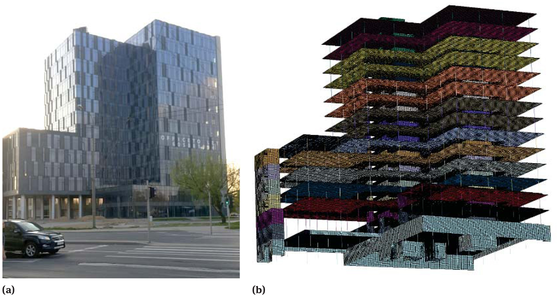
The analysed building: a) a perspective of the view structure, b) a 3D numerical model
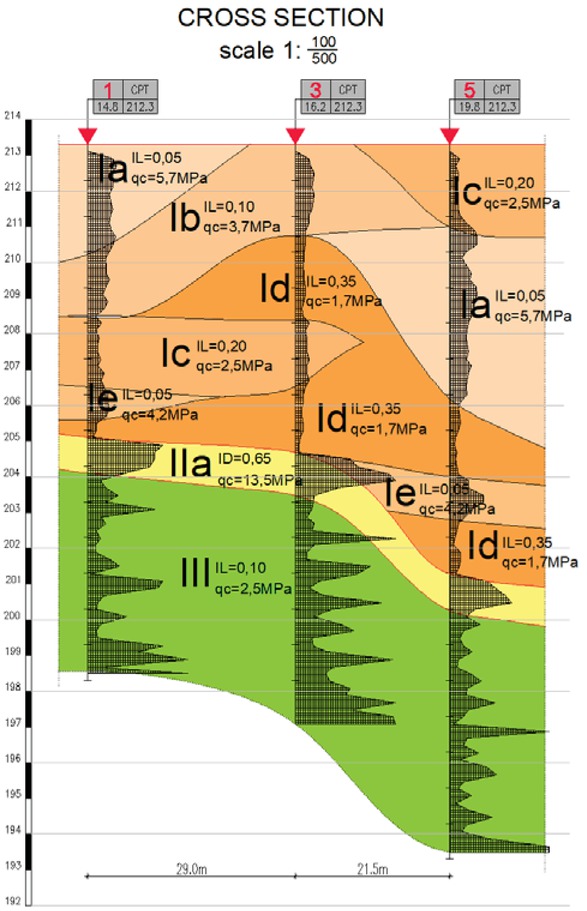
The representative geotechnical cross-section
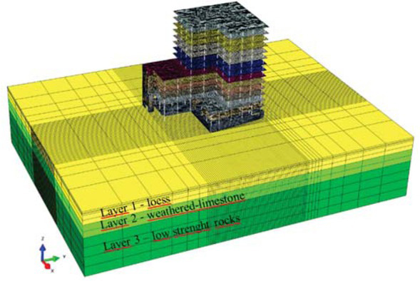
The view of the complete FEM “building–ground” model
Two Cam-Clay model parameter variants were assumed for the loess soil layer. The first variant, provisionally referred to as “EDO”, was based on the results of oedometer tests performed on samples with an undisturbed soil structure, taken from boreholes during construction. On the dependency charts e–ln(σ) (Figure 4) the lines of primary and secondary loading and the formulae describing the slope of these straight lines are presented. In the chart e is a void ratio, and σ is normal pressure. These charts were the basis for determining the initial parameters of the Cam-Clay model – λ and κ, where λ is the slope of the normal (virgin) consolidation line, while κ is the slope of unloading-reloading line.
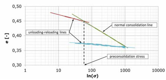
Oedometer-sample compression curves
In the calculations it was assumed that the soil was normally consolidated, and the preconsolidation stresses p0 corresponded to geostatic stresses. The slope of critical state lane in p-q space called as M parameter of the Cam-Clay model was calculated with the assumption of the internal friction angle φ = 35◦, based on an analysis of the tests of Lublin loess soils [13]. The void ratios e0 and e1 were determined from basic laboratory tests and consolidation charts.
In the second parameter variant, refered to as “CPT,” the parameters were estimated by combining the results of laboratory tests and CPT soundings, which were transformed into Cam Clay model parameters using the procedure described in [14]. Both the lithology and heterogeneity of the subsoil, identified by CPT soundings, were taken into account in the division into geotechnical layers. Afterwards, the mean cone resistance was calculated in respect of loesses as a weighted mean, where the thickness of the separated layer was taken as the weight. The mean value of cone resistance was qc = 3.27 MPa. On this basis and with the assumed coefficient αm = 6 the mean constrained modulus for the layer was determined as MCPT = 19.6 MPa [14]. This modulus was the basis for determining the slope of the primary consolidation line λ. The parameters of the Cam Clay model used for calculations for both these variants are listed in Table 1.
The parameters of loess layer for Cam-Clay model
| Variant | λ | κ | M | a0 | p0 | e1 | e0 |
|---|---|---|---|---|---|---|---|
| EDO | 0.0300 | 0.0042 | 1.495 | 28.1 | 108 | 0.561 | 0.421 |
| CPT | 0.0130 | 0.0042 | 1.495 | 32.6 | 108 | 0.584 | 0.523 |
Rocky subsoil is located in the deeper parts and its movements are limited to a very small range of deformations. For these layers the simplified model of Coulomb-Mohr was adopted and the parameters were derived from among other things, the following works [1, 9, 10, 15]. For the soil layers elastic properties were assigned with values similar to the initial deformation modulus. After the analysis of the literature data [16, 17] the angle of internal friction was assumed as φ = 40÷45◦, with a cohesion of c = 50÷2000 kPa. The value of the constrained modulus for rock layers was assumed as E = 2000 MPa for the lower zone of cracked carbonate rock (marl, opoka, gaize). For the upper zone – partially weathered – the modulus was estimated as E = 300 MPa with the use of literature data [10, 16] and on the basis of own research on the shear wave velocity Vs measured for the weathered layers in SDMT tests in Lublin.
3 Numerical analyses and results
In each of the calculation variants, successive floors were added in the calculation steps. In order to illustrate the calculation process Figure 5 presents the vertical displacements in selected calculation steps.
![Figure 5 Vertical displacements [m] in selected successive phases of construction](/document/doi/10.1515/eng-2020-0060/asset/graphic/j_eng-2020-0060_fig_005.jpg)
Vertical displacements [m] in selected successive phases of construction
Figure 6 shows the comparison of vertical displacements for two soil-parameter variants – EDO and CPT. The model with EDO parameters shows greater settlement than the CPT model. The maximum vertical displacement was 89.7 mm for the EDO model, and 51.7 mm for the CPT model. These are total values, from the start of the construction works, and should not be compared directly with the measured values, which are presented in relation to the reference measurement taken after constructing part of the structure. The displacement values in relation to the first geodetic measurement were 77.4 mm for the EDO parameters and 38.5 mm for the CPT parameters. The settlement determined with the EDO parameters significantly exceeded the actual settlement (22.0 mm), and the model with the CPT parameters was adopted for further analysis.
![Figure 6 Vertical displacements [m] in the building model with the body of the subsoil: a) EDO variant model, b) CPT variant model](/document/doi/10.1515/eng-2020-0060/asset/graphic/j_eng-2020-0060_fig_006.jpg)
Vertical displacements [m] in the building model with the body of the subsoil: a) EDO variant model, b) CPT variant model
The numerical calculations were compared to the actual settlement values. In subsequent calculation steps, the values of vertical displacements at the nodes corresponding to the location of benchmarks in the base slab were taken. The data and comparison to the measured values are listed in Table 2. The measured and calculated settlement values were compared directly and relative to the permissible settlement,whichwas assumed at 50 mm.The final comparison was made on averaged-out values. Some of the benchmarks were destroyed during the construction works.
A summary of vertical displacements in the successive calculation steps
| Benchmark | Settlement in calculation step [mm] | ||||||||||||
|---|---|---|---|---|---|---|---|---|---|---|---|---|---|
| Plate | KP | K1 | K2 | K3 | K4 | K5 | K6 | K78 | K910 | K1112 | K1314 | Finishing | |
| 6 | 0.0 | 0.4 | 1.3 | 2.2 | 3.0 | 3.9 | 4.8 | 5.9 | 8.8 | 12.2 | 15.6 | 19.2 | 29.1 |
| 7 | 0.0 | 1.5 | 2.3 | 3.7 | 5.0 | 6.4 | 7.8 | 9.5 | 12.9 | 16.5 | 20.0 | 23.8 | 34.3 |
| 8 | 0.0 | 2.5 | 3.9 | 5.2 | 6.3 | 7.4 | 8.4 | 9.6 | 12.8 | 16.6 | 20.7 | 24.8 | 36.0 |
| 9 | 0.0 | 2.5 | 3.8 | 5.3 | 6.6 | 8.0 | 9.4 | 11.2 | 15.6 | 20.2 | 24.8 | 29.7 | 40.9 |
| 11 | 0.0 | 0.5 | 1.6 | 2.5 | 3.3 | 4.0 | 4.7 | 5.5 | 7.2 | 9.7 | 12.5 | 15.3 | 24.8 |
| 12 | 0.0 | 0.9 | 1.7 | 2.3 | 3.0 | 3.6 | 4.2 | 4.8 | 6.4 | 8.5 | 10.7 | 13.1 | 20.0 |
| 13 | 0.0 | 1.9 | 2.7 | 4.0 | 5.0 | 5.9 | 6.9 | 7.9 | 10.0 | 12.4 | 14.9 | 17.6 | 26.2 |
| 14 | 0.0 | 2.2 | 3.2 | 4.3 | 5.0 | 5.6 | 6.2 | 6.9 | 8.6 | 10.6 | 12.8 | 15.1 | 22.6 |
| 15 | 0.0 | −1.4 | −1.3 | −1.2 | −1.1 | −1.0 | −1.0 | −0.9 | −0.7 | −0.4 | 0.0 | 0.4 | 2.1 |
| 16 | 0.0 | 0.7 | 1.6 | 3.3 | 4.8 | 6.3 | 7.9 | 9.7 | 10.1 | 10.5 | 10.8 | 11.3 | 15.8 |
| 17 | 0.0 | 0.0 | 0.2 | 1.6 | 3.0 | 4.4 | 5.8 | 7.2 | 7.1 | 6.9 | 6.8 | 6.6 | 11.1 |
| 18 | 0.0 | 2.8 | 4.1 | 5.5 | 6.6 | 7.7 | 8.7 | 10.1 | 13.7 | 17.7 | 21.7 | 26.0 | 36.4 |
| 19 | 0.0 | 2.6 | 4.0 | 5.4 | 6.8 | 8.2 | 9.6 | 11.5 | 16.3 | 21.4 | 26.4 | 31.8 | 43.7 |
| 20 | 0.0 | 2.3 | 3.6 | 4.9 | 6.2 | 7.4 | 8.6 | 10.3 | 14.5 | 19.3 | 24.0 | 28.9 | 40.8 |
| Average | 0.0 | 1.4 | 2.3 | 3.5 | 4.5 | 5.6 | 6.6 | 7.8 | 10.2 | 13.0 | 15.8 | 18.8 | 27.4 |
| Measured (average) | 0.0 | 2.2 | 2.2 | 2.3 | 3.3 | 3.3 | 3.3 | 3.5 | 5.5 | 6.2 | 6.7 | 7.5 | 17.2 (25.0)[*] |
| Error [mm] | 0.0 | 0.8 | −0.2 | −1.2 | −1.2 | −2.2 | −3.2 | −4.3 | −4.7 | −6.8 | −9.2 | −11.3 | 9.8 (2.4)[*] |
| Relative error [%] | 0.0 | 1.6 | −0.4 | −2.3 | −2.4 | −4.4 | −6.5 | −8.6 | −9.5 | −13.7 | −18.3 | −22.7 | 19.6 (4.8)[*] |
The chart of the displacements of the benchmarks prepared on the basis of the actual measurements indicates that the building settlement had not yet stabilised so, after the analysis of the literature data [18, 19] the final settlement was estimated by extrapolation of the results, which is shown in Figure 7. The chart shows the displacements of the benchmarks which remained until the last measurement, and the mean value of these measurements. The average final settlement was found to be approximately 25 mm with a maximum of 33 mm.
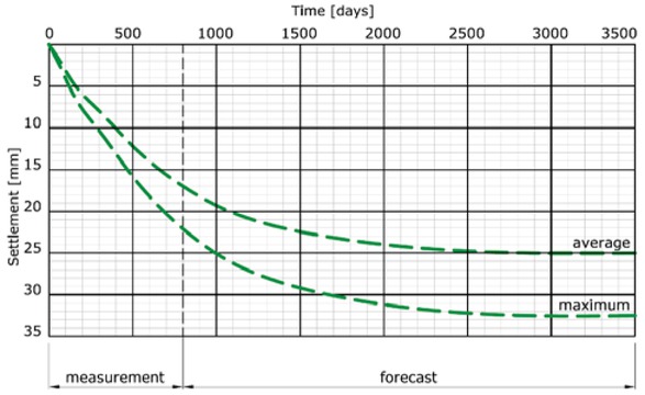
Forecast final settlement of the building
In the analysis of the displacement results presented in Table 2 it can be seen that the measured displacement values are higher than the calculated ones in the initial settlement phase alone. After crossing the calculation step KP, the calculated values exceeded the measured values. According to the author, it is caused primarily by spreading the actual settlement over time, which was not taken into account in the calculations. At this stage, the relative calculation error in relation to the value obtained in the last settlement measurement was less than 20%,which is not a very-significant error in the context of geotechnical calculations; moreover, the result of the calculations is on the safe side for the building. However, due to the fact that the actual settlement of the building is not final this error will decrease. If the author confirms the estimated final mean settlement value of 25 mm, the error will be less than 5%, which should be considered a very-good result.
In Figure 8 the displacement map of the base slab obtained from the calculations and that created on the basis of displacement measurements are compared. The values of displacements do not overlap, because the maps for calculations are given as final and the geodetic ones as the last measurement; however one should pay attention to the shape and arrangement of isolines, which substantially overlap with each other on both maps, which confirms the correctness of the calculations.
![Figure 8 Map of the base-slab settlement on the basis of: a) measurements of the real actual settlement [mm], b) calculations in ABAQUS [m]](/document/doi/10.1515/eng-2020-0060/asset/graphic/j_eng-2020-0060_fig_008.jpg)
Map of the base-slab settlement on the basis of: a) measurements of the real actual settlement [mm], b) calculations in ABAQUS [m]
To assess the impact of the subsoil work on structural elements, additional calculations were made with rigid supports under the base slab instead of the subsoil. Stresses in structural elements were compared for both calculations. In Figure 9 the minimum principal stresses are shown, while in Figure 10 the maximum ones are shown. The maps show increased stress zones. Significant differences can be seen primarily on the walls of underground floors. For rigid supports, these walls work as compressed. For a subsoil model defined with elastico-plastic behaviour, the bent base slab makes the walls work a bit as deep beam and the change in stress distribution is significant.
![Figure 9 Minimum principal stress [kPa]: a) in model with rigid support, b) in model with subsoil defined by elastico-plastic Cam Clay model](/document/doi/10.1515/eng-2020-0060/asset/graphic/j_eng-2020-0060_fig_009.jpg)
Minimum principal stress [kPa]: a) in model with rigid support, b) in model with subsoil defined by elastico-plastic Cam Clay model
![Figure 10 Maximum principal stress [kPa]: a) in model with rigid support, b) in model with subsoil defined by elastico-plastic Cam Clay model](/document/doi/10.1515/eng-2020-0060/asset/graphic/j_eng-2020-0060_fig_010.jpg)
Maximum principal stress [kPa]: a) in model with rigid support, b) in model with subsoil defined by elastico-plastic Cam Clay model
4 Conclusions
As a result of the numerical analyses the forecast settlement of the building was obtained, which was then compared with the geodetic measurements. At the time of the last geodetic measurement the settlement had not yet stabilised but the partial results indicate a high convergence of the calculation results with the actual behaviour of the building. In the case of loesses the Cam Clay model can be used to simulate the movement of the subsoil, whose parameters the author proposes to determine with tests performed using CPT soundings. A more-detailed analysis of the presented results can be found in [14].
References
[1] Chai J, Shen S, Ding W, Zhu H, Carter J. Numerical investigation of the failure of a building in Shanghai, China [Internet]. Comput Geotech. 2014;55(7):482–93.10.1016/j.compgeo.2013.10.001Suche in Google Scholar
[2] Grodecki M. Modelowanie numeryczne statyki ścianek szczelnych i szczelinowych. Politechnika Krakowska; 2007 [in Polish].Suche in Google Scholar
[3] Lechowicz Z, Kiziewicz D, Wrzesiński G. Ocena nośności podłoża w warunkach bez odpływu pod stopą fundamentową obciążoną mimośrodowo według Eurokodu 7. Acta Archit. 2013;12(3):51–60 [in Polish].Suche in Google Scholar
[4] Biały M. Zastosowanie modelu FC+MCC w analizie numerycznej współpracy chłodni kominowej z podłożem gruntowym. Czas Tech. 2008;3-Ś:21–9 [in Polish].Suche in Google Scholar
[5] Kowalska A. Analiza wpływu elementów niekonstrukcyjnych na charakterystyki dynamiczne budynków. Politechnika Krakowska; 2007 [in Polish].Suche in Google Scholar
[6] Mrozek D, Mrozek M, Fedorowicz J. The protection of masonry buildings in a mining area [Internet]. Procedia Eng. 2017;193:184–91. Available from: http://linkinghub.elsevier.com/retrieve/pii/S187770581732750910.1016/j.proeng.2017.06.202Suche in Google Scholar
[7] Mrozek D. Nieliniowa analiza numeryczna dynamicznej odpowiedzi uszkodzonych budynków. Politechnika Śląska w Gliwicach; 2010 [in Polish].Suche in Google Scholar
[8] Przewlocki J, Zielinska M. Analysis of the behavior of foundations of historical buildings [Internet]. Procedia Eng. 2016;161:362–7.10.1016/j.proeng.2016.08.575Suche in Google Scholar
[9] Comodromos EM, Papadopoulou MC, Konstantinidis GK. Effects from diaphragm wall installation to surrounding soil and adjacent buildings [Internet]. Comput Geotech. 2013;53:106–21.10.1016/j.compgeo.2013.05.003Suche in Google Scholar
[10] Ko J, Cho J, Jeong S. Nonlinear 3D interactive analysis of superstructure and piled raft foundation [Internet]. Eng Struct. 2017;143:204–18.10.1016/j.engstruct.2017.04.026Suche in Google Scholar
[11] Słowik L. Wpływ nachylenia terenu spowodowanego podziemną eksploatacją górniczą na wychylenie obiektów budowlanych. 2015 [in Polish].Suche in Google Scholar
[12] Simulia. Abaqus 6.9 User Manual. 2009;Suche in Google Scholar
[13] Nepelski K, Rudko M. Identyfikacja parametrów geotechnicznych lessów lubelskich na podstawie sondowań statycznych CPT. Przegląd Nauk Inżynieria i Kształtowanie Środowiska [Internet]. 2018;27(2):186–98. Available from: http://iks.pn.sggw.pl/PN80/A9/zeszyt80art9en.htmlhttps://doi.org/10.22630/PNIKS.2018.27.2.18 [in Polish].10.22630/PNIKS.2018.27.2.18Suche in Google Scholar
[14] Nepelski K. Numeryczne modelowanie pracy konstukcji posadowionej na lessowym podłożu gruntowym. Rozprawa doktorska. 2019 [in Polish].Suche in Google Scholar
[15] Szulborski K, Wysokiński L. Ocena współpracy konstrukcji z podłożem. Mat VIII Konf „Problemy rzeczoznawstwa budowlanego. Cedzyna; 2004 [in Polish].Suche in Google Scholar
[16] Paleczek W. Analiza korelacji wybranych parametrów geomechanicznych skał. Zesz Nauk Politech Częstochowskiej Bud. 2008;14:91–9 [in Polish].Suche in Google Scholar
[17] Pisarczyk S. Gruntoznawstwo inżynierskie. PWN; 2015.Suche in Google Scholar
[18] Hansbo S. Deformationer och sattiningar. Stockkholm: Liber Forlag; 1984.Suche in Google Scholar
[19] Lechowicz Z, Szymański A. Odkształcenia i stateczność nasypów na gruntach organicznych cz. I. Metodyka badań. SGGW Warszawa; 2002 [in Polish].Suche in Google Scholar
© 2020 K. Nepelski, published by De Gruyter
This work is licensed under the Creative Commons Attribution 4.0 International License.
Artikel in diesem Heft
- Regular Articles
- Fabrication of aluminium covetic casts under different voltages and amperages of direct current
- Inhibition effect of the synergistic properties of 4-methyl-norvalin and 2-methoxy-4-formylphenol on the electrochemical deterioration of P4 low carbon mold steel
- Logistic regression in modeling and assessment of transport services
- Design and development of ultra-light front and rear axle of experimental vehicle
- Enhancement of cured cement using environmental waste: particleboards incorporating nano slag
- Evaluating ERP System Merging Success In Chemical Companies: System Quality, Information Quality, And Service Quality
- Accuracy of boundary layer treatments at different Reynolds scales
- Evaluation of stabiliser material using a waste additive mixture
- Optimisation of stress distribution in a highly loaded radial-axial gas microturbine using FEM
- Analysis of modern approaches for the prediction of electric energy consumption
- Surface Hardening of Aluminium Alloy with Addition of Zinc Particles by Friction Stir Processing
- Development and refinement of the Variational Method based on Polynomial Solutions of Schrödinger Equation
- Comparison of two methods for determining Q95 reference flow in the mouth of the surface catchment basin of the Meia Ponte river, state of Goiás, Brazil
- Applying Intelligent Portfolio Management to the Evaluation of Stalled Construction Projects
- Disjoint Sum of Products by Orthogonalizing Difference-Building ⴱ
- The Development of Information System with Strategic Planning for Integrated System in the Indonesian Pharmaceutical Company
- Simulation for Design and Material Selection of a Deep Placement Fertilizer Applicator for Soybean Cultivation
- Modeling transportation routes of the pick-up system using location problem: a case study
- Pinless friction stir spot welding of aluminium alloy with copper interlayer
- Roof Geometry in Building Design
- Review Articles
- Silicon-Germanium Dioxide and Aluminum Indium Gallium Arsenide-Based Acoustic Optic Modulators
- RZ Line Coding Scheme With Direct Laser Modulation for Upgrading Optical Transmission Systems
- LOGI Conference 2019
- Autonomous vans - the planning process of transport tasks
- Drivers ’reaction time research in the conditions in the real traffic
- Design and evaluation of a new intersection model to minimize congestions using VISSIM software
- Mathematical approaches for improving the efficiency of railway transport
- An experimental analysis of the driver’s attention during train driving
- Risks associated with Logistics 4.0 and their minimization using Blockchain
- Service quality of the urban public transport companies and sustainable city logistics
- Charging electric cars as a way to increase the use of energy produced from RES
- The impact of the truck loads on the braking efficiency assessment
- Application of virtual and augmented reality in automotive
- Dispatching policy evaluation for transport of ready mixed concrete
- Use of mathematical models and computer software for analysis of traffic noise
- New developments on EDR (Event Data Recorder) for automated vehicles
- General Application of Multiple Criteria Decision Making Methods for Finding the Optimal Solution in City Logistics
- The influence of the cargo weight and its position on the braking characteristics of light commercial vehicles
- Modeling the Delivery Routes Carried out by Automated Guided Vehicles when Using the Specific Mathematical Optimization Method
- Modelling of the system “driver - automation - autonomous vehicle - road”
- Limitations of the effectiveness of Weigh in Motion systems
- Long-term urban traffic monitoring based on wireless multi-sensor network
- The issue of addressing the lack of parking spaces for road freight transport in cities - a case study
- Simulation of the Use of the Material Handling Equipment in the Operation Process
- The use of simulation modelling for determining the capacity of railway lines in the Czech conditions
- Proposals for Using the NFC Technology in Regional Passenger Transport in the Slovak Republic
- Optimisation of Transport Capacity of a Railway Siding Through Construction-Reconstruction Measures
- Proposal of Methodology to Calculate Necessary Number of Autonomous Trucks for Trolleys and Efficiency Evaluation
- Special Issue: Automation in Finland
- 5G Based Machine Remote Operation Development Utilizing Digital Twin
- On-line moisture content estimation of saw dust via machine vision
- Data analysis of a paste thickener
- Programming and control for skill-based robots
- Using Digital Twin Technology in Engineering Education – Course Concept to Explore Benefits and Barriers
- Intelligent methods for root cause analysis behind the center line deviation of the steel strip
- Engaging Building Automation Data Visualisation Using Building Information Modelling and Progressive Web Application
- Real-time measurement system for determining metal concentrations in water-intensive processes
- A tool for finding inclusion clusters in steel SEM specimens
- An overview of current safety requirements for autonomous machines – review of standards
- Expertise and Uncertainty Processing with Nonlinear Scaling and Fuzzy Systems for Automation
- Towards online adaptation of digital twins
- Special Issue: ICE-SEAM 2019
- Fatigue Strength Analysis of S34MnV Steel by Accelerated Staircase Test
- The Effect of Discharge Current and Pulse-On Time on Biocompatible Zr-based BMG Sinking-EDM
- Dynamic characteristic of partially debonded sandwich of ferry ro-ro’s car deck: a numerical modeling
- Vibration-based damage identification for ship sandwich plate using finite element method
- Investigation of post-weld heat treatment (T6) and welding orientation on the strength of TIG-welded AL6061
- The effect of nozzle hole diameter of 3D printing on porosity and tensile strength parts using polylactic acid material
- Investigation of Meshing Strategy on Mechanical Behaviour of Hip Stem Implant Design Using FEA
- The effect of multi-stage modification on the performance of Savonius water turbines under the horizontal axis condition
- Special Issue: Recent Advances in Civil Engineering
- The effects of various parameters on the strengths of adhesives layer in a lightweight floor system
- Analysis of reliability of compressed masonry structures
- Estimation of Sport Facilities by Means of Technical-Economic Indicator
- Integral bridge and culvert design, Designer’s experience
- A FEM analysis of the settlement of a tall building situated on loess subsoil
- Behaviour of steel sheeting connections with self-drilling screws under variable loading
- Resistance of plug & play N type RHS truss connections
- Comparison of strength and stiffness parameters of purlins with different cross-sections of profiles
- Bearing capacity of floating geosynthetic encased columns (GEC) determined on the basis of CPTU penetration tests
- The effect of the stress distribution of anchorage and stress in the textured layer on the durability of new anchorages
- Analysis of tender procedure phases parameters for railroad construction works
- Special Issue: Terotechnology 2019
- The Use of Statistical Functions for the Selection of Laser Texturing Parameters
- Properties of Laser Additive Deposited Metallic Powder of Inconel 625
- Numerical Simulation of Laser Welding Dissimilar Low Carbon and Austenitic Steel Joint
- Assessment of Mechanical and Tribological Properties of Diamond-Like Carbon Coatings on the Ti13Nb13Zr Alloy
- Characteristics of selected measures of stress triaxiality near the crack tip for 145Cr6 steel - 3D issues for stationary cracks
- Assessment of technical risk in maintenance and improvement of a manufacturing process
- Experimental studies on the possibility of using a pulsed laser for spot welding of thin metallic foils
- Angular position control system of pneumatic artificial muscles
- The properties of lubricated friction pairs with diamond-like carbon coatings
- Effect of laser beam trajectory on pocket geometry in laser micromachining
- Special Issue: Annual Engineering and Vocational Education Conference
- The Employability Skills Needed To Face the Demands of Work in the Future: Systematic Literature Reviews
- Enhancing Higher-Order Thinking Skills in Vocational Education through Scaffolding-Problem Based Learning
- Technology-Integrated Project-Based Learning for Pre-Service Teacher Education: A Systematic Literature Review
- A Study on Water Absorption and Mechanical Properties in Epoxy-Bamboo Laminate Composite with Varying Immersion Temperatures
- Enhancing Students’ Ability in Learning Process of Programming Language using Adaptive Learning Systems: A Literature Review
- Topical Issue on Mathematical Modelling in Applied Sciences, III
- An innovative learning approach for solar power forecasting using genetic algorithm and artificial neural network
- Hands-on Learning In STEM: Revisiting Educational Robotics as a Learning Style Precursor