Cloud computing-based framework for heart disease classification using quantum machine learning approach
-
Huda Ghazi Enad


Abstract
Accurate early identification and treatment of cardiovascular diseases can prevent heart failure problems and reduce mortality rates. This study aims to use quantum learning to predict heart problems to increase the accuracy of traditional prediction and classification methods. Machine learning (ML) and deep learning (DL) techniques need quantum learning to quickly and accurately analyze massive volumes of complex data. With quantum computing, the suggested DL and ML algorithms can change their predictions on the basis of changes in the dataset. This approach could help with the early and accurate detection of chronic diseases. The Cleveland heart disease dataset is undergoing preliminary processing to validate missing values to increase the precision rate and prevent incorrect forecasts. This study examined the feasibility of employing and deploying a quantum ML (QML) framework via cloud computing to categorize cardiac conditions. The research was divided into four sections. First, the principal component analysis was used to preprocess the Cleveland dataset, recursive feature elimination was used to select features, and min–max normalization was used to give the dataset a high-dimensional value. Second, we compared traditional classifiers, such as support vector machine (SVM) and artificial neural network, with the quantum approach to verify the quantum approach’s efficiency. Third, we examined two unique QML classification methods: quantum neural networks (QNNs) and quantum SVM (QSVM). Fourth, bagging-QSVM was developed and deployed as an ensemble learning model. Experimental results using the QNN show an accuracy of 77%, a precision of 76%, a recall of 73%, and an F1 score of 75%. With an accuracy of 85%, a precision of 79%, a recall of 90%, and an F1-score of 84%, the QSVM method demonstrated a much better performance than the QNN. Particularly, the Bagging_QSVM model exhibited an outstanding performance, with a flawless score of 100% across all critical performance measures. The study shows that the bagging method for ensemble learning is a solid way of increasing the accuracy of quantum method predictions.
1 Introduction
Diseases of the heart and blood vessels, sometimes known as cardiovascular diseases (CVDs), are a leading cause of death in the United States [1]. Approximately 17.9 million fatalities are recorded per year, or 32% of all deaths are attributed to CVDs each year, as reported by the World Health Organization (WHO) [2]. High blood lipid levels, obesity, high blood glucose levels, and high blood pressure are all risk factors for these diseases [3]. Heart disease (HD) is among the biggest threats to global community health. The widespread occurrence of HD and the accompanying rise in the mortality rate threaten human safety. Thus, the early diagnosis of cardiac disease by identifiable physical markers is essential for impeding disease’s progression and mitigating its long-term repercussions. Preventative approaches for HD have been a study focus for quite some time [4]. Furthermore, several studies have used machine learning (ML) methods in the attempt to forecast the chances of developing HD. Studies have embraced ML methodologies in several medical domains to improve and optimize medical decision-making. ML techniques are typically employed to automatically find patterns in a dataset without any further human input. However, traditional ML methods may be improved for better outcomes and increased reliability [5,6,7]. Models utilize a wide range of ML methods, including ensemble learning, which has been found to boost model performance for predicting cardiovascular illnesses [8,9,10]. As an alternative to traditional ML methods, quantum computing may offer a more effective framework. Quantum ML (QML) is a young but rapidly developing topic of research. This research aimed to design a model based on an existing QML model to determine whether ensemble learning and QML can help predict the risk of CVDs. Given that ML techniques can provide reliable answers for predicting the existence of cardiac disease, the study used both conventional and cutting-edge QML techniques.
Early identification helps substantially reduce the mortality from HD, which is regarded as one of the major causes of death. Traditional prediction methods are complex because of the complexity of data and the correlations that arise during the process. Conventional ML and deep learning (DL) methods [11] have used medical records from the past to make predictions about the condition of patients. A study by Gupta et al. [12] shows how support vector machine (SVM), Naive–Bayes, and decision tree (DT) are three types of supervised learning algorithms that are used on HD data to make highly accurate predictions. Another method used the African HD dataset, which has 462 cases, and utilized intelligent systems to perform a 10-fold cross-validation [13]. Using smart devices to monitor patients in real time can slow disease progression. However, the need for good data streaming and analysis capabilities with massive volumes of real-time data hampers proper and prompt diagnosis. The method suggested in another study [14] demonstrates that electrocardiogram (ECG) data can be accessed through a monitoring method that works over 5G using the Flink-based streaming of information extraction framework [15]. Long short-term memory and convolutional neural networks (CNNs) have also been helpful in automatic patient health prediction [16].
To improve the precision and effectiveness of HD classification, this study aims to create a system that employs QML inside a cloud computing setting. This approach intends to increase the accuracy and speed with which various cardiac problems or risk factors may be identified by incorporating quantum computing ideas into ML algorithms. The framework intends to manage lengthy computations and massive datasets, ultimately enhancing HD prediction models using cloud infrastructure’s scalability and processing power. The ultimate aim is to improve healthcare diagnostics and mitigation in cardiac health monitoring by achieving precise diagnoses, providing highly trustworthy risk evaluations, and maybe enabling real-time or near-real-time classification of instances. The proposed technique is appropriate for data classification and prediction and has broad applications in quantum computing. The present study aims to effectively predict CVDs while addressing the issues encountered in previous research. The current study has the following contributions:
To develop a cloud-based system for classifying HDs that can monitor health data from remote users and identify HD classifications.
Several preprocessing methods, comprising feature selection, feature extraction, and normalization, are used to prepare the data for analysis.
To investigate the potential of QML models by comparing their performance to that of conventional ML classifiers like artificial neural network (ANN) and SVM. Then, we use quantum neural network (QNN) and quantum SVM (QSVM), two different quantum ML classifiers. This stage aims to determine the most efficient QML approach for the provided dataset.
To develop, implement, and evaluate a brand-new ML model (bagging-QSVM-based bagging ensemble learning method). The SVM-recursive feature elimination (RFE) method is used to calculate and demonstrate each feature’s relevance and personal involvement in predictions made by the model, which sets this research apart from others.
To compare the precision, accuracy, recall, and f-score of several effective classification methods to demonstrate the efficacy of the proposed approach.
The structure of this study incorporates several perspectives. Section 2 presents a comprehensive assessment of approaches to classifying HD. Section 3 proposes QML for HD, analyzes the bagging-QSVM model, and discusses the mathematical foundations of QML and its particular relevance to the HD classification. In Section 4, the results from using the bagging-QSVM model are presented, discussed, and compared with those of current approaches. Finally, the study’s contributions, significant consequences, and implications are summarized in Section 5.
2 Related works
Classification algorithms based on ML have several uses and are a valuable tool for solving complex problems. Healthcare is widely acknowledged to be a field where ML applications abound, providing possibilities for improving a wide range of clinical judgments. Researchers have prioritized HD research over other healthcare problems using revolutionary ML approaches. Ensemble learning plays a pivotal role in significantly enhancing the overall performance of ML models. Ensemble learning has been used successfully in several previous studies with a wide range of approaches for improved diagnostic skills to increase the precision of HD prediction.
The quantum particle swarm optimization (QPSO)-SVM model exhibits the highest degree of accuracy in the prognosis of cardiac ailments, achieving 96.31% on the Cleveland Heart Dataset. Moreover, an investigation revealed that the QPSO-SVM model outperforms other modern prognostic models in terms of precision (94.23%), sensitivity (96.13%), F1 score (0.95%), and specificity (93.56%). The QPSO-SVM model, which is an example of ML, utilizes QPSO to adapt the optimal SVM parameter for the precise anticipation of HD [17]. Future implementations for the prognosis of cardiac diseases should integrate various strategies to improve the speed and accuracy of detection for real-time application. A study posits that the proposed approach, which employs instance-based QML and DL methods, surpasses existing classification methods in terms of accurate prediction and cost-effective computational time. The accuracy of instance-based quantum DL is 98%, and that of instance-based quantum ML is 83.6%. In addition, the study revealed that the use of quantum-based DL and ML enhances system performance by reducing the computational time [18].
The utilization of the quantum paradigm exhibits a potential to expedite the process of K-means clustering. In the conducted study, the quantum K-means clustering technique was employed to identify instances of HD by applying a quantum circuit approach to the HD dataset. The research findings indicate that the quantum mechanical K-means clustering algorithm operates at a time complexity of O(LNK), which is notably faster than the traditional K-means clustering technique with a time complexity of O(LNpK). Furthermore, a comparative analysis was performed between quantum and classical processing to assess their performance metrics [19]. Quantum methodologies, such as QNN and hybrid random forest QNN, are highly suitable for the early prediction of cardiac diseases. In the aforementioned study, these quantum ML methods were employed for classification purposes on the Cleveland and Statlog datasets, resulting in reported areas under the curve values of 96.43 and 97.78%, respectively [20]. The limitations imposed by the study’s resources affected the full utilization of the entire dataset. As per the study findings, the implementation of quantitative structure-activity relationship machine learning (QML) techniques yielded a predictive accuracy of 84.64% for HD.
The study also posits that QML approaches demonstrate competence in analyzing medical signal data. For classification purposes, QNN, quantum means (Q-means), and quantum K-nearest neighbors (Q-KNN) were used. Consequently, the implementation of quantum ML classifiers may enhance early diagnosis and risk prediction in healthcare, particularly in HD. Various classifiers, such as the variational quantum classifier (VQC), QSVM, and QNN, and traditional ML techniques, including ANN, SVM, and the Shapley additive explanations (SHAP) framework, were employed. These classifiers were utilized in the classification of the Cleveland HD dataset. The study underscores the potential of QML in the healthcare sector; however, it also acknowledges the challenges associated with its application, primarily due to the lack of discourse surrounding computing requirements and limitations in research, which may impede its widespread adoption in healthcare environments. Further research endeavors are necessary to address these challenges and develop highly precise and efficient QML models for healthcare applications. The main limitation of the study stems from the utilization of small data samples in relation to a limited number of bits. The study used the quantum version of a fully CNN (FCQ-CNN) and SVM with RFE for dimension reduction to reach an excellent testing accuracy of 84.6% across all instances for heart datasets [21]. The summary of related works on HD diagnosis using QML is presented in Table 1.
Summary on related works on HD diagnosis using QML
| Author/Year | Dataset | Method | Strengths | Limitations |
|---|---|---|---|---|
| Elsedimy et al. 2023 [17] | Cleveland HD | QPSO | According to the Cleveland Heart Dataset, the suggested QPSO-SVM model has the highest percentage of accuracy (96.31%) in predicting HDs. | The QPSO-SVM model outperformed other models in heart disease prediction accuracy, F1 score, sensitivity, specificity, and precision using the Cleveland heart data set. |
| Alsubai et al. 2023 [18] | Cleveland HD | SVM, DT, and RF used for classification – instance-based quantum ML and DL methods used | In terms of precise prediction and economical computing time, the suggested approach performs better than existing classification methods. System performance is enhanced by quantum-based ML and DL, which lower computational found to be 98 and 83.6%, respectively. | Future implementations should combine several strategies for improved speed with early detection for real-time implementation. |
| Kavitha and Kaulgud 2022 [19] | HD dataset | Quantum K-means clustering | Quantum paradigm can speed up K-means clustering. Comparative analysis between quantum and classical processing. | Due to qubit coherence times and quantum noise, quantum computers are not able to answer problems with a tolerable degree of precision. |
| Heidari and Hellstern 2022 [20] | Cleveland and Statlog | QNN and hybrid random forest QNN | For the Cleveland and Statlog datasets, respectively, an area under the curve of 96.43 and 97.78% indicates that quantum approaches are better suitable for early cardiac disease prediction. | Due to the overfitting and high computational cost of QNN, overcoming problems related to incorrect tree depth and number selection. |
| Ozpolat and Karabatak 2023 [21] | Ningbo People’s and Shaoxing and Chapman University | Q-means, Q-KNN, and QNN | QML achieved 84.64% accuracy. QML techniques perform satisfactorily with signal data used in healthcare. | Limitations prevented the use of the complete dataset. Lack of available funds hampered the research. |
| Abdusalam et al. 2023 [9] | Cleveland HD | QNN, VQC, QSVM, traditional ML techniques like SHAP, ANN, and SVM | According to the study, QML methods might improve healthcare’s early diagnosis and risk prediction, particularly for HD. | The QML has potential in various sectors, but its application in healthcare remains challenging due to the lack of discussion on computing needs and constraints in research, potentially hindering its widespread use in healthcare environments. |
| Ullah et al. 2022 [22] | Electronic Health Records (EHR) by Basurto Hospital of the Basque Country | FCQ-CNN | FCQ-CNN considerably beat both conventional models utilizing the same training parameters and data sets. Completed all cardiovascular dataset tests with an unprecedented 84.6% accuracy. | The key disadvantage of this research is that it relied on very short data samples due to the limited number of bits used. |
| SVM along with RFE for dimension reduction |
Previous research reviews have used many intelligent prediction approaches with artificial intelligence (AI)-based classifiers to diagnose HD accurately using health-related data from medical databases. After reviewing the current literature, we compiled the following list of the most often encountered problems with prediction validation. Predictions of cardiac issues have been made using practical feature selection algorithms like the SVM and gradient boosting trees. These algorithms may be used with classifiers to increase prediction accuracy and gain resilience. Therefore, research on other aspects of nutrition and clinical predictor factors can aid in precise diagnosis. Predictability improvements may be achieved by employing quantum-based learning to rectify the imbalance observed between the positive and negative classifications in comparable medical datasets. The proposed approach has several potential uses in quantum computing and is well suited for data prediction and categorization. In light of the problems with earlier studies, the current investigation seeks to improve CVD prediction.
3 Proposed QML for HD diagnosis
To anticipate cardiac disease in patients, the proposed classification approach combines quantum-based learning with ML to identify shifts in health data from a dataset. To slow the disease’s spread and ensure that the right therapy is administered, the afflicted patient must be identified and placed in a specific category. The mortality rate is the primary target of the suggested strategy, which aims to reduce it through early diagnosis. Prediction accuracy has been an issue in previous research; the proposed model is being developed to improve performance by applying instance-based quantum ML methods. Figure 1 is a schematic of the model’s architecture. The figure provides an overview of the proposed prediction mechanism operation, which is broken down into the preprocessing and classification stages. The Cleveland HD dataset is used as the input for the proposed analysis. Patient health-related test results containing various predictive variables serve as the database’s input data. The data collected is preprocessed by eliminating any gaps in the information by filling in missing values and simplifying the data structure through dimensionality reduction. The next step is a two-stage classification procedure, after which the input data are separated into the training and test sets. In the first step, disease prediction is carried out independently using three different classifiers: a QNN, a QSVM, and a bagging-QSVM. The suggested instance-based quantum ML method for evaluating input data is used to execute the second step of the computation. By using the relationship between features, the method accurately determines patterns. Compared with conventional categorization methods, the suggested quantum model shows considerable improvements in precision and efficiency.
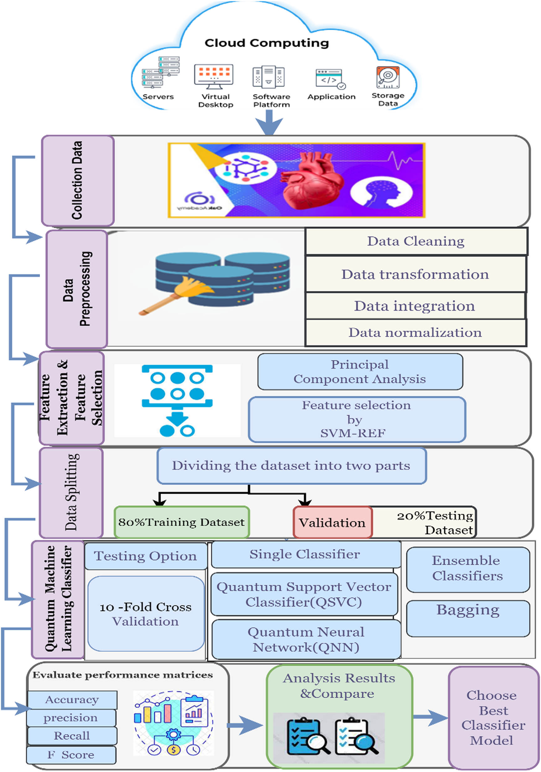
Proposed quantum ML for enhancing HD diagnosis.
This research aims to examine the feasibility of using quantum ML algorithms for HD diagnosis. The study is divided into four parts. First, the Cleveland dataset is preprocessed using several techniques, such as RFE to choose which features to use, principal component analysis (PCA) to extract these features, and min–max normalization. Second, quantum classifiers are compared with their conventional counterparts such as ANN and SVM. Third, QNN and quantum support vector machine (QSVM), which are two types of quantum ML classifiers, are examined. Finally, a QSVM-based bagging ensemble learning approach (i.e., bagging-QSVM) is developed and applied.
3.1 Cloud-based HD classification model
The present study suggests the development of a cloud-based system for classifying HDs and that can monitor health data from remote users and identify their HD category. The technology is sufficiently adaptable to support the diagnosis and classification of a wide range of disorders when applied to the consumer health data stored on cloud servers. Nonetheless, we primarily focused on a single instance of application, which included classifying the illness as either “normal” or “abnormal.” Figure 1 displays the general layout of the proposed architecture. In the architecture, patients visit a rural healthcare facility, where a practitioner collects data via wearable devices, performs imaging tests and medical history assessments, conducts surveys, obtains electronic records of health, and then transmits all information to a doctor, who then uploads it to a cloud platform for analysis.
3.2 Dataset collected
The HD dataset sourced from Kaggle is as a comprehensive compilation of HD-related data. The dataset merges information from five distinct datasets into a unified dataset. This merger extends across 12 common features, making it the most extensive HD dataset available for research purposes [23]. The five constituent datasets utilized for this are the Cleveland, Hungarian, Switzerland, Long Beach VA, and Statlog (Heart) datasets [24]. These datasets include male and female patients, resulting in a total of 1,190 records. Among these records are 11 distinctive features and a single target variable. The dataset accounts for 629 instances of HD and 561 instances of normal cardiac health. The age range of the patients included in the dataset is 57–60 years. Importantly, this dataset does not have any missing values. This dataset comprises a diverse set of features, incorporating six nominal and five numeric variables. For a comprehensive understanding of the dataset’s attributes, their description and that of the features included in the dataset on HD are presented in Table 2.
| Feature name | Data type | Description |
|---|---|---|
| Sex | Nominal | Male (−1), female (−0), or unsure () |
| Age | Numerical | Years of age of patients |
| Cholesterol | Numerical | Mean milligrams per deciliter of serum cholesterol |
| Fasting blood sugar | Nominal | If the fasting blood sugar is over 120 mg/dl, that is 1, and if it is below that, it is 0 |
| Chest pain type | Nominal | The patient’s chest discomfort is classified as either (1) typical, (2) typical angina, (3) nonanginal pain, or (4) asymptomatic |
| Resting bp s | Numerical | Resting blood pressure measured in millimeters of mercury |
| Resting ECG | Numerical | Three values are used to indicate the results of a resting ECG. 0: normal ST-T wave abnormality; 1: left ventricular hypertrophy |
| Exercise angina | Nominal | Exercise-related angina with 0 for NO and 1 for YES |
| Max heart rate | Numerical | Determined heart rate accomplished |
| ST slope | Nominal | Slope of the ST segment during maximal exercise 0 = typical sloping up (1), level (2), or sloping down (3) |
| Old peak | Numerical | Reduced mood after exercise compared to being at rest |
| Target | Normal | The goal variable is whether the patient has HD, where 1 indicates high risk and 0 indicates low risk |
3.3 Data preprocessing
In the preparation of the HD classification dataset, denoted as “Cleveland_statlog_Hungary,” several critical data preprocessing steps were employed to ensure data quality and enhance its suitability for classification tasks. The following primary processes were included.
3.3.1 Data cleaning
Data cleaning is a fundamental step that involves a meticulous examination of the dataset for any anomalies, such as missing values, outliers, or errors. When identified, outliers and errors are either rectified or removed, while missing values are imputed or excluded from the dataset. Notably, the comprehensive dataset from the merged Cleveland, Statlog, Hungary, Switzerland, and Long Beach datasets has no missing variables. Consequently, the focus of data pretreatment for classification shifted toward techniques such as feature engineering, dimensionality reduction, and data transformation for enhancing the performance of classification models. However, the statistical importance of the model analysis findings may be diminished due to missing values. For accurate and reliable analysis, missing values should be properly mitigated during data preparation. One duplicate row from 303 in the Cleveland dataset was modified and eliminated. Consequently, 302 distinct cases were obtained: 164 matched patients with HD and 138 matched patients without HD. We found all the values in Statlog. In addition, 272 identical occurrences were identified, leading to the removal of duplicate instances. Of these, 508 instances correspond to individuals with HD, while 410 instances represent those without HD.
3.3.2 Data integration
Integrating data that have been cleansed from many sources.
3.3.3 Data transformation
The data are transformed using the appropriate techniques. When specific data attributes have huge input values that are incompatible with other features, the learning performance might be poor. Thus, record research was carried out to visually study and select links to suit various features. This approach is achieved through one-warm encoding. One-hot encoding is possible with the available datasets when capabilities are combined with cp, thal, and slope. Before they are integrated with the original data sets, these three capabilities are subdivided into cp_0 to cp_3, thal_0 to thal_3, and slope_0 to slope_2. Before further processing, the data are scaled based on the statistical analysis results.
3.3.4 Data normalization
“Standardization” and “normalization” are two crucial methods of the feature scaling process. We normalized the data by taking the range of distributional changes and removing the mean and dividing it by the standard deviation. Centering is the process of eliminating the mean from data values, while scaling is the practice of dividing each data point by the standard deviation. The existence of outliers is preserved by standardization, making the final algorithm more resistant to outside effects than one that has not been standardized. Equations (1)–(3) can be used to standardize a given value.
Here, x is the original value, μ is the mean of the dataset, σ is the standard deviation, and x′ is the standardized value.
In this equation, the summation (∑) is taken over the range of N, and the mean (μ) is calculated by dividing the sum of all the values in the dataset (XN) by the total number of values (N). Mean is a measure of central tendency that represents the average value of a dataset, and it is used in various statistical analyses to compare the distribution of values in different datasets.
Standard deviation (σ) is a statistical measure used in various analyses, such as hypothesis testing and confidence interval estimation. This measure is calculated by dividing the squared differences between each value in the dataset and the mean by the total number of values. Normalization ensures that all characteristics have an equivalent magnitude, which is beneficial for data distributions that deviate from the Gaussian model. Normalization equation (4) is essential in preparing the data for min–max scaling.
Here, the values of
3.4 Feature extraction
Feature extraction is a significant stage in HD classification because it helps identify the most relevant features that can be utilized to train ML methods. Some feature extraction methods are used in HD classification such as the PCA technique, and it is a powerful tool utilized in ML to identify the most influential factors contributing to HD prediction. By reducing the dataset complexity, PCA enhances the overall performance of ML techniques. Essentially, PCA is a feature extraction technique that identifies the primary components within the data and uses them to transform its underlying structure.
PCA relies on a series of X-unit vectors, each of which represents the orientation of the line that provides the best match. After the first X1 components, all the others are perpendicular to each other. The first PC represents the axis along which data’s anticipated variance is maximized. By contrast, the data projections’ variance reaches the maximum in a path perpendicular to the initial X1 main components. PCA is a well-liked method for simplifying data by identifying its key drivers of variance. This method may be used for predictive modeling and exploratory data analysis. A lower-dimensional data collection can be constructed while keeping as much variance as possible by mapping every information point to only the first few major components. With PCA, a long list of variables can be shortened to a manageable subset that still accounts for the bulk of the original set. Overall, PCA is a potent technique that is extensively utilized because of its ability to improve the efficiency of ML algorithms. Based on the findings, PCA is computed as follows:
Standardizations: The continuous beginning variables are spread out such that they all have an equal impact on the study. The average and standard deviation for each factor are determined, and standardized data may be expressed as equation (5) by subtracting the mean from every parameter of the standard deviation.
(5)Here, µ = {µ1, µ2, … µm} represents the mean of the independent features, while σ = {σ 1, σ 2, … σ m } represents the standard deviation of the independent features. Z denotes the z-score, x denotes the original value, μ denotes the mean of the dataset, and σ denotes the standard deviation of the dataset. The z-score serves as a measure of the number of standard deviations of a value from the mean. A positive z-score indicates that the value exceeds the mean, and a negative z-score suggests that the value falls below the mean. The z-score proves valuable in statistical analyses, such as hypothesis testing and confidence interval estimation, because it enables the comparison of values from disparate datasets that may possess different means and standard deviations.
Covariance matrix calculation: The covariance matrix is calculated to identify the correlations between variables. The covariance matrix is calculated as follows:
where C is the covariance matrix, n is the number of observations, and X is the standardized data matrix. The eigenvalues and the eigenvectors are calculated. The equation used to calculate the covariance matrix of a dataset is a measure of the relationship between variables in a dataset. The equation measures how much the variables in the dataset are related to each other and helps in identifying the direction of the highest variance, which can be useful in PCA and other dimensionality reduction techniques to calculate the eigenvalues and eigenvectors of the covariance matrix following these steps:
The covariance matrix (C) is calculated using equation (6).
The eigenvalues (λ) and eigenvectors (v) of the covariance matrix (C) are determined using appropriate numerical methods such as QR decomposition or singular value decomposition.
The most minor and most significant values of that feature in the collection data are determined. The covariance matrix’s eigenvectors and eigenvalues are determined. Each eigenvector is a direction in which the data change remarkably, and its corresponding eigenvalue is the magnitude of that eigenvector’s fluctuation. The eigenvectors and the eigenvalues can be calculated using the following equation:
(7)where v is the eigenvector, λ is the eigenvalue, and C is the covariance matrix. The relationship between the eigenvector and eigenvalue of the covariance matrix is a pivotal concept in the examination of multivariate data and linear transformations.
The primary components and the eigenvectors with the largest eigenvalues are selected. The original data are transformed into a lower-dimensional space using PCA, where the immediate members stand in for the directions along which the data fluctuate the most.
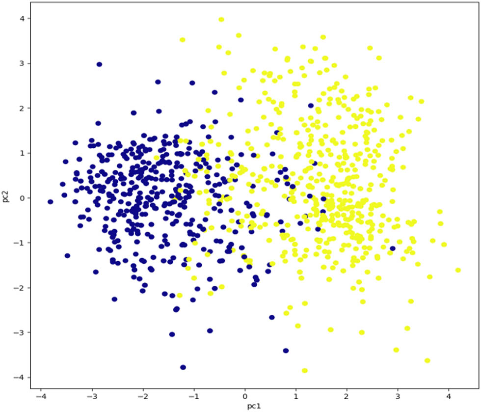
Visualization of results: The results are visualized using a scatter plot. A scatter plot of the data along the first and second main components of interest (x-axis and y-axis, respectively) is generated. Figure 2 shows that each point’s hue reflects a different dependent variable.
A 3D scatter plot of statistics inside the predominant thing space is generated. This form of plot is beneficial for visualizing records with three dimensions. The x-axis in Figure 3 represents the most essential aspect, the y-axis represents the second most important, and the z-axis is the 0.33 most important. The identification of patterns or connections in the statistics may be facilitated by the correspondence of each factor’s color to the variable of interest.
Visualization of results.
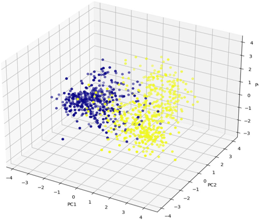
3D data visualization.
3.5 Feature selection
Selecting the most important input variables or features from a huge dataset is an essential part of ML. Reducing the data’s dimensionality in this manner can improve the performance of prediction models. With only the most pertinent details included, the model can zero in on what is essential in determining the outcome. Overfitting, which occurs when a model is extremely complicated and catches noise rather than underlying patterns, may also be avoided in this way. Different approaches are used for selecting features; the approach is dependent on the dataset and the current situation. A strong technique utilized in feature selection is the SVM-RFE approach, which employs SVM for evaluating features based on nonlinear kernels and for survival analysis. Figure 4 indicates that this approach aids in improving a classifier’s performance by selecting the most important features and discarding the rest.
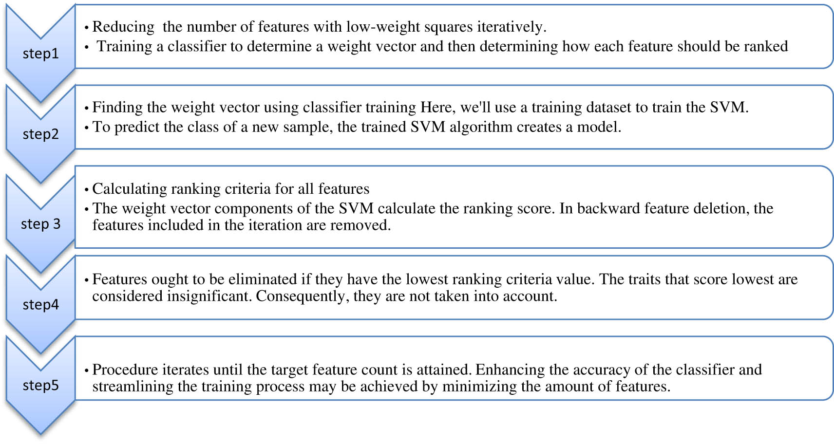
SVM-RFE steps.
The SVM-RFE technique is often used in disciplines such as ML and data mining. Users can boost the precision of their models for classification and hence the quality of their findings by employing this approach. To maximize a predictive model’s efficacy, the role that feature selection plays in ML must be appreciated. The following equation describes the SVM-RFE algorithm:
In this equation, w represents the weight vector, b is the bias term, C is the regularization parameter, and y_i is the dependent variable. The SVM-RFE method is an iterative algorithm that works backward from an initial set of features. In each round, the method fits a simple linear SVM and ranks the features based on their importance. The process is repeated until a feature-sorted list is obtained. Through SVM training using the feature subsets of the sorted list and evaluating the subsets using cross-validation, the optimal feature subsets can be identified. The SVM-RFE method consists of the steps presented in Figure 4.
3.5.1 Feature scaling
To standardize and scale the data, we use Standard Scaler and Min-MaxScaler. When the input variables have different scales or units, the Standard Scaler function normalizes the data by subtracting the mean and scaling to the unit variance. For each feature, Standard Scaler sets the mean to 0 and the standard deviation to 1. The “ca,” “cp,” “old peak,” “thal,” “exang,” and “slope” characteristics are scaled using this method.
3.5.2 Min-MaxScaler
Data may be scaled to a range between 0 and 1 using Min-MaxScaler. It shines when the input variables do not follow a Gaussian distribution and have varying ranges. Using Min-MaxScaler ensures the uniformity of features in size. To adjust the size of the features that have already been normalized, we use Min-MaxScaler.
The dataset is divided into the training and testing groups, with the training dataset as the basis for training ML techniques, while the testing dataset is designated for model performance assessment. The major focus of this section is the testing of the model’s performance on new information. A training set and a testing set (80 and 20% of the dataset, respectively) are created to begin the process.
3.6 Data splitting
Data splitting is a fundamental strategy in assessing ML algorithms. Overfitting may be avoided by splitting the dataset into training and testing sets, generating an accurate testing set, simulating the model’s behavior on simulated data, and assessing the results. Typically, 80% of the data is used for training, while 20% is used for testing. By using this proportion, the dataset would generate a training set with 952 records and a testing set with 238 records [2]. Figure 5 illustrates how the separation of training and testing datasets facilitates the training and assessment of different ML classifiers.
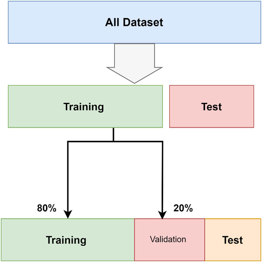
Split the dataset.
3.7 Classification stage
The study demonstrates the contribution of ML classification algorithms, including the ANN, SVM, QNN, QSVM, and bagging applied to QSVM, to the overall findings of the research. Following the dataset preparation process described in the previous two sections, ML techniques and quantum ML were used to implement categorization algorithms. The Scikit-Learn package must be utilized in the development of ML algorithms, and the Qiskit package uses QML. Regression, classification, and clustering are just a few of the ML algorithms included in the library, which is quite important in this field. The proposed system is implemented using a few of the functions offered by this library. The proposed system uses many Python libraries, including Google, in its implementation.
Colab: This library is used for the free Jupyter Notebook environment on Google Cloud servers known as Colab Notebooks.
NumPy library: This library is used for computing numerical data.
Pandas is a library for analyzing and manipulating data.
Matplotlib: This library is for making graphs, plots, and charts.
Seaborn: This is a matplotlib-based data visualization package.
Cv2: OpenCV is a well-known library for programming in real-time computer vision.
The Python library file system is the OS.
3.7.1 SVMs
SVM is a discriminative model because it fits a hyperplane that divides two classes. It is an approach to supervised ML that may be applied to issues related to regression and classification. It depicts a hyperplane, that is, a line that divides a plane in two, keeping and separating the multiple categories of data on either side for each class in a 2D environment. The SVM produces the hyperplane in the test data, which was built using the training data. The coordinates of each data point serve as the basis for the support vectors. This approach is mainly used to address classification issues. The method seeks out the hyperplane that minimizes the classification error while maximizing the margin. The efficiency relies on the specifications of the selected kernel and the soft margin setting. A quadratic problem of optimization may be used to describe the SVM method. Among the many kernelized learning algorithms, SVM is among the most widely applied radial basis function (RBF) kernel. The RBF kernel may be perceived as a distance-based measure of similarity that compares two feature vectors, with values ranging from zero (in the limit) to one (when x = x′). The gamma and C hyperparameters must be tuned to use SVM with the RBF kernel. The optimal set of hyperparameters can be obtained by performing a grid search with cross-validation. The SVM algorithm steps are represented in Algorithm 1.
| Algorithm 1: SVM Algorithm steps |
|---|
| Input: Training data |
| Output: A class label for feature vector |
| Begin |
| Step 1: Define the independent variables and the system. |
| Step 2: Define the error function (cost function) |
| Step 3: Reducing the error function to identify the ideal hyperplane. |
| Step 4: Evaluate the system with fresh data. |
| Step 5: To enhance performance, change the system parameters as necessary. |
| Step 6: Based on accuracy, determine the final findings. |
| End |
The SVM formula is used to determine the best hyperplane that divides various classes in the input data. The hyperplane’s architecture improves the algorithm’s capacity to correctly generalize and categorize new data, maximizing the margin between classes. For all training data
3.7.2 ANN
ANNs are mathematical representations that draw inspiration from biological systems. A neural network is made up of a collection of artificial neurons that are connected and whose connections have weights. ANN has three distinct parts: the input, the processing, and the output. This neural network processes information using a connectionist algorithm. This technique is a powerful analytical method for characterizing very intricate nonlinear functions. One popular kind of ANN architecture is the multilayer perceptron (MLP). MLP has an input layer, an output layer, and a concealed layer. This architecture receives data from the layer below and transfers it to the one above it, the input layer. This allows the addition of as many secret levels to the model as desired, significantly increasing the complexity. The MLP is often used for function approximation for prediction and classification issues. The model’s capacity to learn arbitrarily complicated nonlinear functions to arbitrary degrees of accuracy is contingent upon the availability of the requisite size and structure. A feedforward multilayer network only has an interconnected set of nonlinear neurons (perceptions). Each neuron in an MLP network performs computations according to a group of equations known as the MLP network formula. The MLP has input, hidden, and output layers and is a feedforward neural network. The computation performed by a neuron in the MLP is based on the sum of its inputs and then subjected to an activation function. The activation function is typically a nonlinear function that reduces the linearity of the network. A neuron in an MLP may be described by the following formula:
where z is the input weighted sum;
where f is the activation function. The output of the neuron is then passed on to the next layer of the MLP. The formula for the output of an MLP can be expressed as follows:
where x is the input vector;
| Algorithm 2: ANN algorithm steps |
|---|
| Input: Training data |
| Output: A class label for feature vector |
| Begin |
| Step 1: Initialize the network: Input, hidden, and output nodes can all have their counts adjusted. Randomly initialize the weights and biases for each neuron in the network. |
| Step 2: Forward propagation: calculate the output of all neurons in each layer using the activation function to the weighted sum of inputs. The procedure begins at the input layer and proceeds via the hidden levels until it reaches the output layer. |
| Step 3: Calculating the error: Compare the predicted output of the network with the actual output (target) for the current training example. This is done using a suitable error or loss function, such as mean-square error or cross-entropy loss. |
| Step 4: Backpropagation: Updating the weights and biases of the neurons in the network by propagating the error backward through the network. This is done by computing the gradient of the error concerning the weights and biases and adjusting them using an optimization algorithm-like gradient descent. |
| Step 5: Repeating steps 2–4: Iterate through the training examples multiple times, adjusting the weights and biases after each iteration, until the network converges, and the error is minimized. |
| Step 6: Testing and classification: Once the network is trained, use it to make predictions on unseen data by performing forward propagation with the learned weights and biases. |
| End |
3.7.3 QNN
QNNs are a type of quantum algorithm that may be taught variation ally with classical optimizers; they are based on specified quantum circuits [25]. A feature map (with input parameters) and an ansatz (with trainable weights) are components of these circuits. Like their classical analogs, QNNs are employed in ML to uncover previously unseen patterns in data. Once the data are placed in the quantum state, it is processed by quantum gates whose weights can be changed and learned again. Backpropagation may be used to train the weights using the measured value of this state as input to a loss function. Numerous research studies have implemented QNNs for cardiovascular risk prediction, machine translation, and function approximation. The QNN algorithm is structured as follows:
Through the use of cross-validation, the dataset is partitioned into a training dataset and a testing dataset.
Before analysis, the data are preprocessed using RFE, PCA, and min–max normalization.
A feature map of two qubit maps conventional feature vectors will use to quantum spaces.
In a QNN network, a parametrized quantum circuit obtains the input data and weights as parameters.
A string of binary results is produced in a bulk form.
The QNN model is trained on the data, and cross-validation iterators are used to evaluate the model’s efficacy. QNNs may be regarded through the lens of both quantum computing and classical ML, and they can be used for various ML tasks, such as classification, regression, and optimization, as shown in Figure 6. The quantum data are decoded back into a standard value of 0 or 1 by the binary measurements. The QNN algorithm is presented as Algorithm 3.
| Algorithm 3: QNN Algorithm steps |
|---|
| Input: Training data |
| Output: A class label for feature vector |
| Begin |
| Step 1: Initialize the weights and biases for the input layer, hidden layer(s), and output layer. |
| Step 2: Set the learning rate and the number of epochs. |
| Step 3: Load classical data into a quantum state using quantum feature maps. |
| Step 4: Process the quantum state with quantum gates parametrized by trainable weights. |
| Step 5: Calculate the error between the predicted output and the actual output. |
| Step 6: Backpropagate the error through the network to update the weights and biases. |
| Step 7: Repeat steps 3–6 until the error is minimized or a maximum number of epochs is reached. |
| Step 8: Use the trained QNN to classify the output for new input data. |
| End |
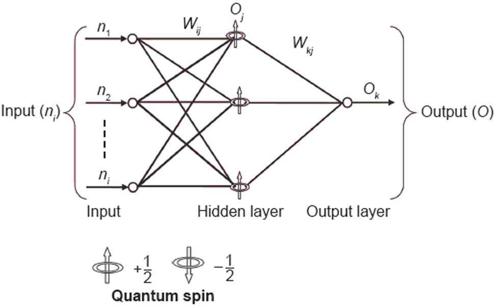
Architecture of quantum neural network.
Figure 6 depicts the QNN’s input, output, and hidden units. One occlusion layer is employed in this case. Each hidden-layer node represents three states, where r is the quantum level. For simplicity, we assume that n i means the input to the input layer, O j represents the output of the hidden layer, and O k represents the output of the output layer, representing the learning rate, which is a small random value.
As an illustration, n i represents the input layer, while O j and O k describe the hidden and output layers’ output, respectively. W ij represents a weight on the input layer, while W kj represents a weight on the hidden layer, and Figure 7 displays these relationships.
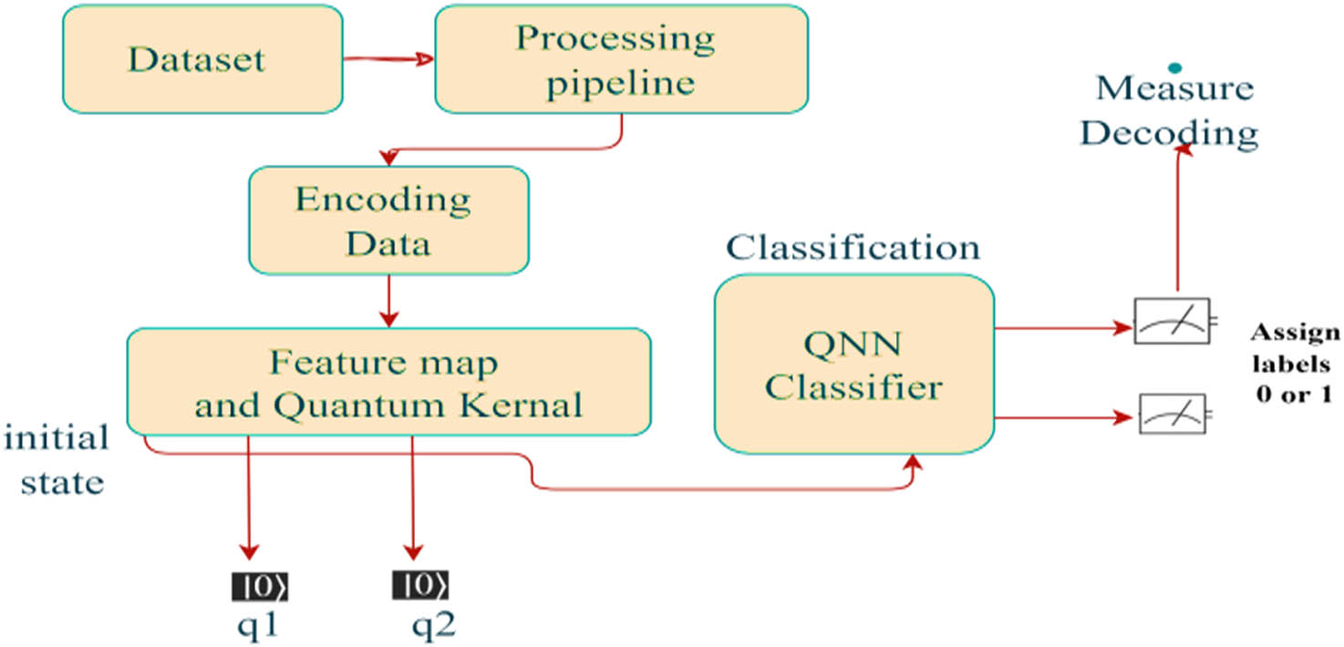
QNN classifier outline.
3.7.4 Quantum support vector machine (QSVM)
The SVM technique has a quantum counterpart in the QSVM approach. The Pegasos method, a fundamentally predicted subgradient solver for SVM, is used to train the classifier in the QSVM method. When applied to the SVM method, the quantum kernel technique accelerates the learning process, as seen in the QSVM algorithm. For processing on a quantum computer, the quantum kernel method uses quantum map features to convert standard data to quantum states. After training the QSVM classifier on a data set, its efficacy may be evaluated on a separate test data set. The classical-quantum (CQ) approach encodes classical data so that a quantum computer can handle it, enabling the mapping of conventional vectors of features to quantum spaces. The CQ method converts classical information into quantum states using a 5-qubit feature map. Figure 8 depicts the QSVM algorithm’s structure; the dataset is split between the training and testing datasets (in 80:20 proportion) after being preprocessed with RFE and min–max normalization. Computing the inner outcome of the quantum map features is how the quantum kernel transforms the quantum state of the collected information points into a space of higher dimension. To develop a QSVM for classification, a ZFeatureMap and a quantum kernel with a state vector simulator backend are used. The random seed of the algorithm is set to 12345. The CQ technique can be used to train the QSVM algorithm by encoding classical data to be processed by a quantum computer. The CQ technique employs a 5-qubit feature map to map classical feature vectors to quantum spaces. The quantum kernel changes the data points of the quantum state into a space with more dimensions by determining the inner outcome of the quantum map’s features. The model’s accuracy is determined by applying the QSVM classifier trained on the data to the test data and then analyzing the results. The QSVM algorithm is presented in Algorithm 4.
| Algorithm 4: The QSVM steps |
|---|
| Input: Training data |
| Output: A class label for feature vector |
| Begin |
| Step 1: Prepare the input, hidden layer(s), and output layers by setting their initial weights and biases. |
| Step 2: The epochs number and the learning rate may be adjusted. |
| Step3: Dividing a test dataset and a training dataset with an 80:20 split |
| Step 4: Preprocessing the dataset with RFE and min–max normalization. |
| Step 5: Applying a 5-qubit feature map to translate conventional feature vectors into quantum spaces. |
| Step 6: We take the inner result of the quantum map features to project the state of quantum data points into a higher dimensional space. |
| Step 7: The training data were used to fine-tune the QSVM classifier. |
| Step 8: Use the test data to determine how well the model performs. |
| Step 9: Decode the quantum information into its equivalent binary measurement (a standard value of 0 or 1) for each classical input. |
| End |
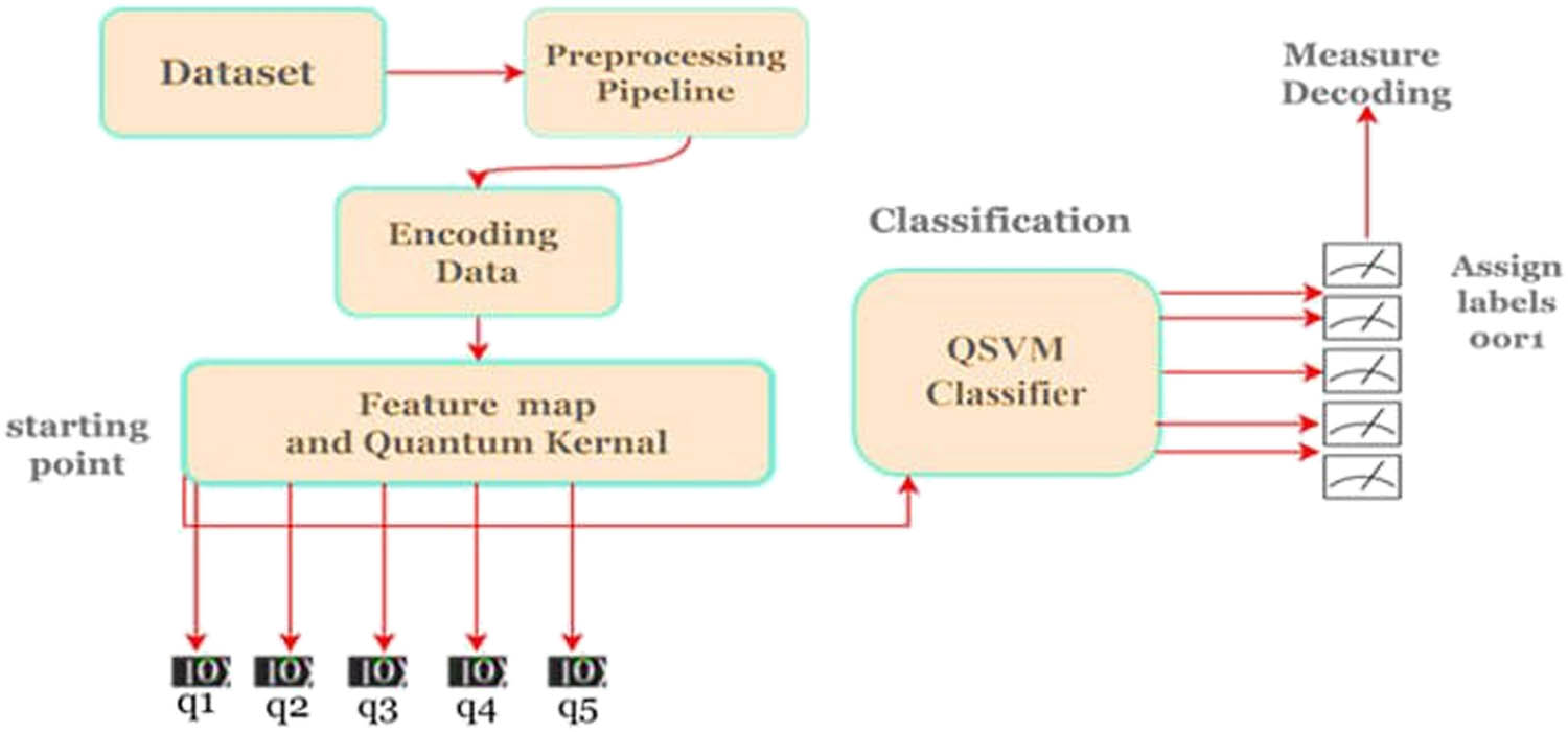
Outline of the QSVM.
The QSVM quantum kernel uses a quantum map of features to convert conventional vectors of features to quantum spaces. The traditional feature vector (x) is transformed into a quantum state
3.8 Proposed bagging QSVM method for HD diagnosis
HD classification is a crucial task in medical research, and ML methods have been extensively employed to improve classification models. Ensemble learning approaches, such as bagging, can be used to enhance the performance of HD model classification. To aggregate the classifications of many models trained on various parts of the same dataset, a technique called “bagging” is used. A new model relies on a bagging ensemble process built on top of the QSVM to efficiently classify HDs. The method utilizes a random method of splitting the dataset into smaller pieces. If the classification algorithm is not performing well in identifying the HD risk, using an ensemble strategy like boosting or bagging can help. Combining the best features of bagging and the QSVM algorithm, bagging-QSVM is an ensemble learning method that can make models work better. For this method, 100 separate QSVM models are trained on different parts of the dataset. The final output of the ensemble model is then generated by averaging the predictions of these models. After training the models, the ensemble model provides the final result by averaging the forecasts and assigning the majority vote to the class with the most votes. In each bootstrap sample utilized in the bagging model, some occurrences from the original dataset are duplicated or disregarded. Each bootstrap sample in a bagging model replicates the original dataset or skips part of the occurrences. This approach generates many subsamples of a dataset for use in model training. The bagging ensemble approach averages the predictions of several models, which is very useful when working with high-variance models because it helps reduce the model’s variance. When used in statistical learning or model fitting, the bagging ensemble method is an example of ensemble learning that integrates many models to enhance prediction performance. The bagging-QSVM algorithm is presented in Algorithm 5.
| Algorithm 5: Bagging-QSVM |
|---|
| Input: Training data |
| Output: A class label for feature vector |
| Begin |
| Step 1: Datasets are often divided into test and training sets. |
| Step2: For each bootstrap sample: |
| a. The training data should be sampled at random. |
| b. Training a QSVM algorithm on the specified subset. |
| c. Save the model after training. |
| Step 3: For each instance in the testing set: |
| a. Using all of the saved QSVM models to make predictions. |
| b. Considering a weighted majority vote, combine the forecasts. |
| Step 4: The Bagging-QSVM model is tested, and its results are analyzed. |
| Step 5: Returning the final output of the Bagging-QSVM model. |
| End |
Figure 9 presents a schematic description of the bagging-QSVM model:
The first step in converting conventional data into a quantum state is to define the quantum feature map.
In step two, the quantum feature map is used as an input parameter in constructing a new instance of the QSVM class.
Third, the QSVM instance is used as the basis estimator to create a new instance of the bagging classification class.
Fourth, the fit technique is used to adjust the bagging classification instance to the input data.
The classification approach is employed to make predictions on newly collected information.
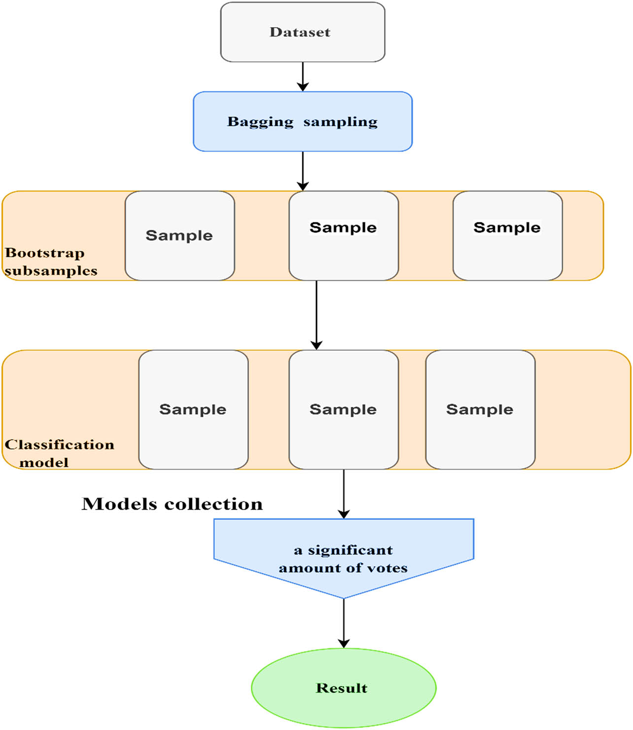
Bagging-QSVM model.
The bagging method keeps the QSVM algorithm from overfitting the data. The bagging approach produces several subsets of the original dataset by randomly picking data with replacement. A QSVM model is trained independently on each subgroup, and then, the models’ combined predictions are utilized to create a final classification.
4 Results and discussion
4.1 SVM results
When the models were trained on the comprehensive HD dataset, the achieved outcomes were are follows: accuracy of 73.1%, precision of 68% to abnormal and 79% to class normal, recall of 77% to class abnormal and 70% to class normal, F1 score of 72% to class abnormal and 74% to class normal, sensitivity of 80%, macro average of 73%, and average weight of 74%. All the results are summarized in Table 3.
Results obtained to evaluate the performance of the SVM model
| Model | Precision | Recall | F1 score | Iteration | Accuracy | |
|---|---|---|---|---|---|---|
| SVM | Abnormal | 0.68 | 0.77 | 0.72 | 107 | 0.73 |
| Normal | 0.79 | 0.70 | 0.74 | 131 | ||
| Macro/weighted average | 0.74 | 0.73 | 0.73 | 283 | ||
The classifier achieved a success rate of 73% in accurately categorizing the cases, as evidenced by its overall accuracy of 0.73. Nonetheless, accuracy alone may not provide a comprehensive understanding of the classifier’s performance. In terms of predicting the absence of HD, the classifier displayed a precision of 0.68 and exhibited a precision of 0.79 in predicting the presence of HD. Precision, which refers to the percentage of correctly anticipated occurrences for a given class, was appropriately exemplified. A high level of accuracy is indicated by a low occurrence of false positives. Specifically, the recall for identifying the presence of HD was 0.70, while the recall for determining its absence was 0.77. Recall is also referred to as sensitivity or true positive rate and measures the percentage of correctly predicted occurrences of actual positivity. A strong recall is indicated by a low rate of false negatives. On the one hand, in the case of forecasting the absence of cardiac disease, the F1 score, which is the harmonic mean of accuracy and recall, was reported to be 0.72. On the other hand, for predicting the presence of cardiac disease, the F1 score was reported to be 0.74. The F1 score provides a balanced metric that combines precision and recall. This metric is particularly useful in situations where the dataset is unbalanced. From the analysis of the performance metrics, we can infer that the classifier categorizes cases of HD. This is evident from the high accuracy, recall, and F1 score for both the absence and presence of cardiac disease, indicating a good balance between true positives and negatives. However, these metrics have different applications and are inversely related to each other. By examining these indicators, the effectiveness of the SVM model can be assessed, and areas that may require improvement can be identified.
The evaluation of the SVM classification algorithm for disease prediction pertaining to the heart involves the examination of a confusion matrix and the receiver operating characteristic (ROC) graph. The actual and predicted values are represented in Figure 10. The parity between the number of actual predictions from the normal and abnormal classes demonstrates the accuracy of the system. The ROC for the SVM is presented in Figure 11. This evaluation reveals the capability of the SVM in diagnosing patients with and without HD based on the classification analysis.
Confusion matrix the SVM model.
ROC curve of the SVM model.
The precision of the model for the normal class surpasses that of the abnormal class, suggesting that the likelihood of correct classification is greater when predicting a normal class than when predicting an abnormal class. Meanwhile, the recall of the model for the abnormal class outperforms that for the normal class, indicating that the model exhibits superior identification capabilities for abnormal cases compared with normal cases. Moreover, the F1 score of the model for the abnormal class exceeds that of the normal class, signifying that the model’s predictive capabilities are more accurate for the abnormal class than for the normal class. In terms of iteration, the model underwent more iterations for the normal class than for the abnormal class. This particular observation implies that the model received more training in the normal class, possibly contributing to the higher precision observed for the normal class than that for the abnormal class. The model’s accuracy is 0.73, indicating that it has accurately predicted 73% of the data. The SVM model demonstrated a satisfactory accuracy level of 0.73. However, when considering the precision, the recall, and the F1 score, the model’s performance varied between the abnormal and normal classes. The analysis of the results suggests that the model is more adept at identifying abnormal cases than normal cases, indicating a bias toward the normal class during training. Consequently, adjustments to the hyperparameters and fine-tuning of the model may be necessary to enhance the model’s performance.
4.2 ANN results
The following findings were obtained after training the models on the comprehensive HD dataset: accuracy of 83.61%, precision of 82% to abnormal and 0.85% to normal, recall of 81% to abnormal and 85% to normal, F1 score of 82% to abnormal and 85% to normal, and sensitivity of 80% in the ANN model. All the results are summarized in Table 4.
Important performance metrics used to evaluate the performance of the ANN model
| Model | Precision | Recall | F1 score | Iteration | Accuracy | |
|---|---|---|---|---|---|---|
| ANN | Normal | 0.82 | 0.81 | 0.82 | 107 | 0.84 |
| Abnormal | 0.85 | 0.85 | 0.85 | 131 | ||
| Macro/weighted avg | 0.83 | 0.83 | 0.83 | 283 | ||
The ANN classifier attained an accuracy of 0.84, indicating that it accurately classified 84% of the instances in the dataset. For abnormal cases, the precision is 0.82, denoting that 82% of the instances was predicted as not having HD were true negatives. For normal cases, the precision was 0.85, indicating that 85% of the instances predicted as having HD were true positives. In the case of abnormalities, the recall stood at 0.81, meaning that 81% of the instances without HD were correctly identified. For normal cases, the recall was 0.85, indicating that 85% of the instances with HD were correctly identified. The F1 score, a harmonic mean of precision and recall, was presumably calculated for both classes. The analysis of the performance metrics suggests that the ANN classifier exhibits commendable performance in the field of HD classification research, characterized by high precision, recall, and accuracy for both classes. The classifier’s balanced performance is further evidenced by its consistent macro average precision, recall, and F1 score. The confusion matrix can offer additional insights into the classifier’s performance by illustrating the number of true positives, true negatives, false positives, and false negatives for each class. The problem consists of abnormal and normal cases, and the model generated predictions for 238 cases.
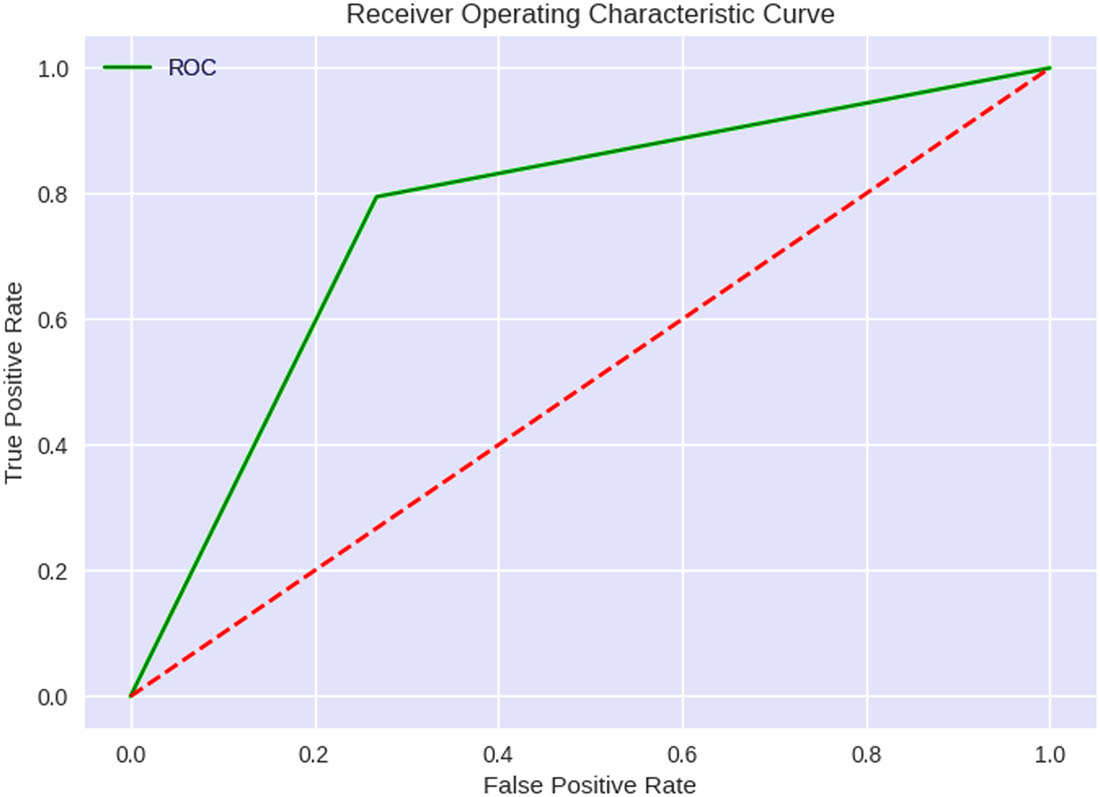
The performance of the ANN classification algorithm shown in Figure 12 was assessed using a confusion matrix and an ROC graph. In terms of performance metrics analysis, several insights can be drawn. First, the confusion matrix displays the combination of the actual and predicted values. This matrix reveals that the number of actual predictions was equal for the positive and negative classes, indicating the accuracy of the system. Second, the ROC curve is a graphical depiction of the performance of a binary classifier system as its recognition threshold is varied. Figure 13 presents the ROC curve for the ANN classifier, demonstrating the classifier’s high sensitivity and specificity in diagnosing patients with and without HD on the basis of the classification evaluation.
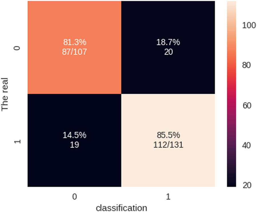
Confusion matrix of the ANN model.
ROC curve of the ANN model.
The precision score for the normal category was 0.82, while the precision score for the abnormal category was 0.85. These scores indicate that the model’s false positive predictions decreased, thus showcasing its proficiency in predicting positive cases. Furthermore, the recall score for the normal category was 0.81, and that for the abnormal category was 0.85. These scores suggest that the model’s false negative predictions were minimized, demonstrating its capability to identify positive cases. In addition, the F1 score for the normal category was 0.82, and that for the abnormal category was 0.85. These scores imply that the model’s false positive and false negative predictions decreased, thereby highlighting its aptitude for predicting and identifying positive cases. Precision, recall, and F1-score are significant metrics employed to evaluate the performance of a classification model. The iteration number pertains to the frequency with which a model is trained on the dataset. Depending on the nature of the problem and the available data, a certain measure or collection of metrics may be more suitable.
4.3 QNN results
The outcomes were as follows: accuracy of 77%, precision of 76% to class 0 and 77% to class 1, recall of 73% to class 0 and 79% to class 1, F1 score of 75% to class 0 and 78% to class 1, macro average of 0.77%, and average weight of 77% in the QSVM model. All the results are summarized in Table 5.
Results obtained to evaluate the performance of the QNN model
| Model | Precision | Recall | F1 score | Iteration | Accuracy | |
|---|---|---|---|---|---|---|
| QNN | Normal | 0.76 | 0.73 | 0.76 | 107 | 0.77 |
| Abnormal | 0.77 | 0.77 | 0.78 | 131 | ||
| Macro/weighted avg | 0.77 | 0.76 | 0.76 | 283 | ||
For predicting cardiac issues, the QNN classifier achieved a total accuracy rating of 0.77. This result proves that the classifier accurately classified HD patients. However, to fully grasp the classifier’s capabilities, the accuracy and recall for both the negative and positive categories must be examined. The respective precision and recall were 0.76 and 0.73 for the negative class, which represents those who do not have HD. Based on these measures, the classifier accurately identified healthy individuals. The respective accuracy and recall were 0.77 and 0.79 for the positive class, which represents those with HD. Based on these measurements, the classifier is also reasonably reliable in identifying people with HD. For the negative class, the F1 score was 0.75, and for the positive class, the F1 score was 0.78. F1 is a value that combines precision and recall. The results demonstrate that the ratio of accuracy to recall is satisfactory for both groups. The iteration value for the abnormal was determined to be 107. These metrics were derived by evaluating the confusion matrix and ROC graph of the QNN classifier in predicting HD. Thus, the QNN classifier achieved an overall performance of 0.77 in the prediction of HD, accompanied by reasonably reliable precision and recall for both the positive and negative classes. The F1 score level for both classes was commendable, thereby signifying a favorable balance between precision and recall. These metrics were obtained by assessing the confusion matrix and ROC graph of the QNN classifier for HD prediction, as illustrated in Figures 14 and 15.
Confusion matrix of the QNN model.
ROC curve of the QNN model.
Cross-validation constitutes a methodology employed for assessing the efficacy of a model by subjecting it to the examination of a portion of the data that were not employed during the training process. In the context of a QNN, the outcomes of cross-validation can be used to determine the optimal collection of parameter values. This implies that the parameters of the network can be modified to enhance its performance based on the outcomes of cross-validation, as depicted in Figure 16.
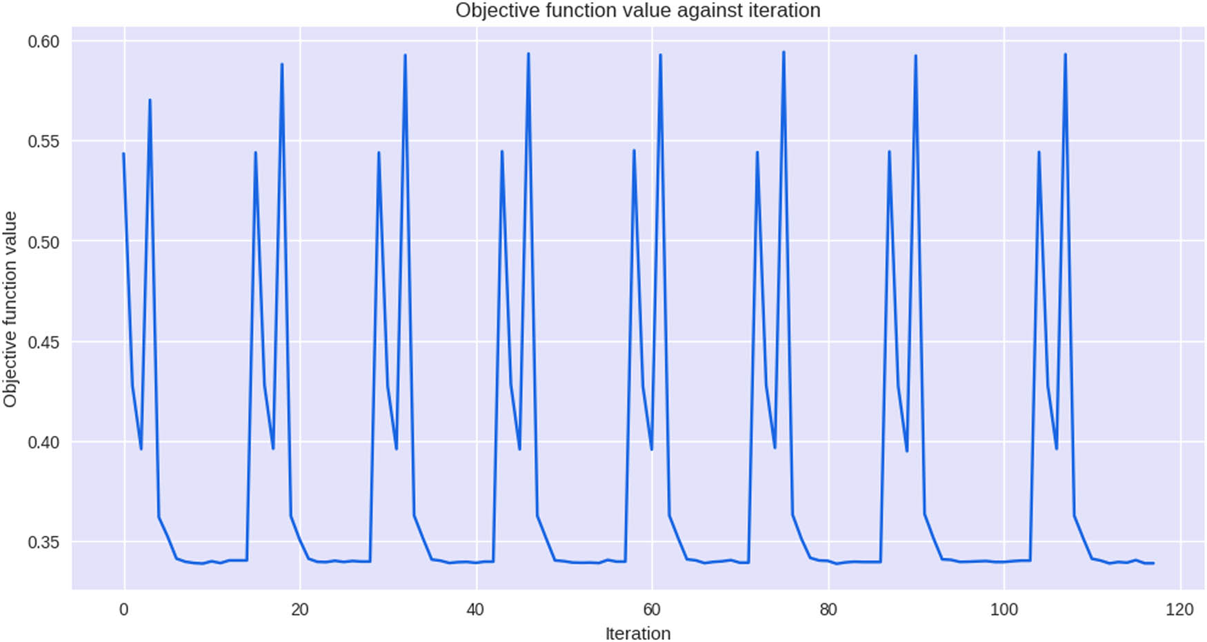
Cross-validation QNN model.
The analysis of these metrics indicates that the model exhibits a reduced number of false positive and false negative predictions for the normal category compared with the abnormal category. The F1 score serves as a means to strike a balance between precision and recall. Moreover, it signifies that the model manifests a lower occurrence of false positive and false negative predictions for the normal category than for the abnormal category. The accuracy of the model stands at 0.76, indicating that it accurately predicts the class of 76% of the data points. Precision, recall, F1 score, and accuracy are pivotal metrics employed to assess the performance of a classification model. These metrics offer valuable insights into the accuracy and quantity of the model’s positive predictions and the equilibrium between precision and recall. The selection of appropriate metric(s) is contingent on the problem domain and the dataset at hand.
4.4 Quantum support vector classifier results
The following results were obtained: accuracy of 85%, precision of 79% to class 0 and 91% to normal, recall of 90% to class 0 and 81% to class 1, F1 score of 84% to class 0 and 85% to class 1, macro average of 0.85, and average weight of 86% in the QSVM model. All the results are summarized in Table 6.
Results achieved to evaluate the performance of the QSVM model
| Model | Precision | Recall | F1 score | Iteration | Accuracy | |
|---|---|---|---|---|---|---|
| QSVM | Normal | 0.79 | 0.90 | 0.84 | 107 | 0.85 |
| Abnormal | 0.91 | 0.81 | 0.85 | 131 | ||
| Macro/weighted avg | 0.85 | 0.85 | 0.85 | 283 | ||
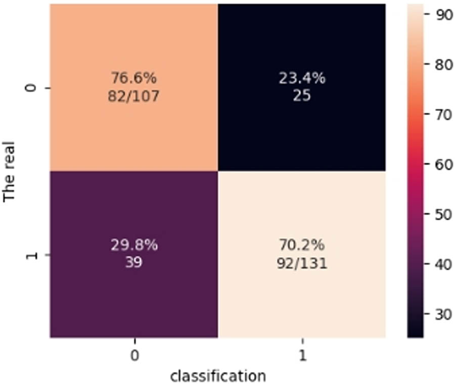
The measure known as recall, sensitivity, or true positive rate provides a quantitative assessment of the proportion of true positive predictions among all positive cases in the dataset. In an abnormal setting, the model correctly classified 90% of people as having no cardiac illness (recall = 0.90). The recall for normality was 0.81, indicating that the algorithm correctly identified 81% of people with HD. These recall values demonstrate the classifier’s ability to catch negative and positive examples accurately. The F1 score must be considered for a thorough investigation. The F1 score is the harmonic average of accuracy and recall and is a balanced statistic for assessing classifier performance. With an F1 score of 0.84, anomalies were classified with a good mix of accuracy and recall. Table 5 shows the accuracy and recall of the QSVM method, which lets us test how well it works in real life and find any problems. The total accuracy of the QSVM classifier on the dataset was 84%. The classifier achieved a precision of 0.79 for abnormality (no HD) and 0.91 for normalcy (HD). The recall for abnormal cases was 0.90, and that for normal cases was 0.81. Specifically, the F1 score for class 0 was 0.84, showing an excellent equilibrium between accuracy and recall. A more thorough investigation of a classifier’s efficacy may be conducted if its performance is measured across various parameters. Precision is the proportion of genuine positive predictions relative to all positive predictions made by the model, whereas accuracy describes how well the classifier can predict class labels. In contrast, recall quantifies the proportion of correct positive predictions relative to the total number of positive cases in a dataset. Finally, the F1 score is a balanced indication of classifier performance because it takes the harmonic mean of accuracy and recall.
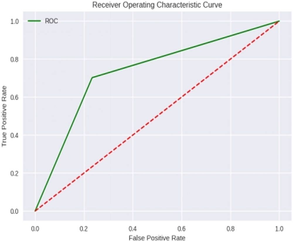
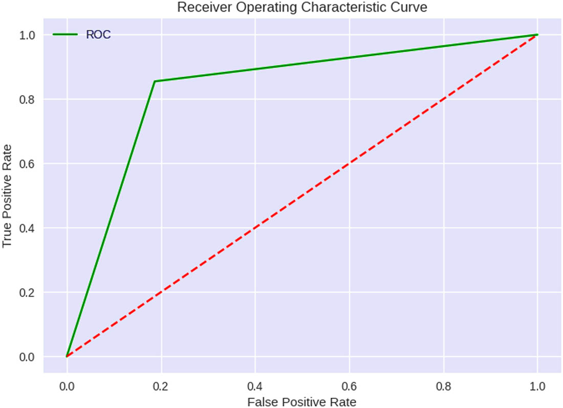
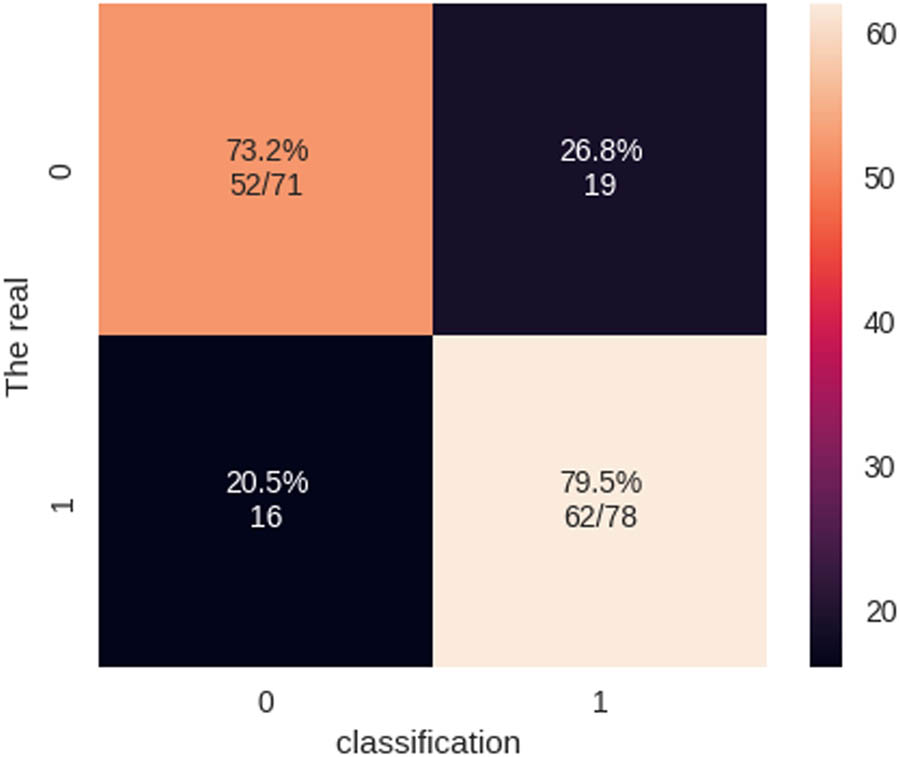
Using a quantum kernel, the QSVM method accelerates the SVM’s learning process, making it a QML algorithm. The Qiskit ML library includes a score function for determining the QSVM model’s precision. Both accuracy and recall must be considered while analyzing the QSVM model’s results. Comparatively, recall measures the percentage of correct responses among all recorded positives, while precision measures the rate of correct answers among all projected positives. The F1 score is a harmonic average of accuracy and recall and offers a balanced evaluation of the algorithm’s performance. The model performed well in normal and atypical situations, as indicated by a comparable F1 score. With incredible accuracy and F1 scores in both normal and abnormal cases, the QSVM model seems a viable strategy for predicting HD. However, the model’s accuracy might shift depending on the characteristics utilized for categorization and the data set. Common and valid approaches can be used to check how well binary classification methods, like QSVM, work for predicting HD. These approaches include confusion matrices and ROC curves, which show how well other models work. These methods can potentially enhance the HD prediction model’s accuracy and generalizability, which in turn will aid in halting the disease progression. ROC curves and confusion matrices test how well the QSVM algorithm works for classifying HD cases. These resources help determine whether a binary classification method performs as expected. The results of the confusion matrix and ROC curves are presented in Figures 17 and 18.
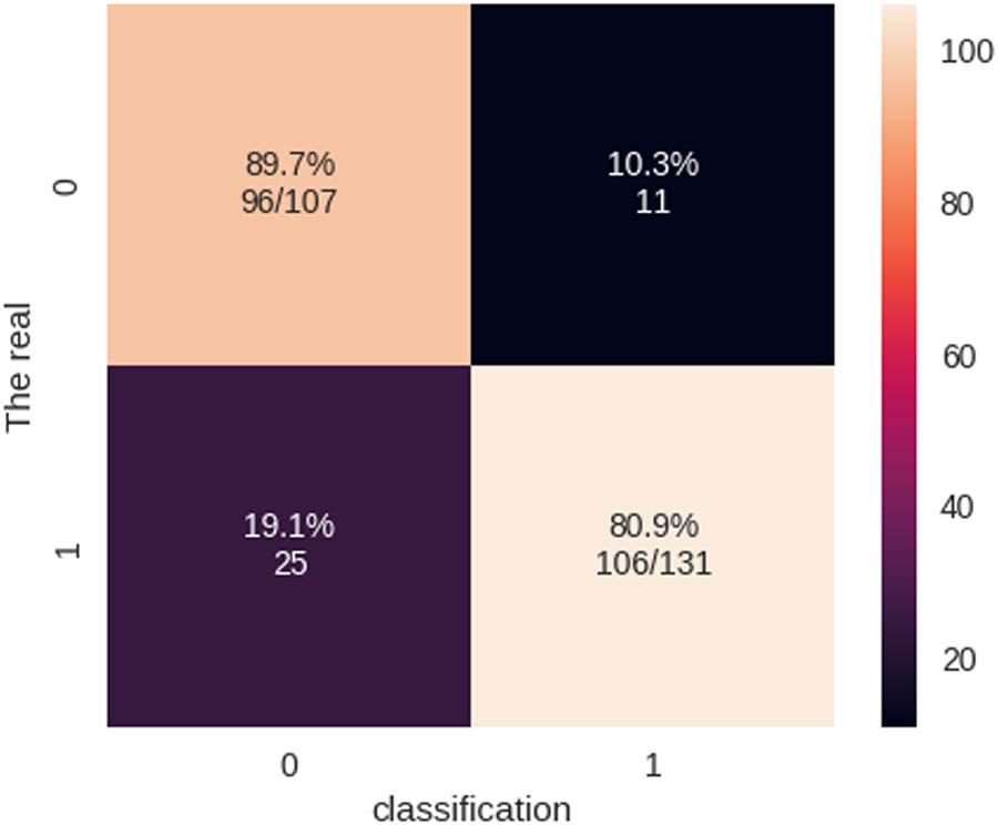
Confusion matrix of the QSVM model.
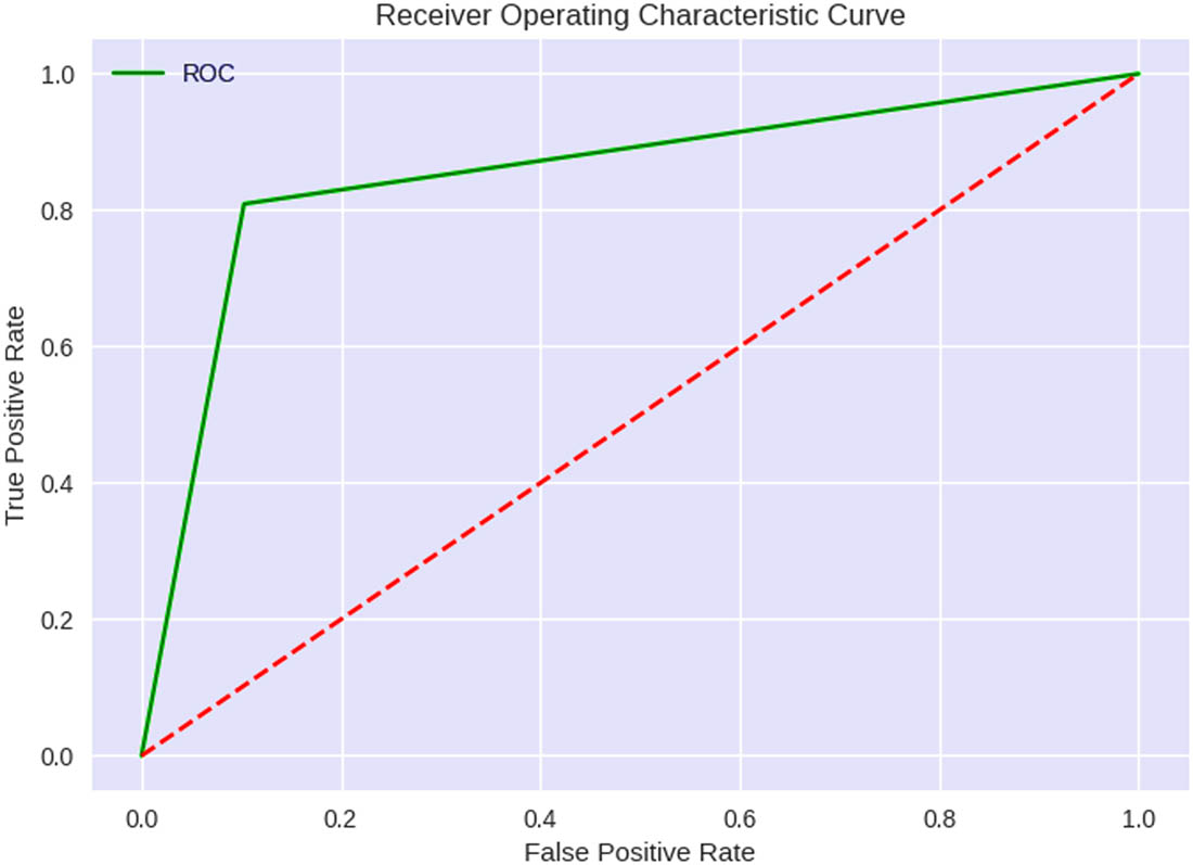
ROC curve of the QSVM model.
4.5 Experimental results of the proposed bagging model for HD diagnosis
The accuracy, precision, recall, F1 score, and average weight using bagging-QSVM were all determined to be optimal when the proposed method was implemented in the dataset and tested. Table 7 summarizes the results.
Results for evaluating the performance of the Bagging_QSVM model
| Model | Precision | Recall | F1 score | Iteration | Accuracy | |
|---|---|---|---|---|---|---|
| Bagging-QSVM | Normal | 1.00 | 1.00 | 1.00 | 107 | 1.00 |
| Abnormal | 1.00 | 1.00 | 1.00 | 131 | ||
| Macro/weighted avg | 1.00 | 1.00 | 1.00 | 283 | ||
The proposed approach achieved an accuracy of 100% when applied to the dataset, indicating that all data points were correctly classified. The precision for both the abnormal and normal classes was 100%, indicating that all predicted positive instances for both classes were positive. The recall for both abnormal and normal classes was 100%, indicating that the actual positive instances for both classes were correctly identified. The F1 score for both abnormal and normal classes was 100%, which is a harmonic mean of precision and recall, indicating a perfect balance between the two metrics. The macro average for precision, recall, and F1 score was 100%, indicating that the performance across both classes was excellent. The average weighted precision, recall, and F1 score in bagging-QSVM were also 100%, indicating a high level of performance across all classes.
The provided data appear to represent the evaluation measures of a model that has undergone training using the bagging technique along with QSVM. This specific model achieved a precision, recall, and F1 score of 1.00 for both the regular and abnormal categories. The accuracy of the model was also 1.00, indicating that the model did not made any incorrect predictions. For the regular and abnormal categories, the number of iterations was 107 and 131, respectively. In addition, the macro and weighted average for this model was 1.00. Bagging, a meta-algorithm within the domain of ML, was developed to improve the stability and accuracy of statistical classification and regression algorithms. This technique involves training multiple models on different subsets of the training data and then merging their predictions to generate a final prediction. While bagging enhances prediction accuracy, it does so at the expense of interpretability. Considering the aforementioned information, the model trained using bagging in conjunction with QSVM performs exceptionally well on the given task. The outcomes indicate that the bagging-QSVM model performed better than other ML methods, with precision, recall, and F1 scores of 1.00 as shown in Figures 19 and 20.
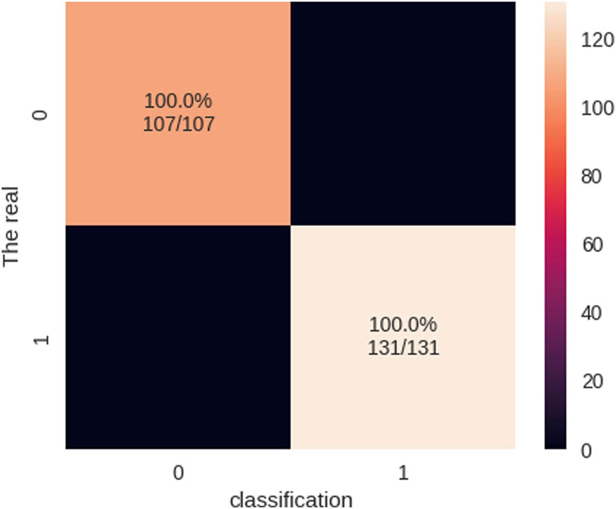
Confusion matrix of the bagging-QSVM model.
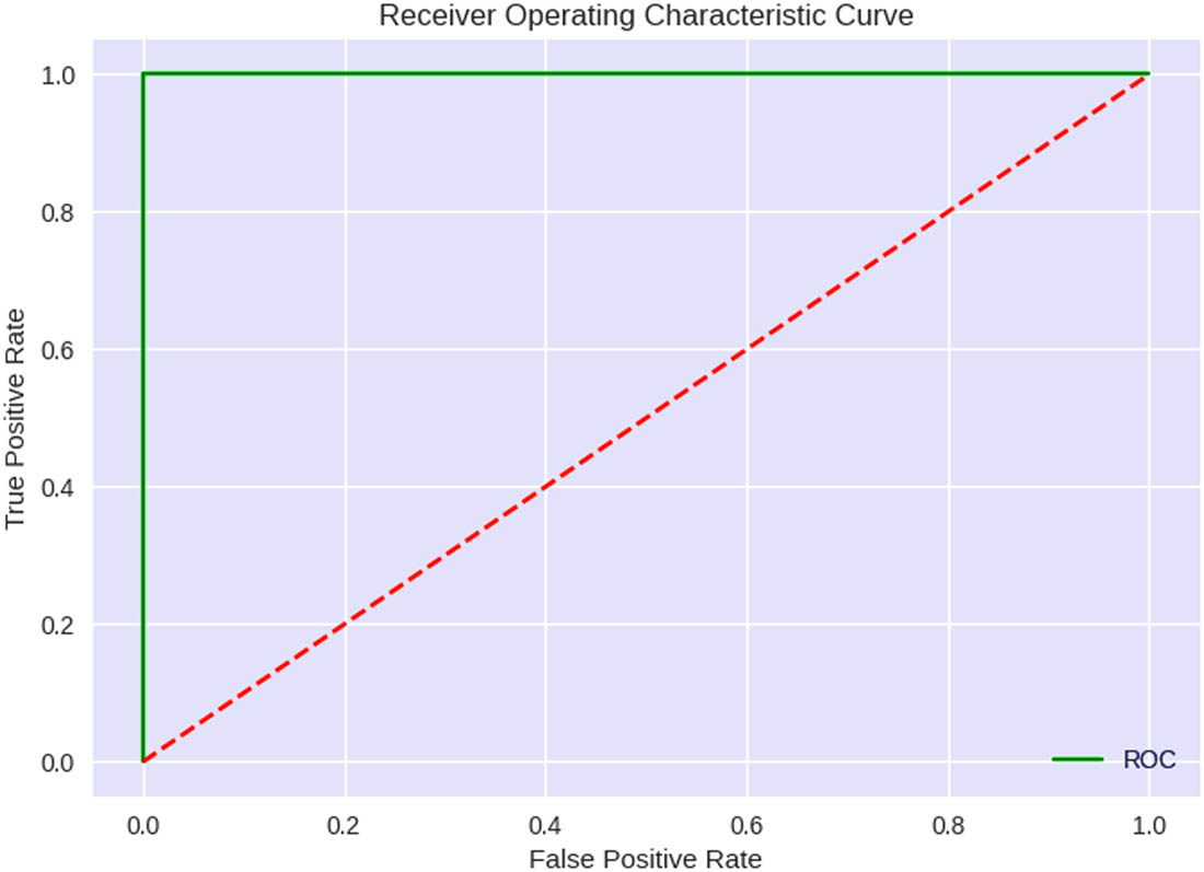
ROC curve of the bagging-QSVM model.
According to the findings of the experiment, the accuracy achieved by QSVM was recorded as 84.8%, whereas traditional SVM achieved an accuracy of 73.1%. Likewise, QNN demonstrated an accuracy of 76.5% in contrast to the 83.6% achieved by ANN. Therefore, QSVM and QNN exhibited the highest levels of performance among the quantum classifiers, with accuracies of 84.8 and 76.5%, respectively. On the one hand, this observation underscores the superior outcomes that quantum classifiers can generate compared with their classical classifier counterparts. On the other hand, the proposed model, known as bagging-QSVM, uses ensemble learning to show considerable improvements over previous quantum and classical classifiers. The bagging-QSVM surpasses all other methods, attaining an accuracy rate of 100%. Ensemble learning contributes to the optimization of quantum classifiers, as shown in Table 8.
Performance results of the classification models
| Classifier | Accuracy | Precision | Recall | F1 score |
|---|---|---|---|---|
| SVM | 73.1 | 69 | 75 | 73 |
| ANN | 83.6 | 84 | 83 | 84 |
| QNN | 76.5 | 77 | 76 | 77 |
| QSVM | 84.8 | 85 | 86 | 85 |
| Bagging-QSVM | 100 | 100 | 100 | 100 |
4.6 Comparison of the state of the arts
The results of the proposed method, which utilizes ensemble learning bagging-QSVM, were discussed and compared with the findings of related works. According to the data presented in Table 8, the proposed approach achieved a remarkable accuracy rate of 100%, surpassing the results of the study by Asif et al. [26], who achieved an accuracy of 98.15%. Furthermore, the precision, recall, F1 score, and Cohen’s kappa values for the proposed approach were 96.27, 98.72, 97.48, and 95.07%, respectively. Meanwhile, Kumari and Muthulakshmi [27] secured a position with an accuracy of 95.33%, precision of 99.18%, recall of 97.90%, and F1 score of 98.53% [9], with an accuracy of 90.16%, precision of 0.90%, recall of 0.90%, and F1 score of 0.90%. With their stacked classifier, [27] attained an accuracy of 86.49%, precision of 87.32%, recall of 86.02%, and F1 score of 86.01%. The ROC-area under the curve (AUC) for their model was 99. The ML ensemble method also performed admirably, with an F1 score of 88.70%, a precision and recall of 88.02%, and an accuracy of 88.70%. This model obtained a ROC-AUC of 93. In the study by [18], instance-based quantum DL and ML were used to obtain 98 and 83.6% accuracy rates, respectively. The bagging-QSVM model outperformed all other classifiers with 100% accuracy, precision, recall, and F1 score. Both binary and regression classification modeling objectives were used to evaluate the outcomes. The results show that better predictions may be obtained using bagging, which employs many models with high variation but low bias. Overall, the bagging-QSVM model demonstrated superior performance over other ensemble learning models when applied to HD prediction. Bagging, as a powerful ensemble learning method, effectively reduces variance and enhances model accuracy. In addition, QSVM, a quantum classifier with proven superiority over other quantum classifiers, can be effectively incorporated into the bagging model to achieve high-performance outcomes. Table 9 compares the results of the proposed approach with those of related works for HD prediction and shows that the proposed method achieved the highest accuracy and performance measures. The bagging-QSVM model used in the proposed method outperforms other classifiers and can be used to achieve high performance.
Comparison the proposed method’s outcomes with those of state-of-the-art methods
| The study/year | Accuracy (%) | Precision (%) | Recall (%) | F1 score (%) |
|---|---|---|---|---|
| Asif et al. (2023) [26] | 98.15 | 96.27 | 98.72 | 97.48 |
| Kumari and Muthulakshmi (2023) [27] | 95.33 | 99.18 | 97.90 | 98.53 |
| Abdulsalam et al. (2023) [9] | 90.16 | 90 | 90 | 90 |
| Alqahtani et al. (2022) [28] | 86.49 | 87.32 | 86.02 | 86.01 |
| Our study | 100 | 100 | 100 | 100 |
AI-based approaches have many uses, including detecting several diseases [29,30]. The proposed approach is to improve the accuracy and efficiency of HD classification by using cloud computing and quantum computing. While the cloud computing based on the framework that uses QML to classify heart diseases has great promise, it does have some significant limitations. First, there are not a lot of practical, scalable quantum processors available, and the science behind quantum computing is still in its early stages. This is a problem when trying to use large-scale QML algorithms to classify all forms of cardiac disease. Second, there may be compatibility problems with the current conventional infrastructure when integrating quantum techniques into cloud platforms, which might make deployment and interoperability more complicated. Last but not least, protecting private medical information in the cloud requires a comprehensive solution to the security issues surrounding quantum computing, including the possibility that quantum algorithms are susceptible to specific kinds of assaults. To overcome these constraints and properly utilize this unique method of heart disease categorization, there has to be continuous progress in quantum computing, improvements in integration strategies, and stronger security measures.
5 Conclusion
Early identification is crucial in slowing the progression of HD, which a significant cause of death. Therefore, this research aimed to investigate the utility of quantum ML in CVD risk prediction by developing a quantum-based ensemble learning model. As part of this research, we developed the bagging-QSVM model, which involves bagging the dataset into smaller groups and modeling each subset separately with QSVM. These groups are then joined using a majority vote system to form an ensemble. The classification accuracy of the proposed ensemble model on the Cleveland dataset was 90.16%, which is considerably higher than the accuracies of QSVM (88.52%), QNN (86.84%), VQC (85.25%), and SVC (85.24%). A wide range of performance indicators and ROC curves highlighted the suggested model’s superior performance over competing ML models. This research shows that quantum classifiers perform better than classical classifiers. The results also show the potential of ensemble learning methods for improving the efficiency of quantum classifiers. The methodology developed in this study shows promise in detecting early risk for HD, which might prevent catastrophic repercussions, and predicting and diagnosing other cardiovascular conditions.
Acknowledgments
We would like to confirm that all the figures were originally created by us.
-
Funding information: The authors received no specific funding for this study.
-
Author contributions: Huda Ghazi Enad: Conceptualization, Methodology, Formal analysis, Investigation, Writing – original draft, Visualization, Writing – review & editing. Mazin Abed Mohammed: Conceptualization, Methodology, Writing – review & editing, Project administration, Supervision.
-
Conflict of interest: The authors declare no conflict of interest.
-
Data availability statement: The HD dataset sourced from Kaggle is as a comprehensive compilation of HD-related data. The dataset merges information from five distinct datasets into a unified dataset. This merger extends across 12 common features, making it the most extensive HD dataset available for research purposes [23]. The five constituent datasets utilized for this are the Cleveland, Hungarian, Switzerland, Long Beach VA, and Statlog (Heart) datasets [24].
References
[1] Enad HG, Mohammed MA. A review on artificial intelligence and quantum machine learning for heart disease diagnosis: Current techniques, challenges and issues, recent developments, and future directions. Fusion: Pract Appl (FPA). 2023;11(1):08–25.10.54216/FPA.110101Suche in Google Scholar
[2] Sarra RR, Dinar AM, Mohammed MA. Enhanced accuracy for heart disease prediction using artificial neural network. Indones. J Electr Eng Comput Sci. 2022;29:375–83.10.11591/ijeecs.v29.i1.pp375-383Suche in Google Scholar
[3] Rahman AU, Saeed M, Mohammed MA, Jaber MM, Garcia-Zapirain B. A novel fuzzy parameterized fuzzy hypersoft set and riesz summability approach based decision support system for diagnosis of heart diseases. Diagnostics. 2022;12(7):1546.10.3390/diagnostics12071546Suche in Google Scholar PubMed PubMed Central
[4] Sarra RR, Dinar AM, Mohammed MA, Ghani MKA, Albahar MA. A robust framework for data generative and heart disease prediction based on efficient deep learning models. Diagnostics. 2022;12(12):2899.10.3390/diagnostics12122899Suche in Google Scholar PubMed PubMed Central
[5] Mastoi QUA, Wah TY, Mohammed MA, Iqbal U, Kadry S, Majumdar A, et al. Novel DERMA fusion technique for ECG heartbeat classification. Life. 2022;12(6):842.10.3390/life12060842Suche in Google Scholar PubMed PubMed Central
[6] Sarra RR, Dinar AM, Mohammed MA, Abdulkareem KH. Enhanced heart disease prediction based on machine learning and χ2 statistical optimal feature selection model. Designs. 2022;6(5):87.10.3390/designs6050087Suche in Google Scholar
[7] Rahman AU, Saeed M, Mohammed MA, Krishnamoorthy S, Kadry S, Eid F. An integrated algorithmic MADM approach for heart diseases’ diagnosis based on neutrosophic hypersoft set with possibility degree-based setting. Life. 2022;12(5):729.10.3390/life12050729Suche in Google Scholar PubMed PubMed Central
[8] Maheshwari D, Ullah U, Marulanda PAO, Jurado AGO, Gonzalez ID, Merodio JMO, et al. Quantum machine learning applied to electronic healthcare records for ischemic heart disease classification. Hum-Cent Comput Inf Sci. 2023;13(6):1–17.Suche in Google Scholar
[9] Abdulsalam G, Meshoul S, Shaiba H. Explainable heart disease prediction using ensemble-quantum machine learning approach. Intell Autom Soft Comput. 2023;36:761–79. 10.32604/iasc.2023.032262.Suche in Google Scholar
[10] Munshi M, Gupta R, Jadav NK, Polkowski Z, Tanwar S, Alqahtani F, et al. Quantum machine learning‐based framework to detect heart failures in Healthcare 4.0. Software: Pract Experience. 2024;54(2):168–85.10.1002/spe.3264Suche in Google Scholar
[11] Maheshwari D, Garcia-Zapirain B, Sierra-Soso D. Machine learning applied to diabetes dataset using Quantum versus Classical computation. In 2020 IEEE international symposium on signal processing and information technology (ISSPIT). IEEE; 2020, December. p. 1–6.10.1109/ISSPIT51521.2020.9408944Suche in Google Scholar
[12] Gupta H, Varshney H, Sharma TK, Pachauri N, Verma OP. Comparative performance analysis of quantum machine learning with deep learning for diabetes prediction. Complex & Intell Syst. 2022;8(4):3073–87.10.1007/s40747-021-00398-7Suche in Google Scholar
[13] Zhang Y, Ni Q. Recent advances in quantum machine learning. Quantum Eng. 2020;2(1):e34.10.1002/que2.34Suche in Google Scholar
[14] Blance A, Spannowsky M. Quantum machine learning for particle physics using a variational quantum classifier. J High Energy Phys. 2021;2021(2):1–20.10.1007/JHEP02(2021)212Suche in Google Scholar
[15] Yildirim O, Baloglu UB, Talo M, Ganesan P, Tung JS, Kang G, et al. Deep neural network trained on surface ECG improves diagnostic accuracy of prior myocardial infarction over Q wave analysis. In 2021 Computing in Cardiology (CinC). 48, IEEE; 2021, September. p. 1–4.10.23919/CinC53138.2021.9662825Suche in Google Scholar
[16] Li X, Li C, Wei Y, Sun Y, Wei J, Li X, et al. Bat: Beat-aligned transformer for electrocardiogram classification. In 2021 IEEE International Conference on Data Mining (ICDM). IEEE; 2021, December. p. 320–9.10.1109/ICDM51629.2021.00043Suche in Google Scholar
[17] Elsedimy EI, AboHashish SMM, Algarni F. New cardiovascular disease prediction approach using support vector machine and quantum-behaved particle swarm optimization. Multimed Tools Appl. 2023;1–28. 10.1007/s11042-023-16194-z.Suche in Google Scholar
[18] Alsubai S, Alqahtani A, Binbusayyis A, Sha M, Gumaei A, Wang S. Heart failure detection using instance quantum circuit approach and traditional predictive analysis. Mathematics. Mar. 2023;11(6):1467. 10.3390/math11061467.Suche in Google Scholar
[19] Kavitha SS, Kaulgud N. Quantum K-means clustering method for detecting heart disease using quantum circuit approach. Soft Comput. 2022;27(18):13255–68. 10.1007/s00500-022-07200-x.Suche in Google Scholar PubMed PubMed Central
[20] Heidari H, Hellstern G. Early heart disease prediction using hybrid quantum classification. arXiv:2208.08882.Suche in Google Scholar
[21] Ozpolat Z, Karabatak M. Performance evaluation of quantum-based machine learning algorithms for cardiac arrhythmia classification. Diagnostics. Mar. 2023;13(6):1099. 10.3390/diagnostics13061099.Suche in Google Scholar PubMed PubMed Central
[22] Ullah U, Jurado AGO, Gonzalez ID, Garcia-Zapirain B. A fully connected quantum convolutional neural network for classifying ischemic cardiopathy. IEEE Access. 2022;10:134592–605. 10.1109/ACCESS.2022.3232307 Suche in Google Scholar
[23] “Heart Disease Dataset (Comprehensive) | IEEE DataPort.” Accessed: Dec. 22, 2023. [Online]. https://ieee-dataport.org/open-access/heart-disease-dataset-comprehensive.Suche in Google Scholar
[24] “Heart Disease Dataset (Comprehensive) | Kaggle.” Accessed: Feb. 07, 2023. [Online]. https://www.kaggle.com/datasets/sid321axn/heart-statlog-cleveland-hungary-final.Suche in Google Scholar
[25] Narain R, Saxena S, Goyal AK. Cardiovascular risk prediction: A comparative study of Framingham and quantum neural network-based approach. Patient Prefer Adherence. Jul. 2016;10:1259–70. 10.2147/PPA.S108203.Suche in Google Scholar PubMed PubMed Central
[26] Asif D, Bibi M, Arif MS, Mukheimer A. Enhancing heart disease prediction through ensemble learning techniques with hyperparameter optimization. Algorithms. Jun. 2023;16(6):308. 10.3390/a16060308.Suche in Google Scholar
[27] Kumari S, Muthulakshmi P. The necessity of artificial intelligence for smart environment: Future perspective and research challenges. In 2023 International Conference on Computer Communication and Informatics, ICCCI 2023; 2023. 10.1109/ICCCI56745.2023.10128362.Suche in Google Scholar
[28] Alqahtani A, Alsubai S, Sha M, Vilcekova L, Javed T. Cardiovascular disease detection using ensemble learning. Comput Intell Neurosci. 2022;2022:5267498. 10.1155/2022/5267498.Suche in Google Scholar PubMed PubMed Central
[29] Rizvi SQA, Wang G, Khan A, Hasan MK, Ghazal TM, Khan AUR. Classifying Parkinson’s disease using resting state electroencephalogram signals and U EN-PDNet. IEEE Access. 2023;11:107703–24.10.1109/ACCESS.2023.3319248Suche in Google Scholar
[30] Albadr MAA, Ayob M, Tiun S, Al-Dhief FT, Hasan MK. Gray wolf optimization-extreme learning machine approach for diabetic retinopathy detection. Front Public Health. 2022;10:925901.10.3389/fpubh.2022.925901Suche in Google Scholar PubMed PubMed Central
© 2024 the author(s), published by De Gruyter
This work is licensed under the Creative Commons Attribution 4.0 International License.
Artikel in diesem Heft
- Research Articles
- A study on intelligent translation of English sentences by a semantic feature extractor
- Detecting surface defects of heritage buildings based on deep learning
- Combining bag of visual words-based features with CNN in image classification
- Online addiction analysis and identification of students by applying gd-LSTM algorithm to educational behaviour data
- Improving multilayer perceptron neural network using two enhanced moth-flame optimizers to forecast iron ore prices
- Sentiment analysis model for cryptocurrency tweets using different deep learning techniques
- Periodic analysis of scenic spot passenger flow based on combination neural network prediction model
- Analysis of short-term wind speed variation, trends and prediction: A case study of Tamil Nadu, India
- Cloud computing-based framework for heart disease classification using quantum machine learning approach
- Research on teaching quality evaluation of higher vocational architecture majors based on enterprise platform with spherical fuzzy MAGDM
- Detection of sickle cell disease using deep neural networks and explainable artificial intelligence
- Interval-valued T-spherical fuzzy extended power aggregation operators and their application in multi-criteria decision-making
- Characterization of neighborhood operators based on neighborhood relationships
- Real-time pose estimation and motion tracking for motion performance using deep learning models
- QoS prediction using EMD-BiLSTM for II-IoT-secure communication systems
- A novel framework for single-valued neutrosophic MADM and applications to English-blended teaching quality evaluation
- An intelligent error correction model for English grammar with hybrid attention mechanism and RNN algorithm
- Prediction mechanism of depression tendency among college students under computer intelligent systems
- Research on grammatical error correction algorithm in English translation via deep learning
- Microblog sentiment analysis method using BTCBMA model in Spark big data environment
- Application and research of English composition tangent model based on unsupervised semantic space
- 1D-CNN: Classification of normal delivery and cesarean section types using cardiotocography time-series signals
- Real-time segmentation of short videos under VR technology in dynamic scenes
- Application of emotion recognition technology in psychological counseling for college students
- Classical music recommendation algorithm on art market audience expansion under deep learning
- A robust segmentation method combined with classification algorithms for field-based diagnosis of maize plant phytosanitary state
- Integration effect of artificial intelligence and traditional animation creation technology
- Artificial intelligence-driven education evaluation and scoring: Comparative exploration of machine learning algorithms
- Intelligent multiple-attributes decision support for classroom teaching quality evaluation in dance aesthetic education based on the GRA and information entropy
- A study on the application of multidimensional feature fusion attention mechanism based on sight detection and emotion recognition in online teaching
- Blockchain-enabled intelligent toll management system
- A multi-weapon detection using ensembled learning
- Deep and hand-crafted features based on Weierstrass elliptic function for MRI brain tumor classification
- Design of geometric flower pattern for clothing based on deep learning and interactive genetic algorithm
- Mathematical media art protection and paper-cut animation design under blockchain technology
- Deep reinforcement learning enhances artistic creativity: The case study of program art students integrating computer deep learning
- Transition from machine intelligence to knowledge intelligence: A multi-agent simulation approach to technology transfer
- Research on the TF–IDF algorithm combined with semantics for automatic extraction of keywords from network news texts
- Enhanced Jaya optimization for improving multilayer perceptron neural network in urban air quality prediction
- Design of visual symbol-aided system based on wireless network sensor and embedded system
- Construction of a mental health risk model for college students with long and short-term memory networks and early warning indicators
- Personalized resource recommendation method of student online learning platform based on LSTM and collaborative filtering
- Employment management system for universities based on improved decision tree
- English grammar intelligent error correction technology based on the n-gram language model
- Speech recognition and intelligent translation under multimodal human–computer interaction system
- Enhancing data security using Laplacian of Gaussian and Chacha20 encryption algorithm
- Construction of GCNN-based intelligent recommendation model for answering teachers in online learning system
- Neural network big data fusion in remote sensing image processing technology
- Research on the construction and reform path of online and offline mixed English teaching model in the internet era
- Real-time semantic segmentation based on BiSeNetV2 for wild road
- Online English writing teaching method that enhances teacher–student interaction
- Construction of a painting image classification model based on AI stroke feature extraction
- Big data analysis technology in regional economic market planning and enterprise market value prediction
- Location strategy for logistics distribution centers utilizing improved whale optimization algorithm
- Research on agricultural environmental monitoring Internet of Things based on edge computing and deep learning
- The application of curriculum recommendation algorithm in the driving mechanism of industry–teaching integration in colleges and universities under the background of education reform
- Application of online teaching-based classroom behavior capture and analysis system in student management
- Evaluation of online teaching quality in colleges and universities based on digital monitoring technology
- Face detection method based on improved YOLO-v4 network and attention mechanism
- Study on the current situation and influencing factors of corn import trade in China – based on the trade gravity model
- Research on business English grammar detection system based on LSTM model
- Multi-source auxiliary information tourist attraction and route recommendation algorithm based on graph attention network
- Multi-attribute perceptual fuzzy information decision-making technology in investment risk assessment of green finance Projects
- Research on image compression technology based on improved SPIHT compression algorithm for power grid data
- Optimal design of linear and nonlinear PID controllers for speed control of an electric vehicle
- Traditional landscape painting and art image restoration methods based on structural information guidance
- Traceability and analysis method for measurement laboratory testing data based on intelligent Internet of Things and deep belief network
- A speech-based convolutional neural network for human body posture classification
- The role of the O2O blended teaching model in improving the teaching effectiveness of physical education classes
- Genetic algorithm-assisted fuzzy clustering framework to solve resource-constrained project problems
- Behavior recognition algorithm based on a dual-stream residual convolutional neural network
- Ensemble learning and deep learning-based defect detection in power generation plants
- Optimal design of neural network-based fuzzy predictive control model for recommending educational resources in the context of information technology
- An artificial intelligence-enabled consumables tracking system for medical laboratories
- Utilization of deep learning in ideological and political education
- Detection of abnormal tourist behavior in scenic spots based on optimized Gaussian model for background modeling
- RGB-to-hyperspectral conversion for accessible melanoma detection: A CNN-based approach
- Optimization of the road bump and pothole detection technology using convolutional neural network
- Comparative analysis of impact of classification algorithms on security and performance bug reports
- Cross-dataset micro-expression identification based on facial ROIs contribution quantification
- Demystifying multiple sclerosis diagnosis using interpretable and understandable artificial intelligence
- Unifying optimization forces: Harnessing the fine-structure constant in an electromagnetic-gravity optimization framework
- E-commerce big data processing based on an improved RBF model
- Analysis of youth sports physical health data based on cloud computing and gait awareness
- CCLCap-AE-AVSS: Cycle consistency loss based capsule autoencoders for audio–visual speech synthesis
- An efficient node selection algorithm in the context of IoT-based vehicular ad hoc network for emergency service
- Computer aided diagnoses for detecting the severity of Keratoconus
- Improved rapidly exploring random tree using salp swarm algorithm
- Network security framework for Internet of medical things applications: A survey
- Predicting DoS and DDoS attacks in network security scenarios using a hybrid deep learning model
- Enhancing 5G communication in business networks with an innovative secured narrowband IoT framework
- Quokka swarm optimization: A new nature-inspired metaheuristic optimization algorithm
- Digital forensics architecture for real-time automated evidence collection and centralization: Leveraging security lake and modern data architecture
- Image modeling algorithm for environment design based on augmented and virtual reality technologies
- Enhancing IoT device security: CNN-SVM hybrid approach for real-time detection of DoS and DDoS attacks
- High-resolution image processing and entity recognition algorithm based on artificial intelligence
- Review Articles
- Transformative insights: Image-based breast cancer detection and severity assessment through advanced AI techniques
- Network and cybersecurity applications of defense in adversarial attacks: A state-of-the-art using machine learning and deep learning methods
- Applications of integrating artificial intelligence and big data: A comprehensive analysis
- A systematic review of symbiotic organisms search algorithm for data clustering and predictive analysis
- Modelling Bitcoin networks in terms of anonymity and privacy in the metaverse application within Industry 5.0: Comprehensive taxonomy, unsolved issues and suggested solution
- Systematic literature review on intrusion detection systems: Research trends, algorithms, methods, datasets, and limitations