Ensemble learning and deep learning-based defect detection in power generation plants

Marcellin Atemkeng; Victor Osanyindoro; Rockefeller Rockefeller; Sisipho Hamlomo; Jecinta Mulongo; Theophilus Ansah-Narh; Franklin Tchakounté; Arnaud Nguembang Fadja

doi:10.1515/jisys-2023-0283

Article Open Access

Ensemble learning and deep learning-based defect detection in power generation plants

Marcellin Atemkeng , Victor Osanyindoro , Rockefeller Rockefeller , Sisipho Hamlomo , Jecinta Mulongo , Theophilus Ansah-Narh , Franklin Tchakounté and Arnaud Nguembang Fadja

Published/Copyright: November 6, 2024

Published by

Become an author with De Gruyter Brill

Submit Manuscript Author Information

From the journal Journal of Intelligent Systems Volume 33 Issue 1

Abstract

One of the key factors driving a country’s economic development and ensuring the sustainability of its industries is the constant availability of electricity. This is normally provided by the national grid. However, the power supply is not always stable in developing countries where new businesses, including the telecommunications industry, are constantly emerging. Therefore, they must rely on generators to ensure their full functionality. These generators rely on fuel to function, and consumption is usually high if not properly monitored. Monitoring is usually done by a (non-expert) human. This can sometimes be a tedious process, as some companies have reported excessively high consumption rates. For anomaly detection in power generating plants, the studies by Mulongo et al. and Atemkeng and Jimoh used the same dataset to train a multilayer perceptron (MLP) and generative adversarial networks (GANs), respectively, achieving an accuracy of 96.1% with MLP and 98.9% with GAN. Through comparative analysis and the use of ensemble learning techniques, we found that ensemble learning models outperform both MLP and GAN as proposed by Mulongo et al. and Atemkeng and Jimoh using the same dataset. Furthermore, we investigated the potential of autoencoders to outperform MLPs, GANs, and ensemble learning models. To this end, we have introduced a label-assisted autoencoder approach for detecting anomalies in power-generating plants. This model includes a labelling assistance module that adjusts the thresholds. Our results indicate that the label-assisted autoencoder outperforms the MLP. However, GANs and all ensemble learning models outperformed the label-assisted autoencoder. Nevertheless, the use of a label-assisted autoencoder offers a distinct advantage in categorizing anomalies based on their severity, a capability not present in ensemble learning models and GANs.

Keywords: electric grid; fuel consumption; autoencoder; anomaly detection; power generating plants; GANs; ensemble learning

1 Introduction

Information communication technology companies use about 3% of the world’s electrical energy, and the telecommunication industry is one of the fastest growing industrial sectors among agriculture, banking, infrastructure, and oil and gas [1]. The number of telecommunication industries and the quest for expansion and growth has led to an increase in base stations across targeted countries to boost their network coverage and enhance the effective flow of communication. With the increase in the number of base stations, the issue of base station management needs to be addressed. Grid energy has been known to be the main source of power in developing countries such as those in Africa, and it is expected that these base stations located across different rural and urban areas will be powered by grid energy. However, electricity is quite unstable in most parts of these developing countries, and this has forced base stations to look for a reliable alternative source of energy. These alternatives include photovoltaic (PV) panels, wind turbines, and diesel generators, but mostly generators due to a lack of space for the installation of PV or wind turbines [2]. The high cost of fuel and its transportation to supply stations located in rural areas has increased the operational cost of these companies. These generators are being refilled manually, thus creating room for irregular or unusual fuel consumption, which might be caused by several reasons, such as fuel theft, fuel leakages, or poor maintenance of equipment. A study conducted in a base station in Cameroon has shown that the design of the base station building, room cooling systems such as air conditioners, and careless handling of lights increase the rate of fuel consumption in the base station [3]. Espadafor et al. [4] also attested that generator performance could be affected by the age of the generator, the number of loads powered by the generator, and improper maintenance.

In Cameroon, TeleInfra LTD is one such company whose objective is to manage base stations in various parts of the country. The services include maintenance of base stations and refuelling of generators. Like any other businesses relying on grid energy, the unstable power supply has resulted in high operating costs as companies have to find alternative sources of power supply to sustain the continuous operations of the business. Alternative sources such as solar panels, hybrid energy, and generators have been implemented by TeleInfra to sustain business performance. Data on fuel consumed, such as working hours of the generator, the quantity of fuel refuelled, the rate of consumption, generator maintenance, and total fuel consumed, are collected from base stations [5].

Many strategies have been proposed to improve energy saving, such as building a well-ventilated base station and the use of air conditioners as a cooling system and heat pipes to remove hot air from the base station [6]. However, detecting such irregularities is challenging, especially when numerous base stations are functioning at once. Anomaly detection in power-generating plants is aimed at detecting such irregularities in the behaviour of the data provided. Although there are different algorithms for detecting anomalies, machine learning algorithms are the most used and popular for anomaly detection due to their ability for automation and their effectiveness in the context of deep learning, especially when involving large datasets. According to Goodfellow et al. [7], deep learning is a variant of applied statistics with an increasing emphasis on using computers to estimate complex functions statistically but a reduced emphasis on proving confidence intervals around these functions. Machine learning algorithms come in several variants. In supervised learning, models can make predictions on unlabelled data after they have been trained on labelled data, whereas, in unsupervised learning, models can only make predictions on unlabelled data by learning similar features and patterns embedded in the datasets. In reinforcement learning, a goal is given, and an agent undergoes training in an environment to find an optimal solution to accomplish the goal.

Anomalies can be an indicator of areas that require attention, and detecting them has been quite popular among the research community. In the past, the research community has conducted several anomaly detections ranging from comprehensive to certain application domains with different machine learning algorithms. Mulongo et al. [5] worked on a similar area; four different supervised learning algorithms were used in their work for detecting an anomaly in a power generation plant. The dataset used by Mulongo et al. [5] was also employed by Atemkeng and Jimoh [8] to investigate and detect anomalies using generative adversarial networks (GANs). GANs are a supervised learning algorithm that involves training a classifier to assign a probability score to a sample, indicating whether it is categorized as “normal” or “anomalous.” However, in real-life scenarios, abnormal behavioural patterns are very few compared to normal behaviour. For instance, Atemkeng and Jimoh [8] had to duplicate the data to balance between normal and anomalous data before training the GANs. These are key challenges in recognizing anomalies with a deep supervised learning algorithm such as GAN since they greatly rely on labelling and balance between normal and anomalous data patterns. Our study initially explored ensemble learning models for anomaly detection in power-generating plants, using the same dataset as in the studies by Mulongo et al. [5] and Atemkeng and Jimoh [8]. Six ensemble learning models were investigated: adaptive boosting (Adaboost), categorical boosting (CatBoost), eXtreme gradient boosting (XGBoost), light gradient boosting machine (LightGBM), gradient boosted decision trees (GBDT), and random forest (RF). When trained on the same dataset, we observed that these models outperformed those proposed in the studies by Mulongo et al. [5] and Atemkeng and Jimoh [8]. Note that the shallow models trained in the study by Mulongo et al. [5] did not require the balancing of normal and abnormal samples, a characteristic that we observed in the ensemble learning methods as well during training. However, balancing the data was necessary to train the GAN discussed [8]. This is because GANs, being very deep, can overfit quickly when the dataset is unbalanced. By using the same dataset, we explored an alternative deep learning approach for anomaly detection based on unsupervised learning. The proposed framework modifies and fine-tunes a deep autoencoder, thus eliminating the need for data balancing required by the GAN. In addition, we incorporated a module into the autoencoder that uses labelled data to determine the autoencoder threshold. Depending on the outcome, one of the following actions is taken:

Update the threshold of the autoencoder to increase overall model accuracy to an acceptable level.
Adjust the interval of variation for numerical hyperparameters, enabling exploration of the best hyperparameter values in the new search space.
Provide an overall performance score.

This article is organized as follows: Section 2 explains anomaly detection and investigates related works for anomaly detection in power grid plants. Section 3 discusses ensemble learning and autoencoders, which replicate the input data through a compressed representation. This section also discusses the different evaluation metrics used in this work, proposes the label-assisted autoencoder, and provides a detailed discussion. The dataset and feature engineering are also discussed. Section 4 discusses the results and limitations, and Section 5 concludes the work.

2 Anomaly detection and related works

Anomalies, also known as outliers, often refer to instances or data samples that are significantly distanced from the main body of an examined data [9]. These distanced values often indicate a deviation from its established normal pattern, which can sometimes be a measurement error or an indication of a data sample of a different population [10]. Outlier classification depends on the type and domain of the given data as well as the data analyst. Since many outliers are linked directly with abnormal behaviour, they are also referred to as deviants, anomalies, or abnormalities in the literature of statistics and data analysis [9]. According to Aggarwal [9], interpreting data are directly associated with the detection of anomalous samples. Demestichas et al. [10] suggested that achieving the highest possible interpretability level is essential to properly select the best anomaly detection method from different ranges of the relevant algorithm. There are two major categories of anomalies depending on the given dataset: multivariate and univariate [10]. Multivariate anomalies can be spotted in multi-dimensional data, while univariate anomalies are spotted in single-dimensional data. Besides the two categories of anomaly, there are other categories which depend on the distribution of the given data. Data samples that are considered anomalous when viewed against the entire dataset are point anomalies, while data samples that are considered anomalous with respect to meta-information related to the data sample are contextual anomalies [11]. In other words, contextual anomalies are classified based on local neighbourhoods, while point anomalies are classified based on the overall dataset. Collective anomalies denote anomalous data collection samples, which are considered anomalous patterns together.

Fahim and Sillitti [12] provide two anomaly detection methods; statistical and machine learning methods. The statistical method uses various algorithms such as density-based, distance-based, parametric-based and statistical-based algorithms. However, Trinh et al. [13] noted that one of the major challenges that are encountered by this approach is the design of a suitable model that can accurately separate normal data from unusual data points. On the other hand, machine learning methods consist of both supervised and unsupervised learning algorithms in which datasets can either be labelled for supervised learning or unlabelled for unsupervised learning. Some advantages of this method are an enhancement of detection speeds and its ability to handle complexity with less human intervention [14].

Many researchers have worked on different machine learning techniques for anomaly detection, but most of the current works applied artificial neural networks to classification tasks. The labelled data are used during the training stage, and then the learned model is able to correctly classify sample data never used during the training process. This technique is generally classified under supervised machine learning techniques. Such an example is trained in the studies by Mulongo et al. [5] and Atemkeng and Jimoh [8] in which support vector machines (SVM, [15]), K-nearest neighbours (KNNs; [16]), logistic regression (LR; [17]), (MLP, [18]), and GANs are used for anomaly detection associated with the fuel consumed dataset from an energy company. However, the energy sector is not the only place anomaly detection with supervised machine learning has been applied; others include fraud detection in credit card attacks and anomaly detection in IoT sensors [19,20]. One of the main advantages of supervised learning techniques is the ability to handle high-dimensional datasets with high performance [21]. However, there is a major problem with this technique. When dealing with real-life data, the majority of them contain fewer anomalies, which is quite challenging and can cause an unbalanced dataset. This is an issue for supervised learning techniques since they greatly rely on labelled and balanced data. However, unsupervised learning techniques can be used to address this problem. For example, the autoencoder considers a specific kind of feed-forward neural network that can be applied in outlier-based anomaly detection rather than classification problems. Hawkins et al. [22] proposed an approach that involved an autoencoder for outlier detection. However, many researchers have investigated hybrid methods, e.g., [21] proposed an approach based on long short-term memory (LSTM) autoencoder and one-class SVM. The approach is used to detect anomaly-based attacks in an unbalanced dataset. The idea is to use the LSTM autoencoder to train a model to learn the pattern in the normal class (dataset without anomaly) so that the model can replicate the input data at the output layer with a small reconstruction error. When there are anomalies in the data, the model fails to replicate the anomalous samples. This arises when the reconstruction error is very high.

Another unsupervised learning technique is the k-means. Zhang et al. [23] used the transformer model and the k-means clustering method for anomaly detection. The k-means was also used by Münz et al. [24] to detect traffic anomalies; the main idea is to train data containing unlabelled records and separate them into clusters of normal and anomalous data.

3 Materials and methods

3.1 Datasets

3.1.1 Data description

The dataset used in this article is gathered from a Telecom base station management company in Cameroon named TeleInfra and was subject to previous studies for anomaly detection in the studies by Mulongo et al. and Atemkeng and Jimoh [5,8]. The dataset is collected over the period of 1 year, i.e., from September 2017 to September 2018. It consists of 6,010 observations from various base stations in 46 towns and villages (known as clusters) across Cameroon. These stations mainly rely on generators as the main supply of power. The dataset also consists of several variables, which are defined in both numerical and categorical forms. Table 1 shows a detailed description of each variable. Anomalies are observed in different features of the dataset, and the observed anomalies are classified based on three indicators: (1) for a given time period if the generator running time is zero and the quantity of fuel consumed is not zero. (2) when the running time per day is more than 24 h, and (3) when the daily consumed quantity of fuel is more than the maximum consumption a generator can consume. For a data sample to receive anomaly tag 1, it must demonstrate at least one of the three indicators listed; otherwise, it will be given the normal tag 0. A full workflow of the entire labelling process is illustrated in Figure 1. During the labelling process, output variables are assigned labels 0 and 1, representing the normal and anomaly classes, respectively. For a single generator, Figure 2 illustrates the plot of the working hours per day. For example, all data samples above the 24 h threshold show anomalies in the running time of one of the generators, and these samples are assigned label 1 because it is known that 1 day only has 24 h. The 6,010 observations were curated to remove missing samples, leaving 5,905 observations with all the information. Of 5,905 observations, it is observed that 3,832 samples are labelled as normal and 2,073 samples as abnormal, resulting in 64.8% normal samples and 35.1% abnormalities in the entire dataset. Figure 3 shows all the clusters and their respective total fuel consumption, including the degree of anomalies in the entire dataset.

Table 1

Description of the different features in the dataset

Feature description
CONSUMPTION HIS	The total fuel consumed between a specific period of time before the next refuelling is done
CONSUMPTION_RATE	The number of litres the generator consumes per hour
Cluster	The cities where the generator sites are located
CURRENT HOUR METER GE1	The hour metre reading of the generator
Site Name	Name of the site where each generator is located
EFFECTIVE_DATE_OF_VISIT	The date of metre reading, refuelling, and recording
PREVIOUS_DATE_OF_VISIT	The previous date of visit
Months	The month when the reading was taken
NUMBER_OF_DAYS	The number of days before the next refuelling process
GENERATOR_1_CAPACITY_(KVA)	The capacity of the generator
POWER TYPE	Type of power used in the power plant
PREVIOUS HOUR METER G1	The previous meter reading of the generator
PREVIOUS_FUEL_QTE	The total quantity of fuel left inside the generator tank on the previous date of the visit
QTE_FUEL_FOUND	The quantity of fuel found inside the generator tank before refuelling is done
QTE_FUEL_ADDED	The quantity of fuel added to the generator during the refuelling process
TOTALE_QTE_LEFT	Quantity left in the generator after refuelling
RUNNING_TIME	The total number of hours the generator worked before the next refuelling is done
Running time per day	The total number of hours the generator worked during one day
Daily_consumption_within_a_period	The quantity of fuel consumed within a given period of a day
Daily_consumed_quantity_btn_visits	The quantity of fuel consumed between successive visits of a day
Quantity_consumed_btn_visits	The total quantity of fuel consumed between all successive visits
Maximum_consumption_perDay	The maximum quantity of fuel that a generator can consume a day

Figure 1

Flowchart showing how the labels are decided: For a data sample to receive the anomaly tag 1, it has to demonstrate at least one of the three anomaly indicators listed otherwise, and it is given the normal tag 0.

Figure 2

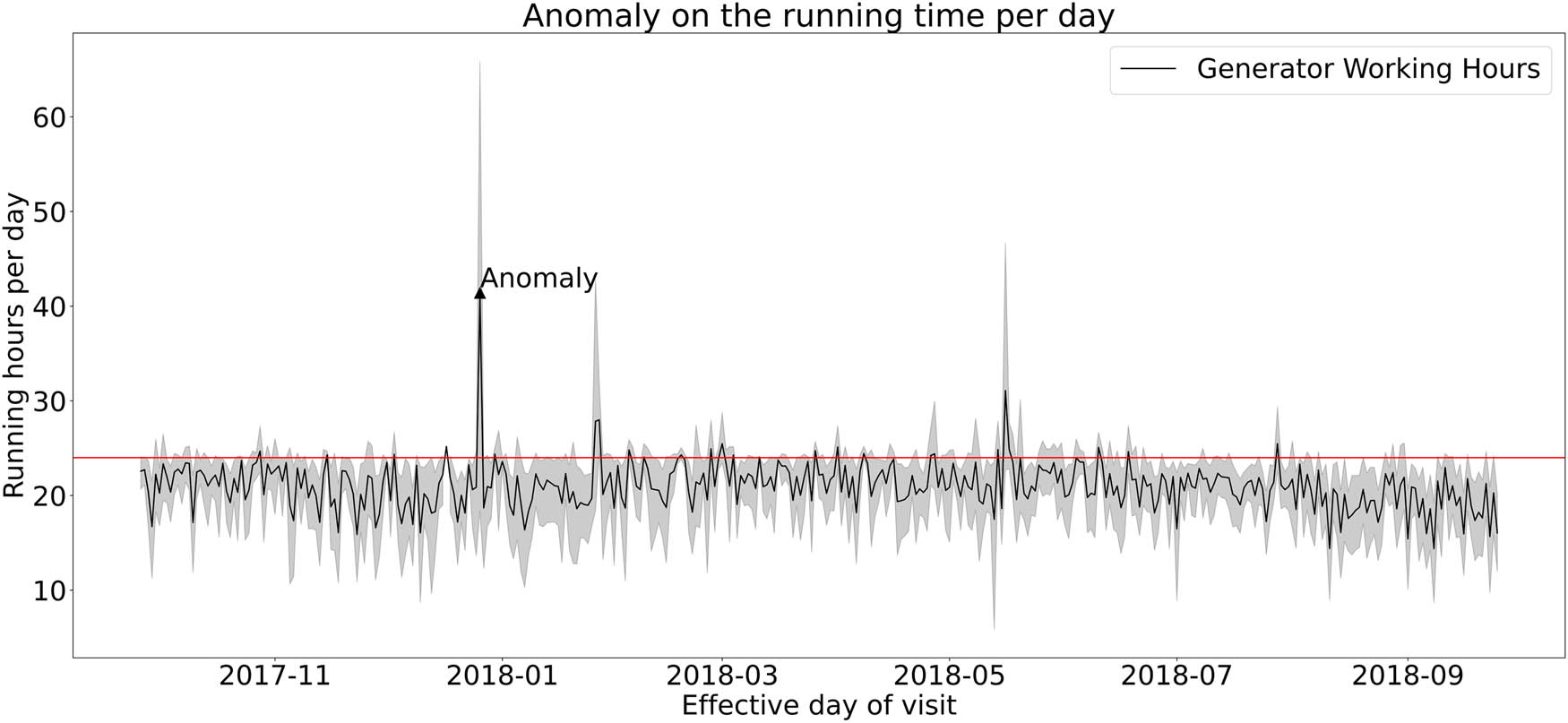
Observed anomaly in the number of working hours in a day for a single generator. For example, all data samples above the 24 h threshold show anomalies in the running time of the generator, and these samples are assigned label 1 because it is known that 1 day only has 24 h.

Figure 3

Fuel consumed per cluster showing the degree of anomalies in the dataset.

3.1.2 Feature importance

Feature selection is performed by fitting the data using a RF classifier with 16 features. Note that one could use any other method to find the most important feature. Since the relative importance of the most important feature is too high (100% as shown in Figure 4) compared to other features, any algorithm will predict the same feature as the most important. Figure 4 shows that the feature Running time per day has the greatest influence on the output and can be coined as the most important feature in the dataset. Even though it is followed by the Daily consumption within a period, the huge difference between the Running time per day and the remaining features shows that priority should be given to the feature Running time per day when considering its reconstruction error for anomaly detection.

Figure 4

Feature importance for the 16 variables fitted using RF classifier. The feature Running time per day has the greatest influence on the output and can be coined as the most important feature in the dataset.

3.1.3 Correlation

The correlation matrix is used to visualize the linear relationship between two variables. The values produced by the covariance matrix range from − 1 to 1, where 1 indicates a strong positive linear relationship, − 1 indicates a strong negative linear relationship, and 0 indicates that there is no linear relationship between the variables. Figure 5 shows that the key variable Running time per day and the variable Daily consumption within a period have a strong positive correlation, which is reasonable since the daily quantity of fuel consumed by a generator is a function of the running time. A strong correlation is also observed between the three pairs of features: Total quantity of fuel after refilling, Quantity of fuel found, and the Previous quantity of fuel recorded. However, the feature Previous hour meter G1 has no significant correlation with any of the features.

Figure 5

Correlation matrix of all numerical features. The Running time per day and Daily consumption within a period have a strong positive correlation, which is reasonable since the daily quantity of fuel consumed by a generator is a function of the running time.

3.2 Ensemble learning models

RF is an ensemble learning method used in machine learning that operates by constructing several decision trees at the training phase. The individual trees are then aggregated to produce a more accurate and stable prediction [25]. The gradient boosted decision trees (GBDT) construct a model progressively, focusing on improving a specific loss function. Initially, it starts with a basic prediction model. Then, each step works to reduce the loss by adjusting for the errors of the previous model. This is done by fitting a decision tree to these errors and determining the best rate at which to incorporate this new tree into the model. With each iteration, the model becomes more refined by adding the new tree’s output, adjusted by a learning rate that controls the influence of each tree. This iterative process continues until the model reaches the desired level of accuracy or completes a predefined number of steps [26,27]. XGBoost enhances GBDT by integrating regularization terms into its objective function. This integration effectively controls model complexity, leading to improved performance and generalization capabilities [28]. CatBoost enhances GBDT by introducing the ordered target statistic method for categorical features, which sorts values based on their correlation with the target, allowing for effective encoding and improved model understanding. In addition, CatBoost processes textual features by converting them into uniform-length vectors through feature hashing, and then merging these vectors to capture better feature correlations and interactions [29,30].

LightGBM stands out from XGBoost with innovative tree construction and data processing approaches, focusing on histogram-based learning and leaf-wise tree growth [31]. Unlike XGBoost’s level-wise strategy, LightGBM adopts a leaf-wise growth approach, strategically creating splits for the most significant loss reduction, resulting in more balanced trees. The histogram technique discretizes features into bins, enhancing computational efficiency during tree building, which is particularly beneficial for extensive datasets. This leaf-wise growth contribute to LightGBM’s efficiency and scalability. It excels at handling large datasets and complex models, making it preferable for applications requiring swift model training and processing substantial data volumes. AdaBoost is based on GBDT, aiming to enhance the decision trees’ performance by iteratively adjusting the weights of incorrectly classified instances. In AdaBoost, each instance in the dataset is initially assigned an equal weight, ensuring an unbiased starting point for the selection process. The algorithm then proceeds through a series of iterations, each time training a weak tree classifier on the weighted instances to minimize the error in classification [32,33].

3.3 The architecture of the proposed autoencoder, training, and testing phases

A label-assisted module is integrated into an autoencoder [34]. This process enhances the autoencoder’s functionality by using labelled data for improved feature representation and learning efficiency.

The encoder takes high-dimensional input data, a fixed-size vector, and reaches the latent space by mapping it to a low-dimensional representational vector. The decoder reconstructs the input data from the reduced representation in the latent space. The final reconstruction error is used to set a threshold to detect anomalies. An additional computation block is added to check from a set of labelled data if the threshold is acceptable to satisfy the required precision. This kind of validation block uses the threshold to decide if the threshold should be changed or if the autoencoder should be trained to minimize the reconstruction loss further. The entire architecture of the proposed assisted autoencoder is depicted in Figure 6, and a detailed description is provided as follows:

The dataset, X , comprises observations and features, resulting in a two-dimensional array of size N × M , where N and M represent the number of features and the number of observations, respectively. All features of each observation are collected and received as input in the algorithm called nodes.
The input data of size N × M are collected and reduced to a latent form of size N × Q , where Q < M , while the N × Q set is fed into the decoder to produce a predicted output of size N × M . Appendix A shows the parameters and the architecture of the deep neural networks trained in the encoder and decoder. The encoding and decoding phases display the number of filters, size of filters, and layers.
After decoding, a reconstruction error is produced for each data point. The reconstruction error refers to the measure of how much the reconstructed input deviates from the original input. A threshold is set as a decision point to decide the acceptable deviation amount, and the observation features that go beyond this threshold are classified as an anomaly. The observation below this threshold is normal data without anomaly.
The label assisting module then takes over to verify if each of the observations is labelled, and then the label is used to verify the veracity of the corresponding anomaly classification. The labelled observations are then checked, and an agreement is reached if the threshold is satisfied to obtain the desired precision to detect anomalies; if not, the threshold is updated, or the model is further trained to find the best hyperparameters for the given threshold.

Figure 6

Overview of the proposed model. Each observation goes through the autoencoder for training, the reconstruction error is measured, and then a threshold is used to decide whether the observation is an anomaly. The labelling assistance module then takes over to check if each of the observations is labelled, and then the label is used to check the veracity of the corresponding anomaly classification. A consensus is then reached on whether training should stop, whether the threshold should be updated, or the training should continue with the search for hyperparameters.

To illustrate the aforementioned steps, an example of a scenario is described as follows. Assume the input data X : , i is an observation with N features, and their corresponding predictions are given as follows:

(1) X : , i = X 1 , i , X 2 , i , X 3 , i , … , X N − 1 , i , X N , i ,

(2) = ( 0.1 , 0.2 , 0.3 , … , 0.4 , 0.5 ) ,

(3) X ˆ : , i = X ˆ 1 , i , X ˆ 2 , i , X ˆ 3 , i , … , X ˆ N − 1 , i , X ˆ N , i ,

(4) = ( 0.6 , 0.21 , 0.32 , … , 0.61 , 0.53 ) .

The value of each feature indicates the feature’s importance in the anomaly classification; e.g., the running time of a generator is more important than the generator capacity. The reconstruction loss for each feature is then calculated:

(5) L : , i = ∣ X : , i − X ˆ : , i ∣ ,

(6) = ( 0.5 , 0.01 , 0.02 , 0.21 , 0.03 ) .

Assume the maximum reconstruction loss is set to 0.2, then the absolute error classifies the sample under the normal category while if a priority is given to the important feature, say X N − 1 , i , then the sample would be labelled as an anomaly since the reconstruction loss of X N − 1 , i is L N − 1 , i = 0.21 , which is beyond 0.2 . Figure 7 illustrates the reconstruction loss scenario adopted in this example. Both the training and testing phases are equally important when it comes to the generalization of the model. The dataset is divided into training and testing, depending on the proportion of choice; in our case, we used the ratio of 3:1 for training and testing, respectively. The training phase is divided into two folds. First, minimizing the reconstruction error is the focus of the training for the reconstructed outputs to converge to the input samples. Second, the reconstruction error is calculated for each data point to find an optimal threshold for anomaly detection.

$Figure 7 Computing reconstruction loss for X : , i = ( X 1 , i , X 2 , i , X 3 , i , … , X N − 1 , i , X N , i ) {{\bf{X}}}_{:,i}=\left({{\bf{X}}}_{1,i},{{\bf{X}}}_{2,i},{{\bf{X}}}_{3,i},\ldots ,{{\bf{X}}}_{N-1,i},{{\bf{X}}}_{N,i}) using the predicted output X ˆ : , i = ( X ˆ 1 , i , X ˆ 2 , i , X ˆ 3 , i , … , X ˆ N − 1 , i , X ˆ N , i ) {\hat{{\bf{X}}}}_{:,i}=\left({\hat{{\bf{X}}}}_{1,i},{\hat{{\bf{X}}}}_{2,i},{\hat{{\bf{X}}}}_{3,i},\ldots ,{\hat{{\bf{X}}}}_{N-1,i},{\hat{{\bf{X}}}}_{N,i}) .$

Figure 7

Computing reconstruction loss for X : , i = ( X 1 , i , X 2 , i , X 3 , i , … , X N − 1 , i , X N , i ) using the predicted output X ˆ : , i = ( X ˆ 1 , i , X ˆ 2 , i , X ˆ 3 , i , … , X ˆ N − 1 , i , X ˆ N , i ) .

The training phase consists of normalizing the dataset, so that all the features are reduced to a common scale without distorting the differences in the range of the values. In this work, the mathematical measure used to normalize the data is given by:

(7) X : , iscaled = X : , i − X : , min X : , max − X : , min ,

where X : , min and X : , max represent the data point with the minimum and maximum entries, respectively. This is followed by dividing and separating the anomalous samples from the training set so that the algorithm learns to reconstruct the norms. Once the training is completed, a reconstruction loss between the input and output is calculated, and a backpropagation strategy is applied to adjust the weights and parameters of the model. The testing phase checks the performance of the model on the unseen test data using the threshold obtained from the training phase. The whole process is described in Figure 7.

3.4 Performance metrics

Performance metrics are essential for assessing the overall quality of a model. Since a single metric cannot fully validate a model’s effectiveness, a combination of metrics, including accuracy, F1 score, recall, precision, and specificity, are used to evaluate the models discussed in this article. The confusion matrix as shown in Table 2 generates more meaningful measures to find the detection accuracy, precision, recall, and F1 score. True normal (TN) represents the number of observations in the normal class that are predicted as normal by the model (i.e., below the threshold). True anomaly (TA) is the number of observations in the anomaly class that are predicted as an anomaly and are above the threshold. False normal (FN) is the number of anomalous observations that are below the threshold (i.e., predicted as normal classes). False Anomaly (FA) is the number of normal observations that are above the threshold (i.e. predicted as an anomaly).

Table 2

Two class classification confusion matrix representation

Classification class distribution
	Actual normal	Actual anomaly
Predicted normal	True normal	False normal
Predicted anomaly	False anomaly	True anomaly

The classification accuracy measures the general performance of the model by producing the ratio of true prediction (true normal and true anomaly) out of the total number of predictions:

(8) Accuracy = TN + TA TA + TN + FA + FN .

The precision is the ratio of the true anomaly divided by the total number of observations above the threshold (i.e., the number of anomalies predicted):

(9) Precision = TA TA + FA .

The false positive rate (FPR) refers to the ratio of the normal samples above the threshold to the actual number of normal samples:

(10) FPR = FA FA + TN .

True positive rate (TPR), also known as sensitivity or recall, is the ratio of the number of anomalous samples above the threshold to the actual number of samples in the anomaly class:

(11) TPR = TA TA + FN .

Specificity is the ratio of true normal to the total negative class in the sample:

(12) Specificity = TN TN + FA .

F 1 score gives the harmonic mean between recall and precision of the classifier. A high F1 score indicates a better performance of the classifier with no false alarm:

(13) F 1 score = 2 Precision × Recall Precision + Recall .

4 Experimental results and analysis

We present the results obtained from training and testing the discussed classifiers. Our analysis includes a comparative study against existing works using the same datasets presented in the studies by Mulongo et al. [5] and Atemkeng and Jimoh [8].

4.1 Training

The data are split into 75% training and 25% testing sets, respectively. To assess the performance of our model during training, we set aside 10% of the training data to validate the model. The training and validation losses trend down different epochs for all the classifiers. We noticed rapid learning for the ensemble learning models, suggesting the potential for early stopping around epoch 10. These ensemble learning models’ training losses and validation curves are asymptotic, indicating generalization capability. We observe that the label-assisted autoencoder’s validation loss is below the training loss as shown in Figure 8. However, this can not influence the predicted accuracy with further hyperparameter tuning since the difference between the two errors is negligible. Finding the label-assisted autoencoder appropriate threshold requires testing the model with the entire test dataset. The confusion matrix is used to determine the model’s accuracy and TPR. They are plotted over a range of thresholds as shown in Figure 9 (top-panel) and the level at which they both attain an average maximum point is the best threshold for the model. The Training Accuracy (depicted by the red line) indicates the training accuracy, whereas the Predicted Anomaly (shown by the blue line) reflects the model’s predicted performance on the training data. We note that, at a threshold of 0.0, the training accuracy is approximately 30%, and the Predicted Anomaly is 100%. Conversely, at a threshold of 1.0 or above, the training accuracy increases to roughly 70%, while the Predicted Anomaly decreases to below 10%. The most effective training threshold identified is 0.232, at which both the Training Accuracy and the Predicted Anomaly converge to an approximate value of 96%. However, if the sensitivity (TPR) or predicted anomaly is a priority for the organization without minding the cost they may secure while sorting out the False normal (predicted anomalies that are actually), the threshold could then be reduced to 0.231. This is the point where all anomalies are predicted (i.e., predicted anomalies are at 100%) with a higher false normal (FN), which has an effect on the overall model accuracy. The threshold is also used to categorize these anomalies from mild to extreme using their reconstruction error. Figure 9 (bottom panel) shows the reconstruction error. Here, 0 denotes normal data, and the value 1 indicates an anomaly. This figure shows that the samples with extreme thresholds are prioritized when one seeks to find the reasons for the presence of anomalies.

Figure 8

Training and validation loss as a function of the number of iterations. The mean absolute error is used to measure the loss.

Figure 9

Threshold detection (top panel) using the reconstruction error (bottom panel). The threshold is used to categorize anomalies from mild to extreme using their reconstruction error. In the bottom panel, the legend with 0 means normal, and 1 means an anomaly.

4.2 Model performance

The total number of test samples is 1,476, with 1,006 normal samples and the remaining 470 anomalous samples.

Figure 10 illustrates the performance of the proposed label-assisted autoencoder model with a threshold of 0.232 (left panel) and 0.231 (right panel) based on the confusion matrix. The proposed model is able to detect a total of 455 anomalous samples correctly out of the 470 samples with the anomaly label, and this accounts for 96.8% (TPR) of the total anomaly samples. The model also detected a total number of 979 normal samples correctly out of 1,006. The model incorrectly classified 15 normal samples as anomalies (FN) and 27 anomalies as normal samples (FA). These results show an accuracy of 97.15%, a precision of 94.40%, a recall of 96.81%, a specificity of 97.31%, and an F1 score of 95.59%. Table 3 presents a summary of the performance metrics. Figure 11 shows the confusion matrices for each ensemble learning model. All ensemble learning models demonstrated a high true normal rate, effectively classifying the normal class. Similarly, they exhibited a high true anomaly rate, accurately identifying anomalies. Conversely, these models showed a low false normal rate, indicating a reduced likelihood of misclassifying anomalies as normal. A low false anomaly rate also suggests that normal instances are rarely incorrectly labelled as anomalies. This performance indicates a robust ability of the ensemble models to distinguish between normal and anomalous classes accurately. In terms of accuracy, F1 score, recall, precision, and specificity, we observe the following:

AdaBoost: Accuracy of 99.4%, F1 score of 99.1%, recall of 98.9%, precision of 99.3%, and specificity of 99.7%.
CatBoost: Accuracy of 99.4%, F1 score of 99.1%, recall of 98.5%, precision of 99.7%, and specificity of 99.9%.
RF: Accuracy of 99.4%, F1 score of 99.1%, recall of 98.7%, precision of 99.5%, and specificity of 99.8%.
LightGBM: Accuracy of 99.6%, F1 score of 99.4%, recall of 99.1%, precision of 99.7%, and specificity of 99.9%.
XGBoost: Accuracy of 99.7%, F1 score of 99.5%, recall of 99.1%, precision of 100%, and specificity of 100%.
GBDT: Accuracy of 99.7%, F1 score of 99.6%, recall of 99.5%, precision of 99.7%, and specificity of 99.9%.

Figure 10

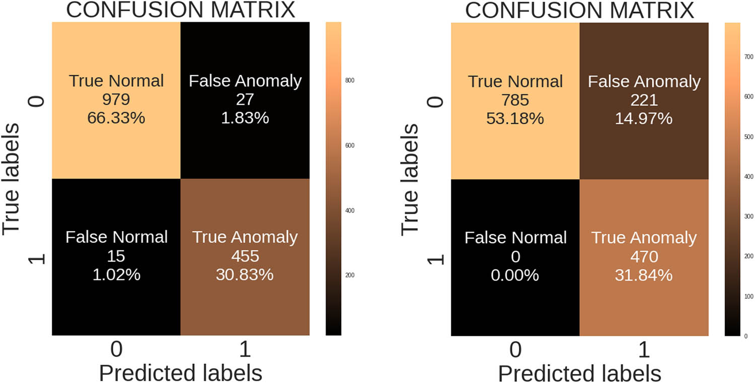
Confusion matrices for the label-assisted autoencoder with a threshold of 0.232 (left panel) and 0.231 (right panel).

Table 3

The performance evaluation for the label-assisted AE demonstrates how the performance metrics are a function of the autoencoder threshold

Model performance
Threshold	Accuracy	F1 score	Recall	Precision	Specificity
0.232	0.972	0.956	0.968	0.944	0.973
0.231	0.850	0.810	1.00	0.680	0.780

Figure 11

Confusion matrices for each ensemble learning models: AdaBoost (top-left), CatBoost (top-right), RF (middle-left), LightGBM (middle-right), XGBoost (bottom-left), and GBDT (bottom-right).

Table 4 shows the performance of the proposed models compared to that discussed in Mulongo et al. [5] and Atemkeng and Jimoh [8]. We used the latter papers to compare our work because both are implemented using the same Teneifera dataset for anomaly detection. The proposed label-assisted autoencoder has the best performance with an accuracy of 97.2% and a recall of 96.8% compared to the MLP proposed in Mulongo et al. [5], while the F1 score of the MLP shows the most competitive performance with a higher F1 score, specificity, and precision. However, the label-assisted autoencoder is flexible since if we adjust the threshold, the recall will increase at the cost of specificity and overall accuracy. Also, the GAN proposed in Atemkeng and Jimoh [8] demonstrated superior performance compared to the label-assisted autoencoder. This can be attributed to the data augmentation capability inherent in GANs.

Table 4

Comparison of the autoencoder and ensemble learning models with models used in the literature and trained on the identical dataset reveals notable insights into anomaly detection performance

Model performance
Paper	Techniques	Accuracy	F1-Score	Recall	Precision	Specificity
[5]	LR	0.708	0.811	0.709	0.943	0.699
	SVM	0.949	0.962	0.962	0962	0.925
	KNN	0.851	0.888	0.887	0.890	0.783
	MLP	0.961	0.971	0.954	0.988	0.976
[8]	GANs	0.989	0.645	0.796	0.785	Not provided in [8]
Autoencoder (AE)	Label-AE	0.972	0.956	0.968	0.944	0.973
Ensemble learning	AdaBoost	0.994	0.991	0.989	0.993	0.997
	CatBoost	0.994	0.991	0.985	0.997	0.999
	RF	0.994	0.991	0.987	0.995	0.998
	LightGBM	0.996	0.994	0.991	0.997	0.999
	XGBoost	0.997	0.995	0.991	1.0	1.0
	GBDT	0.997	0.996	0.995	0.997	0.999

While all ensemble learning models demonstrated superior performance compared to the label-assisted autoencoder and the works by Mulongo et al. and Atemkeng and Jimoh [5,8], GBDT and XGBoost exhibited the highest performances. Nevertheless, there remains significant value in using autoencoders. Autoencoders offer the unique capability of assessing anomaly accuracy based on severity, a feature inaccessible to ensemble learning models. This nuanced approach allows for a more granular understanding of anomaly detection, enhancing the overall effectiveness of the detection process. Feature importance played an important role in training the autoencoder. The feature Running time per day has the most significant importance of 100, and Daily consumption within a period comes in the second place with an important measure of 16; from this, we gave priority to the reconstruction error of the Running time per day. To further justify our choice, the correlation matrix in Figure 5 shows a strong positive correlation of 0.74 between the two features. By using the reconstruction error of the key variable, we were able to train and compare the proposed autoencoder with the work by Mulongo et al. [5]. A recall score of 96.8% outperformed all the models proposed by Mulongo et al. [5] in detecting anomalies. Also, as shown in Table 3, our model shows a recall score of approximately 100% with a decrease in the overall accuracy of 85% when the threshold is decreased to 0.231.

4.3 Autoencoder-based anomaly severity categorization

The reconstruction error for each data sample differs from one another (as shown in Figure 9, bottom panel) and provides an opportunity to classify these predicted anomalies according to their reconstruction error. This work considers four classes A, B, C, and D. Class A represents anomalies that are slightly above the threshold, class B represents anomalies that are above twice the threshold, class C represents anomalies that are above four times the threshold, and class D represents anomalies that are above eight times the threshold. This implies that each class has twice a threshold compared to its predecessor. Table 5 shows the classes and their corresponding thresholds, showing that 28.25% of the test dataset belongs to the anomaly category of class A, 2.03% belongs to class B, 0.20% belongs to class C, and 0.34% belongs to D.

Table 5

Categorizing anomalies with label-assisted autoencoder

Categorizing anomalies
Class	Threshold	Predicted number of samples	Percentage of test data (%)
A	0.232	417	28.25
B	0.464	30	2.03
C	0.928	3	0.20
D	1.856	5	0.34

5 Conclusion

The telecommunication industry is one of the dominant information communication technology industries that rely on a huge amount of electric power supply for their operations, and thus, it is indispensable in their daily dealings. However, its availability in underdeveloped countries, particularly in Africa, has been a constant source of contention. Despite the industry’s rise through the creation of base stations, they have had to turn to alternative energy sources, such as gasoline or diesel with generators and solar power, to name a few.

TeleInfra telecommunication company, established in Cameroon, is one of the companies that are hooked on these challenges due to the state of power supply in the country. The telecommunication equipment that is fixed in different parts of the rural and urban areas in Cameroon requires an uninterrupted supply of electricity to achieve the goal of establishing strong and seamless communication channels in the country. However, the country’s electrical generation is mostly based on hydropower (73%), with perpetual power interruptions, particularly during the dry seasons when water levels are low [35]. The consequence of the diversification to alternative sources of power, particularly the usage of generators, posed another challenge of irregularities or anomalies in fuel consumption at the base stations due to the observed high consumption rate in the power generation plants. TeleInfra telecommunication company is faced with the challenge of unaccounted high fuel consumption for their operations at the base stations. Since they solely depend on generating plants as their major source of power supply, they have to refill these generators continually, and these are done manually. Such activities are known to have emanated in possible cases of pilferage of fuel due to the observed anomalies in fuel consumption. As a result, it is essential to investigate the likely factors contributing to the anomalies by collecting data on fuel consumption at each base station to minimize the operation costs.

This study explored the effectiveness of ensemble learning models for anomaly detection in power generation plants. To achieve this, we examined six different ensemble learning models and observed that all of them proved effective in detecting anomalies. Furthermore, our results indicated that these ensemble learning models outperformed both MLP and GANs, which were initially proposed in the literature for anomaly detection using the same dataset employed in our study.

We also proposed a label-assisted autoencoder-based deep-learning technique for detecting anomalies in the fuel consumption datasets of the base station management company, namely, TeleInfra. In the proposed model, an autoencoder is used to generate an encoded representation of the input features and construct the output from the encoded representation to look like the input features of the series of decoders. The maximum reconstruction error from the trained model is obtained from the training set, and it is set as a threshold for detecting anomalies on the test dataset. The anomaly detector identifies each data sample from the testing set as an anomaly when it exceeds the threshold assigned. Results showed that the autoencoder is highly efficient for reading anomalies with a detection accuracy of 97.20%

This work opens future research possibilities, which could involve using different variations of autoencoders, such as LSTM autoencoders and memory-augmented autoencoders combined with our proposed label-assisted unit. The latter does not require feature importance analysis to select the best reconstruction error. Also, we believe that expanding our investigation to include models such as ResNet, AlexNet, MobileNet, EfficientNet, and others could be a valuable avenue for future research, especially when dealing with larger datasets.

Acknowledgments

We thank the reviewers for their valuable comments, which have significantly enhanced the quality of the article. MA and SH thank Rhodes University for their financial support.

Funding information: Marcellin Atemkeng thanks the National Research Foundation of South Africa for support through project number CSRP23040990793.
Author contributions: Conceptualization: Marcellin Atemkeng; methodology: Marcellin Atemkeng, Victor Osanyindoro, Rockefeller Rockefeller, Sisipho Hamlomo, Jecinta Mulongo, Theophilus Ansah-Narh, Franklin Tchakounté, and Arnaud Nguembang Fadja; software: Marcellin Atemkeng, Victor Osanyindoro, and Rockefeller Rockefeller; validation: Marcellin Atemkeng, Victor Osanyindoro, Rockefeller Rockefeller, Sisipho Hamlomo, Jecinta Mulongo, Theophilus Ansah-Narh, Franklin Tchakounté, and Arnaud Nguembang Fadja; data curation: Marcellin Atemkeng, Victor Osanyindoro, and Jecinta Mulongo; data analysis: Marcellin Atemkeng, Victor Osanyindoro, Rockefeller Rockefeller, Sisipho Hamlomo, Jecinta Mulongo, Theophilus Ansah-Narh, Franklin Tchakounté, and Arnaud Nguembang Fadja; writing – original draft preparation: Marcellin Atemkeng and Victor Osanyindoro; writing – review and editing: Marcellin Atemkeng, Victor Osanyindoro, Rockefeller Rockefeller, Sisipho Hamlomo, Jecinta Mulongo, Theophilus Ansah-Narh, Franklin Tchakounté, and Arnaud Nguembang Fadja; funding: Marcellin Atemkeng.
Conflict of interest: The authors have no conflicts of interest to declare. All coauthors have read and agree with the contents of the manuscript, and there is no financial interest to report.
Ethical approval: Not applicable, as the study did not involve the use of identifiable humans or animals, and thus did not require ethical clearance.
Data availability statement: The datasets generated during and/or analyzed during the current study are available from the corresponding author on reasonable request.

Appendix

The architecture of deep neural networks trained in the encoder and decoder. The number of filters and the size of the filters and layers are displayed in the encoding and decoding phases (Figure A1).

Figure A1

Architecture of the deep neural networks trained in the encoder and decoder.

References

[1] Humar I, Ge X, Xiang L, Jo M, Chen M, Zhang J. Rethinking energy efficiency models of cellular networks with embodied energy. IEEE Network. 2011;25(2):40–9. 10.1109/MNET.2011.5730527Search in Google Scholar

[2] Lorincz J, Bule I. Renewable energy sources for power supply of base station sites. Int J Business Data Commun Network (IJBDCN). 2013;9(3):53–74. 10.4018/jbdcn.2013070104Search in Google Scholar

[3] Ayang A, Ngohe-Ekam PS, Videme B, Temga J. Power consumption: base stations of telecommunication in sahel zone of cameroon: typology based on the power consumption model and energy savings. J Energy. 2016;2016(1):3161060.10.1155/2016/3161060Search in Google Scholar

[4] Espadafor FJ, Villanueva JB, Garciiia MT. Analysis of a diesel generator crankshaft failure. Eng Failure Anal. 2009;16(7):2333–41. 10.1016/j.engfailanal.2009.03.019Search in Google Scholar

[5] Mulongo J, Atemkeng M, Ansah-Narh T, Rockefeller R, Nguegnang GM, Garuti MA. Anomaly detection in power generation plants using machine learning and neural networks. Appl Artif Intel. 2020;34(1):64–79. 10.1080/08839514.2019.1691839Search in Google Scholar

[6] Jinggang W, Ligai K, Meixia D, Jin Z, Xiaoxia G. Feasibility analysis using natural source cooling the IDC plant. In: 2009 Chinese Control and Decision Conference. IEEE; 2009. p. 2579–84. 10.1109/CCDC.2009.5191830Search in Google Scholar

[7] Goodfellow I, Bengio Y, Courville A. Deep learning. Cambridge, Massachusetts, USA: MIT Press; 2016. Search in Google Scholar

[8] Atemkeng M, Jimoh TA. Anomaly detection in power generation plants with generative adversarial networks. In: 2023 International Conference on Electrical, Computer and Energy Technologies (ICECET). IEEE; 2023. p. 1–6. 10.1109/ICECET58911.2023.10389251Search in Google Scholar

[9] Aggarwal CC. An introduction to outlier analysis. In: Outlier analysis. Springer International Publishing; 2017. p. 1–34. 10.1007/978-3-319-54765-7_1Search in Google Scholar

[10] Demestichas K, Alexakis T, Peppes N, Adamopoulou E. Comparative analysis of machine learning-based approaches for anomaly detection in vehicular data. Vehicles. 2021;3(2):171–86. 10.3390/vehicles3020011Search in Google Scholar

[11] Hayes MA, Capretz MA. Contextual anomaly detection framework for big sensor data. J Big Data. 2015;2(1):1–22. 10.1186/s40537-014-0011-ySearch in Google Scholar

[12] Fahim M, Sillitti A. Anomaly detection, analysis and prediction techniques in iot environment: A systematic literature review. IEEE Access. 2019;7:81664–81. 10.1109/ACCESS.2019.2921912Search in Google Scholar

[13] Trinh HD, Zeydan E, Giupponi L, Dini P. Detecting mobile traffic anomalies through physical control channel fingerprinting: A deep semi-supervised approach. IEEE Access. 2019;7:152187–201. 10.1109/ACCESS.2019.2947742Search in Google Scholar

[14] Omar S, Ngadi A, Jebur HH. Machine learning techniques for anomaly detection: an overview. Int J Comput Appl. 2013;79(2):33–41. 10.5120/13715-1478Search in Google Scholar

[15] Vishwanathan S, Murty MN. SSVM: a simple SVM algorithm. In: Proceedings of the 2002 International Joint Conference on Neural Networks. IJCNN’02 (Cat. No. 02CH37290). vol. 3. IEEE; 2002. p. 2393–8. 10.1109/IJCNN.2002.1007516Search in Google Scholar

[16] Peterson LE. K-nearest neighbor. Scholarpedia. 2009;4(2):1883. 10.4249/scholarpedia.1883Search in Google Scholar

[17] Nick TG, Campbell KM. Logistic regression. In: Ambrosius WT, editor. Topics in Biostatistics. Methods in Molecular Biology™. Vol 404. Humana Press; 2007. p. 273–301. 10.1007/978-1-59745-530-5_14.Search in Google Scholar PubMed

[18] Ruck DW, Rogers SK, Kabrisky M. Feature selection using a multilayer perceptron. J Neural Netw Comput. 1990;2(2):40–8. Search in Google Scholar

[19] Bhattacharyya S, Jha S, Tharakunnel K, Westland JC. Data mining for credit card fraud: A comparative study. Decision Support Syst. 2011;50:602–13. 10.1016/j.dss.2010.08.008Search in Google Scholar

[20] Hasan M, Islam MM, Zarif MII, Hashem M. Attack and anomaly detection in IoT sensors in IoT sites using machine learning approaches. Internet Things. 2019;7:100059. 10.1016/j.iot.2019.100059Search in Google Scholar

[21] Said Elsayed M, Le-Khac NA, Dev S, Jurcut AD. Network anomaly detection using LSTM based autoencoder. In: Proceedings of the 16th ACM Symposium on QoS and Security for Wireless and Mobile Networks; 2020. p. 37–45. 10.1145/3416013.3426457Search in Google Scholar

[22] Hawkins S, He H, Williams G, Baxter R. Outlier detection using replicator neural networks. In: International Conference on Data Warehousing and Knowledge Discovery. Springer; 2002. p. 170–80. 10.1007/3-540-46145-0_17Search in Google Scholar

[23] Zhang J, Zhang H, Ding S, Zhang X. Power consumption predicting and anomaly detection based on transformer and K-means. Front Energy Res. 2021;9:681. 10.3389/fenrg.2021.779587Search in Google Scholar

[24] Münz G, Li S, Carle G. Traffic anomaly detection using k-means clustering. In: GI/ITG Workshop MMBnet. vol. 7; 2007. p. 9. Search in Google Scholar

[25] Rodriguez-Galiano V, Sanchez-Castillo M, Chica-Olmo M, Chica-Rivas M. Machine learning predictive models for mineral prospectivity: An evaluation of neural networks, random forest, regression trees and support vector machines. Ore Geol Rev. 2015;71:804–18. 10.1016/j.oregeorev.2015.01.001Search in Google Scholar

[26] Freund Y, Schapire RE. A decision-theoretic generalization of on-line learning and an application to boosting. J Comput Syst Sci. 1997;55(1):119–39. 10.1006/jcss.1997.1504Search in Google Scholar

[27] Freund Y, Schapire RE. Experiments with a new boosting algorithm. In: Machine Learning: Proceedings of the Thirteenth International Conference, 1996. vol. 96. Citeseer; 1996. p. 148–56. Search in Google Scholar

[28] Chen T, Guestrin C. Xgboost: A scalable tree boosting system. In: Proceedings of the 22nd ACm Sigkdd International Conference on Knowledge Discovery and Data Mining; 2016. p. 785–94. 10.1145/2939672.2939785Search in Google Scholar

[29] Hancock JT, Khoshgoftaar TM. CatBoost for big data: an interdisciplinary review. J Big Data. 2020;7(1):94. 10.1186/s40537-020-00369-8Search in Google Scholar PubMed PubMed Central

[30] Prokhorenkova L, Gusev G, Vorobev A, Dorogush AV, Gulin A. CatBoost: unbiased boosting with categorical features. Advances in neural information processing systems. 2018. p. 31. Search in Google Scholar

[31] Ke G, Meng Q, Finley T, Wang T, Chen W, Ma W, et al. Lightgbm: A highly efficient gradient boosting decision tree. 31st Conference on Neural Information Processing Systems, NIPS; 2017. p. 30.Search in Google Scholar

[32] Hastie T, Rosset S, Zhu J, Zou H. Multi-class AdaBoost. Stat Interface. 2009;2(3):349–60. 10.4310/SII.2009.v2.n3.a8Search in Google Scholar

[33] Rätsch G, Onoda T, Müller KR. Soft margins for AdaBoost. Machine Learn. 2001;42:287–320. 10.1023/A:1007618119488Search in Google Scholar

[34] Zhai J, Zhang S, Chen J, He Q. Autoencoder and its various variants. In: 2018 IEEE International Conference on Systems, Man, and Cybernetics (SMC). IEEE; 2018. p. 415–9. 10.1109/SMC.2018.00080Search in Google Scholar

[35] Muh E, Amara S, Tabet F. Sustainable energy policies in Cameroon: A holistic overview. Renew Sustainable Energy Rev. 2018;82:3420–9. 10.1016/j.rser.2017.10.049Search in Google Scholar

Received: 2023-11-28

Accepted: 2024-06-25

Published Online: 2024-11-06

This work is licensed under the Creative Commons Attribution 4.0 International License.

Articles in the same Issue

https://doi.org/10.1515/jisys-2023-0283

Keywords for this article

electric grid; fuel consumption; autoencoder; anomaly detection; power generating plants; GANs; ensemble learning

Creative Commons

BY 4.0