Cross-dataset micro-expression identification based on facial ROIs contribution quantification
-
Kun Yu
 and
Chunfeng Guo
and
Chunfeng Guo

Abstract
In this work, we propose a novel cross-dataset micro-expression identification method based on facial regions of interest contribution quantification, where the training samples are from the source dataset and the test samples are from the target dataset. Specifically, a micro-expression video clip (i.e., a sample) is first sampled at intervals to capture an image sequence consisting of multiple consecutive video frames. Then, locate and crop the facial area in the image frame, and perform facial landmark detection on the cropped area. Next calculate the optical-flow field of the image sequence, and extract the improved Main Directional Mean Optical-flow feature. Finally, the learned group sparse model is used as the classifier to predict the label information of the unmarked target samples, so as to complete the category recognition of micro-expressions. Extensive cross-dataset comparative experiments on four spontaneous micro-expression datasets, CASME, CASME II, SMIC-HS, and SAMM, show that the recognition strategy proposed in this work is effective. Compared with several other advanced recognition methods, our method has better cross-dataset recognition performance, not only the classification accuracy is higher, but also the classification stability is better when faced with different target datasets and different micro-expression categories. It can be applied in many fields such as clinical diagnosis, interrogation, negotiation, and national security.
1 Introduction
Expression is an intuitive reflection of human emotional state, which can usually be divided into macro-expression and micro-expression. In the past few years, the research on facial expression recognition in academia has mainly focused on macro-expressions [1]. Micro-expressions are small, quick, and unconscious facial movements that humans involuntarily reveal when experiencing mood swings and trying to mask their inner emotions, which are special in that they can neither be camouflaged nor forcibly suppressed [2]. Therefore, micro-expressions can be used as a reliable basis for analyzing and judging people’s real psychological emotions, and have strong practical value and application prospects in clinical diagnosis, negotiation, teaching evaluation, polygraph detection, and interrogation.
The duration of micro-expressions is very short, less than half a second [3]. The magnitude of facial muscle movements caused by micro-expressions is very small, occurring only in a few smaller localized facial regions, and usually not on both the upper and lower halves of the human face. These factors make micro-expressions difficult to be observed by the human eye, and the accuracy of manual recognition is not high. In addition, manual recognition of micro-expressions requires professional training and rich classification experience, which is time-consuming and labor-intensive, and is difficult to promote and apply on a large scale in real-world scenarios. Based on the large demand of society and the advancement of technology, in recent years, the use of computer vision and pattern recognition technology to realize the automatic identification of micro-expressions is increasingly attracting the attention of researchers [4,5].
The process of micro-expression automatic recognition can be divided into two stages [6]: The first is to extract micro-expression features, that is, to extract useful feature information from facial video clips; the second is to classify micro-expressions, which uses classifiers to determine the emotion category to which each extracted feature belongs. Most micro-expression recognition research focuses on the feature extraction part, aiming to effectively describe the subtle changes in facial muscles by designing reliable micro-expression features.
The features that have been proposed in recent years to describe micro-expressions can be roughly divided into three categories:
Appearance-based features
As an extension to the Local binary pattern (LBP) feature, LBP from Three Orthogonal Planes (LBP-TOP) is a typical appearance-based feature [7]. Pfister et al. introduced LBP-TOP into micro-expression recognition for the first time [8], using it as a spatiotemporal descriptor to describe the facial micro-expressions in video clips, and proved its effectiveness and its superiority to human eye observation through experiments.
Since then, some researchers have adopted different techniques to improve LBP-TOP or to design spatiotemporal descriptors more suitable for micro-expression recognition. Ruiz-Hernandez and Pietikäinen adopted reparameterization of second-order Gaussian jet to enhance LBP-TOP and obtained satisfactory recognition results on a micro-expression database [9]. Wang et al. used Robust Principal Component Analysis (RPCA) to extract background information from micro-expression video clips, and then adopted LBP-TOP and Local Spatiotemporal Directional Features for micro-expression recognition [10]. They also proposed a color space decomposition method based on Tensor Independent Color Space, which decomposes micro-expression samples into different color channels, and uses color information for micro-expression recognition [11,12]. Wang et al. proposed to use six intersection points to reduce the redundant information of LBP-TOP, and developed a variant feature of LBP-TOP, called LBP with six intersection points (LBP-SIP) [13], the experimental results show that the recognition effect of LBP-SIP is better than that of LBP-TOP. Huang et al. proposed a spatiotemporal descriptor using an image integral operation projection technique, called Spatiotemporal LBP with integration projection (STLBP-IP) [14], to describe micro-expressions. Experimental results show that STLBP-IP outperforms popular spatiotemporal descriptors such as LBP-TOP and LBP-SIP in terms of recognition rate. Subsequently, Huang et al. introduced local structural information into LBP-TOP and proposed Spatiotemporal Completed Local Quantization Patterns (STCLQP) [15]. STCLQP divides a video clip into several blocks, and concatenates the respective features in all blocks into an overall feature. But obviously the feature dimension of STCLQP is very high.
Optical-flow-based features
Common to this class of features is the estimation and computation of optical-flow in video.
Liu et al. proposed a Main Directional Mean Optical-flow (MDMO) feature [16]. According to the Facial Action Coding System (FACS) [17], the entire face is divided into 36 regions of interest (ROIs). The histograms of oriented optical flow (HOOF) feature of each ROI is calculated separately to determine its principal direction. The principal directions of all ROIs are combined into a 72-dimensional feature vector. Finally, the feature vector is averaged in the time dimension to obtain the MDMO feature.
Another representative feature based on optical-flow is the Facial Dynamics Map (FDM) proposed by Xu et al. [18], which can characterize the movement of micro-expressions in different granularities. First, pixel-level alignment of micro-expression image sequences is performed by estimating optical-flow, and then each micro-expression image sequence is divided into several spatiotemporal cuboids according to granularity. The principal optical-flow direction of each cuboid is calculated using an iterative method in order to represent the local facial dynamics. Combining all these principal optical-flow directions, a FDM representing an image sequence of micro-expression can be obtained.
MDMO and FDM features are two typical spatiotemporal descriptors under non-LBP frameworks, both of which take advantage of special properties in micro-expressions to optimize the estimated optical-flow, making it insensitive to illumination changes.
Deep-learning-based features
In recent years, deep learning techniques have also been used to deal with the problem of micro-expression recognition. For example, Kim et al. combined the popular and excellent convolutional neural network (CNN) and Long short-term memory (LSTM) recurrent neural network [19] to learn deep features for describing micro-expressions. Under this deep learning framework, a representative expression state frame of a micro-expression video clip is first selected to train a CNN. Then, the CNN features of each image frame in the video clip are extracted and used to train the LSTM network to recognize micro-expressions. It is worth noting that since deep learning relies heavily on large-scale datasets, the vast majority of deep features currently do not exceed traditional features in terms of recognition rate.
In summary, the research on micro-expression automatic recognition based on image analysis has achieved some beneficial results. Although these studies still have considerable room for improvement in terms of recognition accuracy and real-time performance, they still achieve a recognition effect far superior to human eye perception, and explore the technical route of micro-expression automatic recognition from different angles.
It should be pointed out that the development of micro-expression recognition research largely relies on a well-established facial micro-expression dataset. Currently publicly available micro-expression datasets mainly include: CASME [20,21] and CASME II [22] datasets from the Institute of Psychology, Chinese Academy of Sciences, SMIC dataset [23] from the University of Oulu, Finland, SAMM dataset [24,25] from Manchester Metropolitan University, UK, Polikovsky dataset [26] from the University of Tsukuba, Japan, and USF-HD dataset [27] from the University of South Florida, USA.
Micro-expressions have specific occurrence scenarios. Strictly speaking, micro-expressions simulated subjectively by humans are not real micro-expressions. Therefore, the induction method directly determines the authority and reliability of the micro-expression dataset. When filming, CASME, CASME II, SMIC, and SAMM all require subjects (i.e., participants) to try their best not to show their inner emotions when watching stimulating videos or materials that can cause emotional fluctuations. And a reward and punishment mechanism is used to motivate subjects to suppress their emotions and avoid being discovered by the recorder, thereby ensuring the reliability of the generated micro-expressions. Meanwhile, other micro-expression datasets only allowed the subjects to perform directly or imitate the micro-expressions in the video according to the requirements of the collector. Considering that CASME, CASME II, SMIC, and SAMM are all spontaneously generated, this study selects these four datasets as research objects.
The above four micro-expression datasets were all elicited in well-controlled laboratory environment, and appropriate lighting was used to eliminate light flickering.
By reviewing the previous research work, it can be found that most of the existing micro-expression recognition methods are developed and evaluated under the condition that the training samples and test samples come from the same dataset, and the training samples and test samples follow the same or similar feature distribution. But obviously, in real-world applications, training samples and test samples often come from two completely different micro-expression datasets, and the video clips in these two datasets will be different in terms of lighting conditions, shooting equipment, parameter settings, and background environments. Therefore, in this case, due to the heterogeneous video quality, the training samples and test samples will be very different, making their feature distribution also have great differences, resulting in a significant reduction in the recognition effect of most current micro-expression recognition methods.
In this study, we try to solve this challenging and realistic problem, and develop a practical cross-dataset micro-expression recognition scheme that can adapt to complex application scenarios. For convenience, the dataset to which the training samples belong is referred to as the source dataset, and the dataset to which the test samples belong is referred to as the target dataset. We assume that the sample label information of the source dataset is known, while the samples of the target dataset are all unlabeled. Therefore, the core research content of this study is the problem of unsupervised cross-dataset micro-expression recognition.
2 Overall design idea
In this study, we conduct specialized studies for the case where the training samples and test samples belong to two different datasets, and thus propose a novel cross-dataset micro-expression identification method based on facial ROIs contribution quantification (FRCQ).
Specifically, a micro-expression video clip (i.e., a sample) is first sampled at intervals, thereby capturing an image sequence consisting of multiple consecutive video frames. Considering that the efficiency of the recognition algorithm will be reduced if the size of the image frame is too large, the image frame is down-sampled.
Then, locate and crop the facial region in an image frame, and perform facial landmark detection on the cropped region image. Based on these obtained key points and facial Action units (AU) theory, a face is divided into 36 ROIs. Since redundant frames will affect the recognition accuracy, a temporal interpolation model (TIM) is used to normalize the number of frames in the image sequence. Next we compute the optical-flow field of the image sequence and extract our improved MDMO feature.
Considering that the training samples and test samples belong to different datasets, the distribution status of their MDMO feature data is often quite different. We draw on the ideas of domain adaptation and domain regeneration based on transfer component analysis, and use the transfer learning method to perform feature transformation on the test samples in the target dataset (referred to as target samples), so that their reconstructed MDMO features follow the same feature distribution law as the training samples in the source dataset (referred to as source samples). According to the MDMO features of the source samples and their marked label information, we iteratively learn and build a group sparse model, in order to filter out those ROIs that are truly associated with micro-expression actions and can help distinguish micro-expression categories, and specifically quantify the contribution of each facial ROI to micro-expression formation. At last, the learned group sparse model is used as the classifier to predict the label information of the unmarked target samples, so as to realize micro-expression recognition.
The cross-dataset micro-expression identification algorithm based on FRCQ is shown in Figure 1.
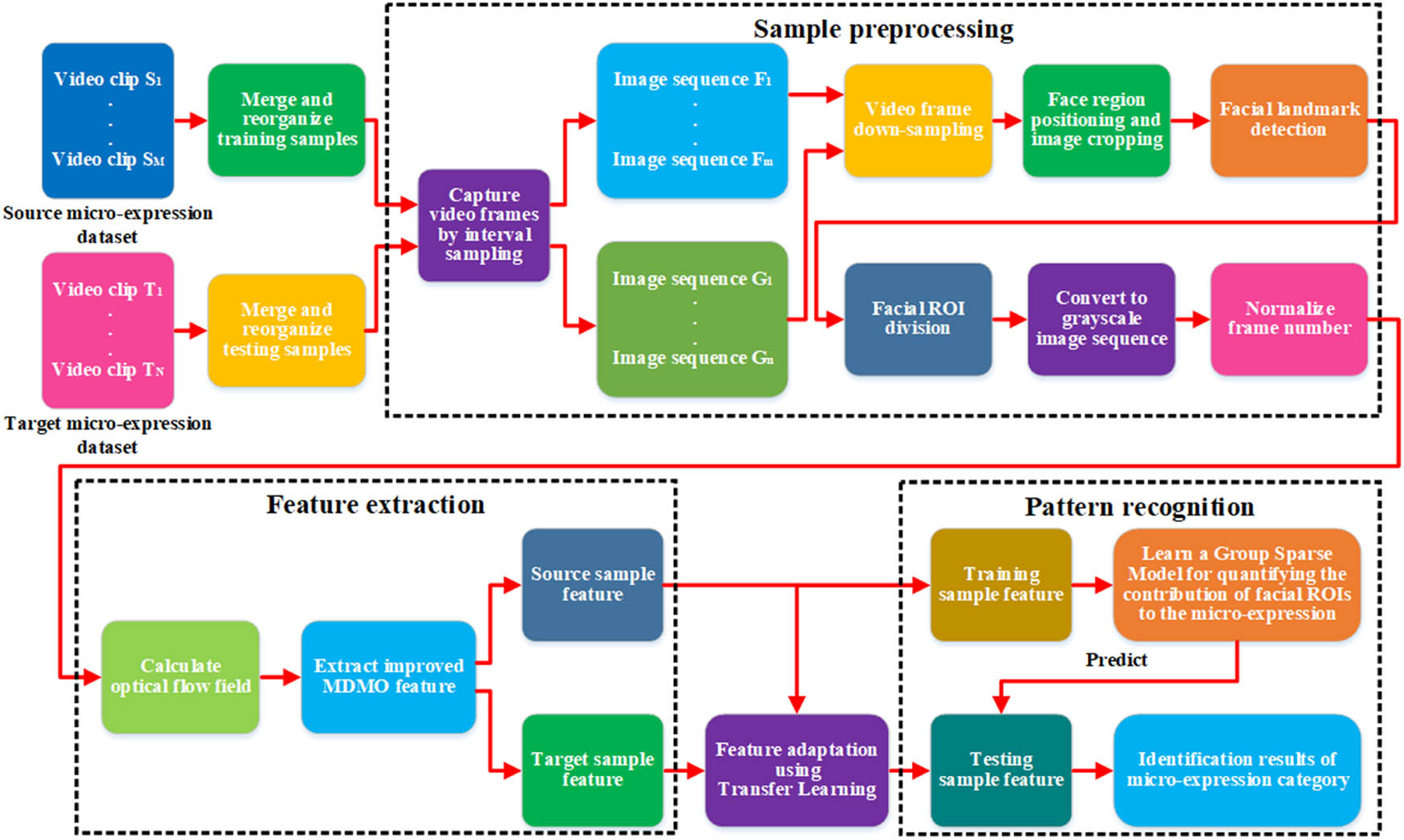
Flowchart of cross-dataset micro-expression identification algorithm based on FRCQ.
3 Micro-expression sample preprocessing
The micro-expression recognition process for micro-expression datasets includes three steps in turn: sample preprocessing, feature extraction, and pattern recognition. In this study, sample preprocessing mainly includes image sequence generation, video frame down-sampling, facial region localization and facial image cropping, facial landmark detection, facial ROI division, image sequence graying, and frame number normalization of an image sequence, etc.
A sample in the micro-expression dataset refers to a complete micro-expression video clip with a certain emotion, including three important frames: Onset frame, apex frame, and offset frame. Among them, onset refers to the moment when the micro-expression begins to appear, apex refers to the moment when the micro-expression has the largest amplitude, and offset refers to the moment when the micro-expression disappears. Taking these three special moments as interval points, the occurrence time of a micro-expression can be divided into two stages, as shown in Figure 2.

Examples of sample video clips in the form of image sequences from four spontaneous micro-expression datasets. The micro-expressions from top to bottom are surprise, happiness, positive, and anger. Since the apex frames are not marked in the SMIC dataset, the frame at the intermediate moment is given at the corresponding position in the figure. (a) CASME, (b) CASME II, (c) SMIC, and (d) SAMM. Source: The facial photos in the figure are from four spontaneous micro-expression datasets (CASME, CASME II, SMIC and SAMM).
3.1 Image sequence generation
The micro-expression video clips are first converted into image sequences. For a micro-expression video clip Γ, several consecutive still images, namely, video frames, are intercepted from the video clip by setting the sampling interval.
Since the devices that shoot micro-expression videos are all high-speed cameras, the video frame rate is very high, but the massive image frames contained in the video clips are not all conducive to micro-expression analysis, so the number of redundant frames can be reduced by interval sampling.
Assuming that the original frame rate is m frames/second (Frames Per Second, FPS), and the video duration is t vid seconds, then the video has a total of m × t vid frames. If the sampling period is t sam seconds, then the corresponding number of frames is m × t sam, which means that one frame is extracted every m × t sam frames. In this way, only [t vid/t sam] frames are included in the resulting image sequence, where [] is an integer-valued function.
Since the four micro-expression datasets used in this study all provide image sequences of video clips, in the following experiments, these given image sequences are directly used as samples.
3.2 Video frame down-sampling
Different micro-expression datasets have different sizes of video images, which makes it impossible for subsequent operations to be performed at the same scale. For this reason, and also to reduce computational complexity, we down-sample video frames in all sample image sequences based on bicubic interpolation. Resize the video frame width uniformly to 500 pixels and keep the original aspect ratio.
3.3 Facial region localization and facial image cropping
Face alignment is a common preprocessing step in face recognition and macro-expression recognition. However, we found that face alignment can lead to a certain degree of facial deformation, which undoubtedly has a large negative impact on micro-expressions that are originally very low in intensity, and even directly buries small facial muscle changes. Therefore, traditional face alignment is not performed in this study.
In fact, since the duration of a micro-expression is short enough that the magnitude of head displacement (including translation and rotation) in successive multiple frames of each image sequence is so small that it can be ignored. We adopt the face detector proposed by Masayuki Tanaka [28] to perform face detection only on the first frame of each image sequence, in order to locate the face region. This detection algorithm can not only detect multiple frontal faces appearing in the same image with high accuracy, but also detect their corresponding left eye, right eye, mouth, and nose at the same time. Even when the input image is rotated or the head is tilted in the image, the detection effect is still excellent.
It should be pointed out that this algorithm can only detect images with three color channels, while the SAMM dataset provides grayscale image sequences with one color channel, so in practice, we convert all of them into three-channel form.
In addition, after extensive experiments, we found that there are differences in lighting conditions, background complexity, subjects’ skin color, and facial shape in different datasets, which make the face detection algorithm under the same parameter setting unable to accurately locate facial regions of all sample image sequences. For example, there may be a missing part of the chin in the detected face region. To solve this problem, we take the center point of the original rectangular bounding box as the benchmark, and expand the rectangular box in all sample image sequences to the surrounding area according to the same proportion to ensure that the size of the facial area is appropriate. Figure 3 shows the front face and facial organ detection results of some samples presented in the form of rectangular bounding boxes on four micro-expression datasets.

Front face and facial organ detection results for the first frame of sample image sequences from four spontaneous micro-expression datasets. Among them, the detected front face, left eye, right eye, nose, and mouth are located in green, blue, magenta, yellow, and cyan bounding boxes, respectively. (a) CASME, (b) CASME II, (c) SMIC, and (d) SAMM. Source: The facial photos in the figure are from four spontaneous micro-expression datasets (CASME, CASME II, SMIC and SAMM).
For each image sequence, according to the position and size of the facial region detected in the first frame, the corresponding regions of all frames are cropped to form a new facial image sequence.
3.4 Facial landmark detection using discriminative fitting of response map (DFRM) algorithm
We adopt a texture model-dependent DFRM algorithm [29] to achieve high-accuracy facial landmark detection. This algorithm filters the image using a set of filters, producing sparse response maps that are used to build texture models. Each filter is separately trained according to its respective texture model in order to locate a specific landmark point. As mentioned earlier, we only detect the first frame in each facial image sequence in order to obtain 66 feature points that describe the key locations of the face. Figure 4 shows examples of facial landmark detection using the DFRM algorithm on four micro-expression datasets, where the red “+” marks represent the detected key feature points.
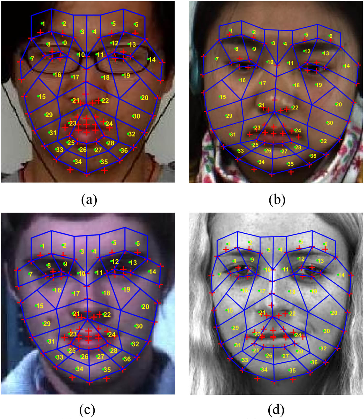
Examples of facial landmark detection and ROI division based on DFRM algorithm and FACS on four spontaneous micro-expression datasets. Among them, the red “+” markers represent the detected facial key feature points, a total of 66. The green “.” markers represent the centroid of each facial ROI, a total of 36. The yellow number is the number of the facial ROI. Each ROI is surrounded by four vertices connected in pairs, and adjacent ROIs are separated by blue lines. (a) CASME, (b) CASME II, (c) SMIC, and (d) SAMM. Source: The facial photos in the figure are from four spontaneous micro-expression datasets (CASME, CASME II, SMIC and SAMM).
3.5 Facial ROI division
There are various strategies for the division of facial ROIs, but the general principle is that it can neither be too dense nor too sparse. If the division is too dense, redundant information may be introduced; if the division is too sparse, useful information may be missed.
Since micro-expressions only involve the contraction or relaxation of local facial muscles, we further divide the facial region into 36 specific non-overlapping but closely adjacent ROIs by using the coordinates of key feature points obtained by the DFRM algorithm, while excluding some irrelevant regions, as shown in Figure 4. The location and size of these ROIs are uniquely determined by 66 feature points, which are divided according to the facial AU in the FACS [17]. In other words, each ROI corresponds to some AUs, which can fully reflect the apparent changes produced by facial muscle movements. The combination of all ROIs can represent almost all types of micro-expressions.
Given that color information in color images is susceptible to illumination, we grayscale all sample image sequences. Subsequent processing will be performed on the grayscale image sequences, which can also speed up feature extraction.
3.6 Frame number normalization for image sequences
The number of frames contained in different sample image sequences often varies greatly; and the number of frames will affect the quality of subsequent feature extraction to a certain extent: too few frames will limit the extraction of certain types of spatiotemporal texture feature descriptors (such as LBP-TOP), and too many frames will introduce a lot of redundant information irrelevant to micro-expression recognition.
Therefore, we normalize the number of frames per sample using the TIM proposed by Zhou et al. [30]. Compared with linear interpolation [16], which obtains a fixed number of frames, this TIM-based video length normalization technique interpolates the required number of frames from the low-dimensional manifold structure established by the facial image sequence, which is obviously more flexible and reasonable.
4 Improved MDMO feature extraction
For the preprocessed sample image sequence, we first calculate its optical-flow field, and then extract the improved optical-flow-based MDMO feature to meet the needs of quantifying the contribution of the facial ROIs.
4.1 Optical-flow field calculation
Optical flow is the instantaneous moving speed of the pixels corresponding to a spatially moving object on the imaging plane. The optical-flow vector refers to the instantaneous change rate of the gray level of a specific pixel on a two-dimensional image plane. By analyzing the changes in the optical flow vectors of the pixels between two frames of an image sequence, the spatial position correspondence between the two frames can be determined, thereby estimating the movement information of objects in the image.
The optical-flow field is a two-dimensional vector field, which reflects the gray level change trend of each pixel on the image, and contains the vector information of the instantaneous moving speed and direction of each pixel. It can be viewed as the instantaneous velocity field generated by the movement of pixels with grayscale on the image plane. This movement can be caused by either the camera or an object.
For the micro-expression recognition task using datasets recorded in well-controlled laboratory scenarios, the optical flow can only be caused by human movement due to the stationary camera used for filming. Therefore, we expect to quantitatively estimate the motion of the subject’s facial muscles in a micro-expression video clip as precisely as possible by computing the optical-flow field of the corresponding grayscale image sequence.
There are many methods that can be used to calculate the optical-flow field. The basic principle is to calculate the difference between two frames by encoding the moving speed and direction of each pixel from one frame and another. This study adopts the Robust Local Optical Flow algorithm based on the Hampel estimator proposed by Senst et al. [31].
In practice, for a micro-expression image sequence (f 1, f 2, …, f m ) with m frames captured by a high-speed camera, the changes between two adjacent frames are very small, and the presented optical flow changes are not very obvious.
Therefore, we calculate the optical flow vector [V x , V y ] between each frame f i (i > 1, except the first frame) and the first frame f 1, where V x and V y are the components of the optical-flow velocity; and then convert the coordinates in Cartesian form to polar form (ρ, θ), where ρ and θ are magnitude and angle, respectively.
4.2 Improved MDMO feature
MDMO feature [16] is a standardized feature that counts the optical-flow information in the ROI, and its most notable advantage is that its feature dimension is small.
Since both local motion statistics and spatial locations are considered, MDMO feature is consistent for ROIs at the same location in image sequences of different faces exhibiting the same category of micro-expression, and MDMO feature is good at distinguishing the movements of facial muscles under different micro-expression states.
Suppose there is a micro-expression video clip Γ containing m frames, i.e., an image sequence (f 1, f 2, …, f m ). As mentioned earlier, the facial region in each frame is divided into 36 ROIs by 66 landmark points. Calculate the optical flow vector between each frame f i (i > 1) and the first frame f 1.
In each frame f
i
(i > 1), all optical-flow vectors in each ROI
Calculate the average of all the optical-flow vectors belonging to B
max, and define it as the main direction optical flow of
MDMO represents each frame f i (i > 1) by an atomic optical-flow feature Ψ i
The dimension of Ψ i is 36 × 2 = 72. An m-frame micro-expression video clip Γ can be represented as a set of atomic optical-flow features
Take the average of
The above equation expresses the average of the main direction optical flow vectors of the ROIs at the same position (all are the kth ROIs) of all frames (starting from the second frame) in the current video clip, so as to obtain the main direction average optical-flow vector of the kth ROI.
This gives a 72-dimensional vector
Considering that the magnitudes of the main directions in different video clips may vary greatly, further normalizes the magnitudes in the vector
Replace
It should be pointed out that, unlike the approach in [16], we do not decompose the normalized MDMO feature into amplitude and angle parts, nor introduce a trade-off parameter to balance the amplitude and angle parts. Instead, take
In Section 6, we will use the group sparse model to assign a weight to each ROI to specifically quantify the contribution of the MDMO feature of the facial region to the formation of micro-expressions. For example, if the weight is 0, it means that its corresponding facial ROI has little contribution to the occurrence of micro-expressions.
5 Target sample feature adaptation using transfer learning
When training samples and test samples come from different micro-expression datasets, the distribution states (mainly the data probability distribution, including the mean and variance, etc.) of MDMO feature data extracted from the same ROI using the same method are often quite different, which makes the direct use of traditional machine learning methods to construct classifiers for pattern recognition not ideal.
To address this issue, we employ a transfer learning approach to narrow the feature distribution differences in different data domains. We draw on the idea of domain adaptation based on transfer component analysis in the study by Pan et al. [32] and domain regeneration in the study by Zong et al. [33], and perform feature transformation on the test samples (referred to as target samples) in the target dataset, so as to obtain new reconstructed MDMO features that satisfy the same feature distribution rules as the training samples (referred to as source samples) in the source dataset. The source sample features remain unchanged; the newly generated target sample features still retain the discrimination of the original features, but enhance the adaptability to the established model.
The following describes the target sample feature adaptation algorithm based on transfer learning. It is assumed here that the label information of the target samples is all unknown, and the feature structure of the target samples needs to be transformed according to the feature distribution characteristics of the source sample.
Suppose
The feature of the source samples should remain unchanged during this process, i.e., the following condition needs to be met:
(7)where G is the feature transformation operator of the target samples.
After G transforms the features of the target samples, the new reconstructed features of the target samples and the features of the source samples should have the same or similar distribution characteristics. A function
where λ is the weight coefficient used to adjust the balance of the two terms in the objective function.
The feature transformation operator G of the target samples can be designed through kernel mapping and linear projection operations.
Specifically, the source samples are first projected from the original feature space to the Hilbert space through a kernel mapping operator
To eliminate the feature distribution difference between the source and target samples, their maximum mean discrepancy (MMD) distance within the Hilbert space can be minimized. Therefore, MMD can be regarded as the regular term
where H represents the Hilbert space, 1
s
and 1
t
are column vectors of length n
s
and n
t
, respectively, with all l elements. However, directly taking MMD as
It can be shown that minimizing MMD in equation (10) is equivalent to minimizing
Substituting
Let
where
6 Learning a group sparse model to quantify the contribution of facial ROIs to micro-expressions
In the previous sample preprocessing step, we divided the entire face region into 36 ROIs, but in fact
Not every ROI plays a role in the occurrence of micro-expressions. This is because the occurrence of micro-expressions only involves a small part of the face area, and the facial muscles in many ROIs are almost completely motionless during this period, making the optical flow generated by them very weak. Therefore, the MDMO feature data extracted in these ROIs not related to micro-expression recognition can be considered as invalid or redundant information.
The number and location of ROIs related to different types of micro-expressions are not the same; and for the same type of micro-expressions, the roles played by each ROI also vary.
Based on the above considerations, we hope to be able to filter out those ROIs that are truly associated with micro-expression actions and help distinguish micro-expression categories, and specifically quantify their contribution to micro-expressions.
Considering that the classification model based on sparse representation has strong advantages in machine learning and pattern recognition, and can effectively solve problems such as overfitting in high-dimensional data modeling, we decided to learn a sparse representation model to quantify the contribution of each facial ROI.
Aiming at the local sparsity and non-local self-similarity of face images, the sparse representation unit we choose is a group, and each group is composed of the MDMO feature matrix of a certain facial ROI. Specifically, we build a group sparse model based on 72-dimensional MDMO features from 36 facial ROIs and their micro-expression label information.
Assuming that there are M micro-expression training samples, their corresponding MDMO feature matrix is
l k,j = 1, when the kth sample belongs to the jth category of micro-expression (1 ≤ k ≤ M, 1 ≤ j ≤ c);
l k,j = 0, other cases.
The above label vectors are actually a set of standard orthonormal bases, which can be expanded into a vector space containing label information. Therefore, a projection matrix U can be introduced to establish the relationship between the feature space and the label space of the samples. This projection matrix U can be obtained by solving the following objective function:
The U
T
X in the above equation can be rewritten as
In order to numerically measure the specific contribution of each facial ROI to the occurrence of micro-expressions, we introduce a weighting coefficient β
i
for each ROI in equation (15), and add a non-negative L1 norm
where μ is a trade-off coefficient that determines the number of non-zero elements in the learned weight vector β.
The regularization term in equation (16) has two benefits. First, during model learning, ROIs that hardly contribute to micro-expression recognition will be discarded (its corresponding coefficient β i is 0). Second, each selected ROI will be assigned a positive rational weight to measure its contribution.
To improve the classification performance of the group sparse model, we further extend its linear kernel to a nonlinear kernel. Use the nonlinear mapping
The inner product operation in the kernel space is then replaced by a kernel function. In the kernel space F,
Substitute
where
This work adopts the alternative directional method [34,35] to solve the optimization problem of equation (18), i.e., iteratively updates the values of parameters P and β i until the objective function converges.
7 Micro-expression category recognition for target samples using a group sparse model
For the training samples in the source dataset, after the optimal parameter values
For a test sample, let its feature vector be
where
Assuming that the obtained label vector is
8 Experimental results and discussion
The experiments were programmed using MATLAB R2022B (64-bit) software (MathWorks, Natick, MA, USA) under the Windows 10 operating system (Microsoft, Redmond, WA, USA).
Considering that the categories of micro-expressions in the four datasets are not uniform, and they all have the class-imbalance problems in different degrees, we combined some of the samples according to their categories. The experimental sample information is shown in Table 1.
Experimental sample information of four spontaneous micro-expression datasets
| Dataset | Emotion category | Number of original samples | Combined emotion category | Number of combined samples |
|---|---|---|---|---|
| CASME | Happiness | 10 | Positive | 11 |
| Contempt | 1 | |||
| Disgust | 42 | Negative | 49 | |
| Fear | 2 | |||
| Sadness | 5 | |||
| Repression | 43 | — | — | |
| Tenseness | 71 | — | — | |
| Surprise | 19 | Surprise | 19 | |
| CASME II | Happiness | 32 | Positive | 32 |
| Disgust | 63 | Negative | 69 | |
| Fear | 2 | |||
| Sadness | 4 | |||
| Repression | 27 | — | — | |
| Others | 99 | — | — | |
| Surprise | 28 | Surprise | 28 | |
| SMIC-HS | Positive | 51 | Positive | 51 |
| Negative | 70 | Negative | 70 | |
| Surprise | 43 | Surprise | 43 | |
| SAMM | Happiness | 26 | Positive | 38 |
| Contempt | 12 | |||
| Anger | 57 | Negative | 80 | |
| Disgust | 9 | |||
| Fear | 8 | |||
| Sadness | 6 | |||
| Others | 26 | — | — | |
| Surprise | 15 | Surprise | 15 |
It can be seen from Table 1 that merging samples from datasets with more micro-expression (emotion) categories can not only solve the mismatch problem of micro-expression categories between the source dataset and the target dataset, but also alleviate the class-imbalance problem of samples to a certain extent.
All the merged samples belong to three classes: “Positive,” “Negative,” and “Surprise.” In fact, considering the ambiguity of the micro-expression itself on the classification boundary, it is reasonable for us to divide the micro-expression samples for training and testing into three classes, and such a classification scale is easier to apply in practice.
Positive micro-expressions represent an individual’s “superficially” good emotions, including happiness and contempt. Negative micro-expressions reflect that an individual is in a bad mood, including disgust, fear, sadness, and anger. Surprised micro-expressions occur when there is a discrepancy between expectations and reality, without obvious, strong emotional overtones and directionality, and are usually classified as a separate class. Repression and tenseness indicate a person’s ambiguous feelings, which can be either neutral, positive or negative, and need to be further inferred in combination with the scene, so we eliminated these two categories of micro-expressions in the experiment. The samples of the “Others” category contain many uncertain emotions, so they are also discarded in the experiment.
8.1 Influence of the number of frames on recognition effect
In order to observe the influence of the number of frames in the sample image sequence on the micro-expression recognition effect, we adopted facial ROIs contribution quantification algorithm proposed in this study to conduct cross-dataset micro-expression recognition experiments under three conditions:
The number of original frames,
The number of frames normalized by linear interpolation [16],
The number of frames normalized by the TIM [30].
Figure 5 presents part of the experimental results in the form of confusion matrix

Cross-dataset micro-expression recognition results from SMIC-HS to SAMM with different numbers of frames. The overall recognition accuracy from left to right is 45.87, 41.35, and 51.13%, respectively. (a) The number of original frames, (b) the number of frames normalized by linear interpolation, and (c) the number of frames normalized by the TIM.
In each confusion matrix given in Figure 5, each column represents the predicted category of the feature data, and each row represents the true attribution category of the feature data; the three values on the main diagonal line represent the recognition accuracy of positive, negative, and surprised micro-expression categories under the current frame number, respectively. It can be found that the number of frames normalized by the TIM has a relatively higher recognition accuracy for various micro-expressions, so the experimental effect is the best. In all the experiments, we use the TIM to normalize the number of frames.
8.2 Influence of kernel function on recognition effect
When performing transfer learning on the target sample features, we introduce the kernel function. Figure 6 shows the effect of different types of kernel functions on the micro-expression recognition performance.
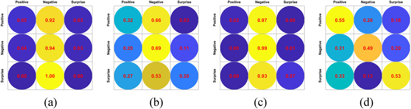
The effect of using different kernel functions in transfer learning on the experimental results of cross-dataset micro-expression recognition from SMIC-HS to SAMM. (a) Polynomial kernel function, (b) Gaussian kernel function, (c) chi-square kernel function, and (d) linear kernel function.
Figure 6 clearly shows that the linear kernel function produces the best result. Therefore, this study adopts the linear kernel function to realize the feature adaptation of the target samples.
When learning the group sparse model, we also introduce the kernel function. Figure 7 shows the effects of different types of kernel functions on the experimental results of micro-expression recognition.

The effect of using different kernel functions in group sparse model learning on the experimental results of cross-dataset micro-expression recognition from SMIC-HS to SAMM. (a) Polynomial kernel function. (b) Gaussian kernel function. (c) Chi-square kernel function. (d) Linear kernel function.
In Figure 7, the Chi-square kernel function produces the best result. Therefore, this study uses the Chi-square kernel function to learn the group sparse model for quantifying the contribution of facial ROI and realizing the category recognition of micro-expressions.
8.3 Two-by-two cross-dataset micro-expression recognition experiment
In order to verify the effectiveness of the cross-dataset micro-expression recognition algorithm based on FRCQ proposed in this study, we conduct extensive pairwise cross-dataset micro-expression recognition experiments on four micro-expression datasets: CASME, CASME II, SMIC-HS, and SAMM. One of the two acts as a source dataset, providing training samples while the other acts as a target dataset, providing test samples.
The FRCQ algorithm is compared with three state-of-the-art micro-expression recognition algorithms, and the experimental results are shown in Figures 8–10. None of the three comparison methods do any transformation on the extracted features, and all use support vector machine (SVM) with polynomial kernel as the classifier.
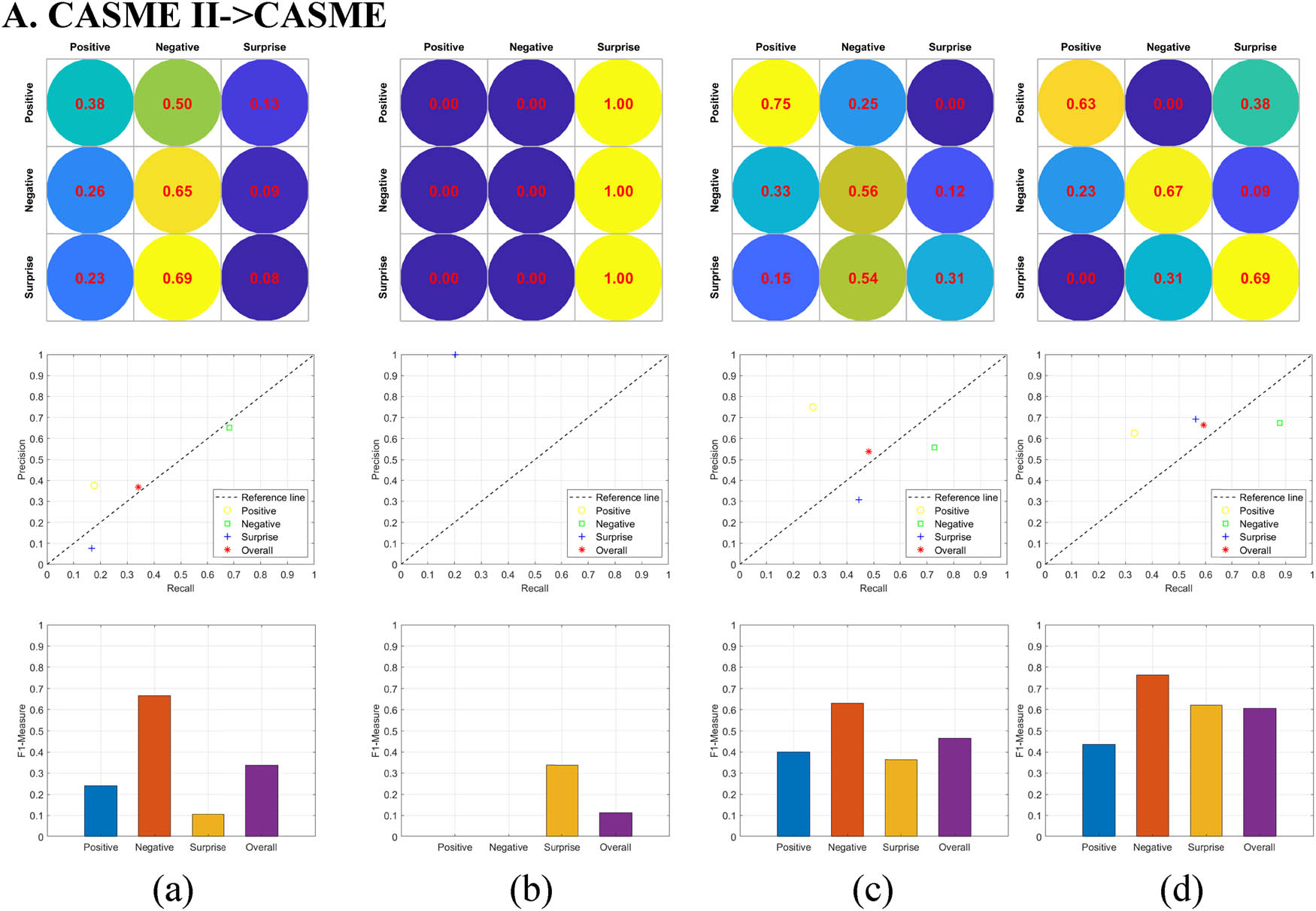
Comparison results of different methods in cross-dataset micro-expression recognition experiments from source dataset CASME II to target dataset CASME. From top to bottom are the confusion matrix, the PR curve in the form of discrete points, and the F1-Measure histogram. The recognition accuracy from left to right is 50, 20.31, 53.13, and 67.19%, respectively. (a) LBP-TOP-Whole + SVM, (b) LBP-TOP-ROIs + SVM, (c) MDMO + SVM, and (d) FRCQ.
Comparison results of different methods in cross-dataset micro-expression recognition experiments from source dataset SMIC-HS to target dataset CASME. From top to bottom are the confusion matrix, the PR curve in the form of discrete points, and the F1-Measure histogram. The recognition accuracy from left to right is 50.00, 46.88, 57.81, and 62.50%, respectively. (a) LBP-TOP-Whole + SVM, (b) LBP-TOP-ROIs + SVM, (c) MDMO + SVM, and (d) FRCQ.

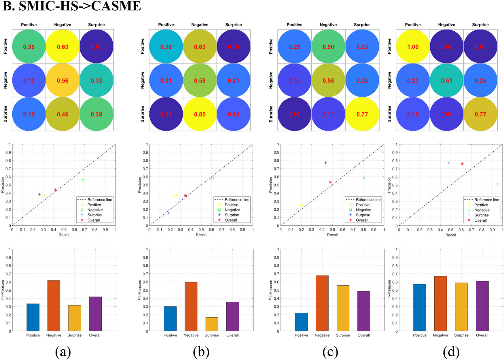
Comparison results of different methods in cross-dataset micro-expression recognition experiments from source dataset SMIC-HS to target dataset CASME II. From top to bottom are the confusion matrix, the PR curve in the form of discrete points, and the F1-Measure histogram. The recognition accuracy from left to right is 22.12, 27.43, 63.72, and 71.68%, respectively. (a) LBP-TOP-Whole + SVM, (b) LBP-TOP-ROIs + SVM, (c) MDMO + SVM, and (d) FRCQ.
Among them, the comparison method 1 extracts the LBP-TOP features of the whole face region (LBP-TOP-Whole + SVM); comparison method 2 extracts the LBP-TOP features of each facial ROI (36 in total) and connects them into combined features (LBP-TOP-ROIs + SVM); and comparison method 3 extracts the original MDMO features of the face (MDMO + SVM).
Due to space limitations, only some of the experimental results are shown here. In the following description, the symbol “A- > B” represents the micro-expression recognition experiment from the source dataset A to the target dataset B.
In the above three sets of comparative experiments, in order to quantitatively compare and analyze the recognition effect of each method, the confusion matrix, the PR curve in the form of discrete points, and the F1-Measure histogram are drawn, respectively, and the overall recognition accuracy of each method is given.
By observing the given confusion matrices, it is not difficult to find that, compared with the advanced “LBP-TOP or MDMO feature + SVM” combination method, the recognition accuracy of our proposed FRCQ method for the three categories of micro-expressions always maintains a high level, and the numerical fluctuation between categories is small. Especially in the two sets of experiments CASME II- > CASME and SMIC-HS- > CASME II, the recognition accuracy of the FRCQ method for the three categories of micro-expressions exceed 60%. In terms of the overall recognition accuracy, the FRCQ method achieves the highest value in its set in all three sets of comparative experiments.
According to the label information of the feature data of the test samples, we plotted the Precision–Recall (PR) curve in the form of discrete points. In the PR curves shown in Figures 8–10, each marker represents the classification result of a micro-expression. For distinction, markers of different shapes and colors are adopted for each category of micro-expression and the overall micro-expression classification results, and a reference line with a slope of 1 is added to the PR curve for easy observation. By comparing the positions of all markers, it can be found that the distribution of the four markers of the FRCQ method is more concentrated than other methods, and is closer to the (1, 1) coordinate point in the upper right corner, which shows that its classification effect is the best.
In order to evaluate the real classification effect more scientifically, we also adopt the F1-Measure evaluation index
The higher the F1 value, the better the classification performance. Using this indicator can easily compare the classification quality of various recognition methods for different micro-expressions.
In the F1-Measure histograms shown in Figures 8–10, the four recognition methods have their own strengths, i.e., each method has its own specific micro-expression categories that is good at classifying. However, except for the FRCQ method, the F1 values of the other three methods are not stable enough and even fluctuate to varying degrees, which shows that they have poor adaptability to the micro-expression image sequences in the target dataset, and the quality of classification presents a certain chance, so they are not suitable for classifying target samples that are quite different from the source samples.
Obviously, the F1 values of the FRCQ method are generally higher than those of the other methods, and always remain at a high level. This shows that the classification quality of the FRCQ method is higher, and the discrimination of small differences in facial detail features is better; the classification performance is more stable and robust, and it can successfully complete the cross-dataset classification task.
9 Conclusion
In this study, we conduct an in-depth study on the cross-dataset micro-expression recognition problem, which is more difficult and challenging than conventional macro-expression and micro-expression recognition, and design an effective micro-expression recognition system based on FRCQ.
For four spontaneous micro-expression datasets, we conduct a large number of cross-dataset micro-expression recognition experiments. The experimental results show that, compared with the other state-of-the-art methods, our FRCQ recognition scheme has achieved the best recognition results in three cross-dataset situations: It not only has a significantly higher recognition accuracy, but also shows strong adaptability and stable classification performance for samples in micro-expression datasets with different characteristics.
Furthermore, in addition to the quality difference between the sample images in the source and target datasets, it can be concluded that the degree of class imbalance in the number of micro-expression samples is also the main factor affecting the difficulty of the cross-dataset micro-expression recognition task.
The micro-expression recognition scheme proposed in this study provides the possibility for real-time automatic analysis of large-scale micro-expression video clips and even practical applications in natural scenes. It has important scientific value and broad application prospects in many fields such as clinical diagnosis, social interaction, and national security.
-
Funding information: This study was supported by the Project of Shandong Province Higher Educational Science and Technology Program (No. J18KA350) in China.
-
Author contributions: Kun Yu proposed design ideas, wrote source code, completed experiments, and wrote this article. Chunfeng Guo organized the experimental data and proofread the manuscript.
-
Conflict of interest: The authors declare no conflict of interest. It should be pointed out that the corresponding author has signed Usage License Agreements with the rights holders of the four micro-expression datasets used in this article.
-
Data availability statement: Four spontaneous micro-expression datasets CASME, CASME II, SMIC-HS and SAMM that can be applied for use by their respective rights holders. Most of the data used in the authors’ research are included in this article, and other data are available from the corresponding author on reasonable request.
References
[1] Zhao X, Zhu J, Luo B, Gao Y. Survey on facial expression recognition: History, applications, and challenges. IEEE Multimed. 2021;28(4):38–44. 10.1109/MMUL.2021.3107862.Search in Google Scholar
[2] Ben X, Ren Y, Zhang J, Wang SJ, Kpalma K, Meng W, et al. Video-based facial micro-expression analysis: A survey of datasets, features and algorithms. IEEE Trans Pattern Anal Mach Intell. 2022;44(9):5826–46. 10.1109/TPAMI.2021.3067464.Search in Google Scholar PubMed
[3] Yan WJ, Wu Q, Liang J, Chen YH, Fu XL. How fast are the leaked facial expressions: the duration of micro-expressions. J Nonverbal Behav. 2013;37(4):217–30. 10.1007/s10919-013-0159-8.Search in Google Scholar
[4] Goh KM, Ng CH, Lim LL, Sheikh UU. Micro-expression recognition: an updated review of current trends, challenges and solutions. Vis Comput. 2020;36(3):445–68. 10.1007/s00371-018-1607-6.Search in Google Scholar
[5] Pan H, Xie L, Wang Z, Liu B, Yang M, Tao J. Review of micro-expression spotting and recognition in video sequences. Virtual Real Intell Hardware. 2021;3(1):1–17. 10.1016/j.vrih.2020.10.003.Search in Google Scholar
[6] Esmaeili V, Mohassel Feghhi M, Shahdi SO. A comprehensive survey on facial micro-expression: approaches and databases. Multimed Tools Appl. 2022;81:40089–134. 10.1007/s11042-022-13133-2.Search in Google Scholar
[7] Zhao G, Pietikainen M. Dynamic texture recognition using local binary patterns with an application to facial expressions. IEEE Trans Pattern Anal Mach Intell. 2007;29(6):915–28. 10.1109/TPAMI.2007.1110.Search in Google Scholar PubMed
[8] Pfister T, Li X, Zhao G, Pietikäinen M. Recognising spontaneous facial micro-expressions. IEEE International Conference on Computer Vision; 2011. p. 1449–56. 10.1109/ICCV.2011.6126401.Search in Google Scholar
[9] Ruiz-Hernandez JA, Pietikäinen M. Encoding local binary patterns using the re-parametrization of the second order Gaussian jet. 10th IEEE International Conference and Workshops on Automatic Face and Gesture Recognition (FG); 2013. p. 1–6. 10.1109/FG.2013.6553709.Search in Google Scholar
[10] Wang SJ, Yan WJ, Zhao G, Fu X, Zhou C. Micro-expression recognition using robust principal component analysis and local spatiotemporal directional features. European Conference on Computer Vision. Cham: Springer; 2014. p. 325–38. 10.1007/978-3-319-16178-5_23.Search in Google Scholar
[11] Wang SJ, Yan WJ, Li X, Zhao G, Fu X. Micro-expression recognition using dynamic textures on tensor independent color space. 22nd IEEE International Conference on Pattern Recognition; 2014. p. 4678–83. 10.1109/ICPR.2014.800.Search in Google Scholar
[12] Wang SJ, Yan WJ, Li X, Zhao G, Zhou CG, Fu X, et al. Micro-expression recognition using color spaces. IEEE Trans Image Process. 2015;24(12):6034–47. 10.1109/TIP.2015.2496314.Search in Google Scholar PubMed
[13] Wang Y, See J, Phan RCW, Oh YH. LBP with six intersection points: Reducing redundant information in LBP-TOP for micro-expression recognition. Asian Conference on Computer Vision; 2014. p. 525–37. 10.1007/978-3-319-16865-4_34.Search in Google Scholar
[14] Huang X, Wang SJ, Zhao G, Pietikäinen M. Facial micro-expression recognition using spatiotemporal local binary pattern with integral projection. Proceedings of the IEEE International Conference on Computer Vision Workshops; 2015. p. 1–9. 10.1109/ICCVW.2015.10.Search in Google Scholar
[15] Huang X, Zhao G, Hong X, Zheng W, Pietikäinen M. Spontaneous facial micro-expression analysis using spatiotemporal completed local quantized patterns. Neurocomputing. 2016;175:564–78. 10.1016/j.neucom.2015.10.096.Search in Google Scholar
[16] Liu YJ, Zhang JK, Yan WJ, Wang SJ, Zhao G, Fu X. A main directional mean optical flow feature for spontaneous micro-expression recognition. IEEE Trans Affect Comput. 2015;7(4):299–310. 10.1109/TAFFC.2015.2485205.Search in Google Scholar
[17] Ekman P, Rosenberg EL. What the face reveals: Basic and applied studies of spontaneous expression using the Facial Action Coding System (FACS). New York, NY, USA: Oxford University Press; 1997. 10.1093/oso/9780195104462.001.0001Search in Google Scholar
[18] Xu F, Zhang J, Wang JZ. Microexpression identification and categorization using a facial dynamics map. IEEE Trans Affect Comput. 2017;8(2):254–67. 10.1109/TAFFC.2016.2518162.Search in Google Scholar
[19] Kim DH, Baddar WJ, Ro YM. Micro-expression recognition with expression-state constrained spatio-temporal feature representations. Proceedings of the 24th ACM International Conference on Multimedia; 2016. p. 382–6. 10.1145/2964284.2967247.Search in Google Scholar
[20] Yan WJ, Wu Q, Liu YJ, Wang SJ, Fu X. CASME database: A dataset of spontaneous micro-expressions collected from neutralized faces. The 10th IEEE International Conference on Automatic Face and Gesture Recognition; 2013. p. 1–7. 10.1109/FG.2013.6553799.Search in Google Scholar
[21] Yan WJ, Wang SJ, Liu YJ, Wu Q, Fu X. For micro-expression recognition: Database and suggestions. Neurocomputing. 2014;136:82–7. 10.1016/j.neucom.2014.01.029.Search in Google Scholar
[22] Yan WJ, Li X, Wang SJ, Zhao G, Liu YJ, Chen YH, et al. CASME II: An improved spontaneous micro-expression database and the baseline evaluation. PLoS One. 2014;9(1):e86041. 10.1371/journal.pone.0086041.Search in Google Scholar PubMed PubMed Central
[23] Li X, Pfister T, Huang X, Zhao G, Pietikäinen M. A spontaneous micro-expression database: Inducement, collection and baseline. The 10th IEEE International Conference on Automatic face and Gesture Recognition; 2013. p. 1–6. 10.1109/FG.2013.6553717.Search in Google Scholar
[24] Davison AK, Lansley C, Costen N, Tan K, Yap MH. SAMM: A spontaneous micro-facial movement dataset. IEEE Trans Affect Comput. 2016;9(1):116–29. 10.1109/TAFFC.2016.2573832.Search in Google Scholar
[25] Davison AK, Merghani W, Yap MH. Objective classes for micro-facial expression recognition. J Imaging. 2018;4(10):119. 10.3390/jimaging4100119.Search in Google Scholar
[26] Polikovsky S, Kameda Y, Ohta Y. Facial micro-expressions recognition using high speed camera and 3D-gradient descriptor. The 3rd International Conference on Imaging for Crime Detection and Prevention; 2009. p. 16–21. 10.1049/ic.2009.0244.Search in Google Scholar
[27] Shreve M, Godavarthy S, Goldgof D, Sarkar S. Macro-and micro-expression spotting in long videos using spatio-temporal strain. IEEE International Conference on Automatic Face & Gesture Recognition; 2011. p. 51–6. 10.1109/FG.2011.5771451.Search in Google Scholar
[28] Masayuki T. Face parts detection, MATLAB Central File Exchange. Accessed: Nov. 29, 2024. [Online]. Available: https://www.mathworks.com/matlabcentral/fileexchange/36855-face-parts-detection.Search in Google Scholar
[29] Asthana A, Zafeiriou S, Tzimiropoulos G, Cheng S, Pantic M. From pixels to response maps: Discriminative image filtering for face alignment in the wild. IEEE Trans Pattern Anal Mach Intell. 2015;37(6):1312–20. 10.1109/TPAMI.2014.2362142.Search in Google Scholar PubMed
[30] Zhou Z, Zhao G, Pietikäinen M. Towards a practical lipreading system. IEEE Conference on Computer Vision and Pattern Recognition (CVPR); 2011. p. 137–44. 10.1109/CVPR.2011.5995345.Search in Google Scholar
[31] Senst T, Eiselein V, Sikora T. Robust local optical flow for feature tracking. IEEE Trans Circuits Syst Video Technol. 2012;22(9):1377–87. 10.1109/TCSVT.2012.2202070.Search in Google Scholar
[32] Pan SJ, Tsang IW, Kwok JT, Yang Q. Domain adaptation via transfer component analysis. IEEE Trans Neural Network. 2011;22(2):199–210. 10.1109/TNN.2010.2091281.Search in Google Scholar PubMed
[33] Zong Y, Zheng W, Huang X, Shi J, Cui Z, Zhao G. Domain regeneration for cross-database micro-expression recognition. IEEE Trans Image Process. 2018;27(5):2484–98. 10.1109/TIP.2018.2797479.Search in Google Scholar PubMed
[34] Lin Z, Liu R, Su Z. Linearized alternating direction method with adaptive penalty for low-rank representation. Adv Neural Inf Process Syst. 2011;612–20. 10.48550/arXiv.1109.0367.Search in Google Scholar
[35] Zheng W. Multi-view facial expression recognition based on group sparse reduced-rank regression. IEEE Trans Affect Comput. 2014;5(1):71–85. 10.1109/TAFFC.2014.2304712.Search in Google Scholar
© 2024 the author(s), published by De Gruyter
This work is licensed under the Creative Commons Attribution 4.0 International License.
Articles in the same Issue
- Research Articles
- A study on intelligent translation of English sentences by a semantic feature extractor
- Detecting surface defects of heritage buildings based on deep learning
- Combining bag of visual words-based features with CNN in image classification
- Online addiction analysis and identification of students by applying gd-LSTM algorithm to educational behaviour data
- Improving multilayer perceptron neural network using two enhanced moth-flame optimizers to forecast iron ore prices
- Sentiment analysis model for cryptocurrency tweets using different deep learning techniques
- Periodic analysis of scenic spot passenger flow based on combination neural network prediction model
- Analysis of short-term wind speed variation, trends and prediction: A case study of Tamil Nadu, India
- Cloud computing-based framework for heart disease classification using quantum machine learning approach
- Research on teaching quality evaluation of higher vocational architecture majors based on enterprise platform with spherical fuzzy MAGDM
- Detection of sickle cell disease using deep neural networks and explainable artificial intelligence
- Interval-valued T-spherical fuzzy extended power aggregation operators and their application in multi-criteria decision-making
- Characterization of neighborhood operators based on neighborhood relationships
- Real-time pose estimation and motion tracking for motion performance using deep learning models
- QoS prediction using EMD-BiLSTM for II-IoT-secure communication systems
- A novel framework for single-valued neutrosophic MADM and applications to English-blended teaching quality evaluation
- An intelligent error correction model for English grammar with hybrid attention mechanism and RNN algorithm
- Prediction mechanism of depression tendency among college students under computer intelligent systems
- Research on grammatical error correction algorithm in English translation via deep learning
- Microblog sentiment analysis method using BTCBMA model in Spark big data environment
- Application and research of English composition tangent model based on unsupervised semantic space
- 1D-CNN: Classification of normal delivery and cesarean section types using cardiotocography time-series signals
- Real-time segmentation of short videos under VR technology in dynamic scenes
- Application of emotion recognition technology in psychological counseling for college students
- Classical music recommendation algorithm on art market audience expansion under deep learning
- A robust segmentation method combined with classification algorithms for field-based diagnosis of maize plant phytosanitary state
- Integration effect of artificial intelligence and traditional animation creation technology
- Artificial intelligence-driven education evaluation and scoring: Comparative exploration of machine learning algorithms
- Intelligent multiple-attributes decision support for classroom teaching quality evaluation in dance aesthetic education based on the GRA and information entropy
- A study on the application of multidimensional feature fusion attention mechanism based on sight detection and emotion recognition in online teaching
- Blockchain-enabled intelligent toll management system
- A multi-weapon detection using ensembled learning
- Deep and hand-crafted features based on Weierstrass elliptic function for MRI brain tumor classification
- Design of geometric flower pattern for clothing based on deep learning and interactive genetic algorithm
- Mathematical media art protection and paper-cut animation design under blockchain technology
- Deep reinforcement learning enhances artistic creativity: The case study of program art students integrating computer deep learning
- Transition from machine intelligence to knowledge intelligence: A multi-agent simulation approach to technology transfer
- Research on the TF–IDF algorithm combined with semantics for automatic extraction of keywords from network news texts
- Enhanced Jaya optimization for improving multilayer perceptron neural network in urban air quality prediction
- Design of visual symbol-aided system based on wireless network sensor and embedded system
- Construction of a mental health risk model for college students with long and short-term memory networks and early warning indicators
- Personalized resource recommendation method of student online learning platform based on LSTM and collaborative filtering
- Employment management system for universities based on improved decision tree
- English grammar intelligent error correction technology based on the n-gram language model
- Speech recognition and intelligent translation under multimodal human–computer interaction system
- Enhancing data security using Laplacian of Gaussian and Chacha20 encryption algorithm
- Construction of GCNN-based intelligent recommendation model for answering teachers in online learning system
- Neural network big data fusion in remote sensing image processing technology
- Research on the construction and reform path of online and offline mixed English teaching model in the internet era
- Real-time semantic segmentation based on BiSeNetV2 for wild road
- Online English writing teaching method that enhances teacher–student interaction
- Construction of a painting image classification model based on AI stroke feature extraction
- Big data analysis technology in regional economic market planning and enterprise market value prediction
- Location strategy for logistics distribution centers utilizing improved whale optimization algorithm
- Research on agricultural environmental monitoring Internet of Things based on edge computing and deep learning
- The application of curriculum recommendation algorithm in the driving mechanism of industry–teaching integration in colleges and universities under the background of education reform
- Application of online teaching-based classroom behavior capture and analysis system in student management
- Evaluation of online teaching quality in colleges and universities based on digital monitoring technology
- Face detection method based on improved YOLO-v4 network and attention mechanism
- Study on the current situation and influencing factors of corn import trade in China – based on the trade gravity model
- Research on business English grammar detection system based on LSTM model
- Multi-source auxiliary information tourist attraction and route recommendation algorithm based on graph attention network
- Multi-attribute perceptual fuzzy information decision-making technology in investment risk assessment of green finance Projects
- Research on image compression technology based on improved SPIHT compression algorithm for power grid data
- Optimal design of linear and nonlinear PID controllers for speed control of an electric vehicle
- Traditional landscape painting and art image restoration methods based on structural information guidance
- Traceability and analysis method for measurement laboratory testing data based on intelligent Internet of Things and deep belief network
- A speech-based convolutional neural network for human body posture classification
- The role of the O2O blended teaching model in improving the teaching effectiveness of physical education classes
- Genetic algorithm-assisted fuzzy clustering framework to solve resource-constrained project problems
- Behavior recognition algorithm based on a dual-stream residual convolutional neural network
- Ensemble learning and deep learning-based defect detection in power generation plants
- Optimal design of neural network-based fuzzy predictive control model for recommending educational resources in the context of information technology
- An artificial intelligence-enabled consumables tracking system for medical laboratories
- Utilization of deep learning in ideological and political education
- Detection of abnormal tourist behavior in scenic spots based on optimized Gaussian model for background modeling
- RGB-to-hyperspectral conversion for accessible melanoma detection: A CNN-based approach
- Optimization of the road bump and pothole detection technology using convolutional neural network
- Comparative analysis of impact of classification algorithms on security and performance bug reports
- Cross-dataset micro-expression identification based on facial ROIs contribution quantification
- Demystifying multiple sclerosis diagnosis using interpretable and understandable artificial intelligence
- Unifying optimization forces: Harnessing the fine-structure constant in an electromagnetic-gravity optimization framework
- E-commerce big data processing based on an improved RBF model
- Analysis of youth sports physical health data based on cloud computing and gait awareness
- CCLCap-AE-AVSS: Cycle consistency loss based capsule autoencoders for audio–visual speech synthesis
- An efficient node selection algorithm in the context of IoT-based vehicular ad hoc network for emergency service
- Computer aided diagnoses for detecting the severity of Keratoconus
- Improved rapidly exploring random tree using salp swarm algorithm
- Network security framework for Internet of medical things applications: A survey
- Predicting DoS and DDoS attacks in network security scenarios using a hybrid deep learning model
- Enhancing 5G communication in business networks with an innovative secured narrowband IoT framework
- Quokka swarm optimization: A new nature-inspired metaheuristic optimization algorithm
- Digital forensics architecture for real-time automated evidence collection and centralization: Leveraging security lake and modern data architecture
- Image modeling algorithm for environment design based on augmented and virtual reality technologies
- Enhancing IoT device security: CNN-SVM hybrid approach for real-time detection of DoS and DDoS attacks
- High-resolution image processing and entity recognition algorithm based on artificial intelligence
- Review Articles
- Transformative insights: Image-based breast cancer detection and severity assessment through advanced AI techniques
- Network and cybersecurity applications of defense in adversarial attacks: A state-of-the-art using machine learning and deep learning methods
- Applications of integrating artificial intelligence and big data: A comprehensive analysis
- A systematic review of symbiotic organisms search algorithm for data clustering and predictive analysis
- Modelling Bitcoin networks in terms of anonymity and privacy in the metaverse application within Industry 5.0: Comprehensive taxonomy, unsolved issues and suggested solution
- Systematic literature review on intrusion detection systems: Research trends, algorithms, methods, datasets, and limitations