Sentiment analysis model for cryptocurrency tweets using different deep learning techniques

Michael Nair; Laila A. Abd-Elmegid; Mohamed I. Marie

doi:10.1515/jisys-2023-0085

Article Open Access

Sentiment analysis model for cryptocurrency tweets using different deep learning techniques

Michael Nair , Laila A. Abd-Elmegid and Mohamed I. Marie

Published/Copyright: March 11, 2024

Published by

Become an author with De Gruyter Brill

Submit Manuscript Author Information

From the journal Journal of Intelligent Systems Volume 33 Issue 1

Abstract

Bitcoin (BTC) is one of the most important cryptocurrencies widely used in various financial and commercial transactions due to the fluctuations in the price of this currency. Recent research in large data analytics and natural language processing has resulted in the development of automated techniques for assessing the sentiment in online communities, which has emerged as a crucial platform for users to express their thoughts and comments. Twitter, one of the most well-known social media platforms, provides many tweets about the BTC cryptocurrency. With this knowledge, we can apply deep learning (DL) to use these data to predict BTC price variations. The researchers are interested in studying and analyzing the reasons contributing to the BTC price’s erratic movement by analyzing Twitter sentiment. The main problem in this article is that no standard model with high accuracy can be relied upon in analyzing textual emotions, as it represents one of the factors affecting the rise and fall in the price of cryptocurrencies. This article aims to classify the sentiments of an expression into positive, negative, or neutral emotions. The methods that have been used are word embedding FastText model in addition to different DL methods that deal with time series, one-dimensional convolutional neural networks (CONV1D), long-short-term memory networks (LSTMs), recurrent neural networks, gated recurrent units, and a Bi-LSTM + CONV1D The main results revealed that the LSTM method, based on the DL technique, achieved the best results. The performance accuracy of the methods was 95.01, 95.95, 80.59, 95.82, and 95.67%, respectively. Thus, we conclude that the LSTM method achieved better results than other methods in analyzing the textual sentiment of BTC.

Keywords: cryptocurrency; deep learning; algorithms; sentiment analysis; natural language processing; preprocessing

1 Introduction

Over the past few decades, individuals and businesses have used digital currencies at an astounding rate of growth [1]. Hence, these days, cryptocurrencies are an essential component of society. In order to implement a cryptocurrency system in place of the complete money exchange, it was initially released as Bitcoin (BTC) in 2008 [2]. This digital currency is based on blockchain technology and provided by Satoshi Nakamoto [3]. Due to its electronic and decentralized nature, BTC is not governed or controlled by any bank or government. Thanks to consistent media coverage and distribution, BTC has grown tremendously and attracted a sizable user base [4]. The web era has reshaped people’s attitudes toward their thoughts, so many companies have used social media networks to advertise their products or to take feedback from their customers. Social media platforms such as WhatsApp, LinkedIn, Twitter, Google Plus, and Instagram are just a few examples. People use these websites to express their opinions or points of view [5].

Twitter, a well-known social networking site, offers users a service that allows anyone to send and receive brief text messages. Twitter allows users to view one another’s posts even if they are strangers [6]. Investors commonly express their feelings on Twitter, making it a rich source of emotional intelligence and providing live updates on crypto-currency information [7]. An analysis by the American Institute of Economic Research found that news from around the world can cause significant variations in the price of BTC. Investigating how people feel about BTC via tweets is beneficial [8]. Data sentiments can be identified using deep learning (DL) technology [9].

The motivation behind this study stems from the absence of a precise and highly accurate model for analyzing emotional content in social media. This model is crucial in understanding the fluctuations in the value of encrypted currencies, which can greatly impact financial gains. Developing a robust strategy to effectively tackle this matter is of utmost importance for investors who invest in these encrypted currencies. DL techniques were employed due to their ability to yield favorable results across diverse research fields.

This article contributes to enhancing the understanding of those interested in the subject matter by examining DL methodologies and their efficacy in analyzing emotional expressions inside social media platforms. This analysis is particularly significant since it plays a pivotal role in determining the fluctuation of cryptocurrency prices. The study’s findings demonstrated that using DL approaches yielded better results than conventional machine learning methods. Moreover, these findings can assist investors interested in cryptocurrency trading by aiding them in selecting the most effective deep-learning model for analyzing textual sentiments sourced from social media and subsequently categorizing them as positive, negative, or neutral.

The following discusses current approaches that deal with this problem, the HyVADRF and Gray Wolf Enhancer (GWO) models. Semantic and rule-based Valence-Aware Dictionary and Sentiment Reasoner (VADER) were used for polarity scores and sentiment classification, while random forest was used for supervised classification. Recurrent neural networks (RNNs), long-short-term memory networks (LSTMs), and convolutional neural networks (CNNs) used DL architectures. Word2Vec, GloVe, and FastText were word embedding models [10,11].

Sentiment analysis (SA) is a technique for determining the polarity of people’s subjective opinions from straightforward writings written in everyday language. SA includes classifying comments in texts into “positive,” “negative,” or “neutral” categories [12]. Each sentiment is assigned a polarity, a floating-point number whose value lies between −1 and +1 based on polarity. We can define the sentiment of the statement. For positive emotion, the polarity is >0; for negative emotion, the polarity is <0; neutral sentiment is defined when the polarity is = 0 [13]. As a result, we propose using DL to improve the accuracy of SA.

This article focuses on classifying user emotion in BTC tweets using DL models such as LSTM, RNN, gated recurrent units (GRU), one-dimensional convolutional neural networks (CONV1D), and Bi-LSTM + Conv1D. From each tweet’s input word, using the FastText approach, the semantic word vectors are extracted from the lexical words. To train and forecast the emotion classification labels of the tweet into negative, positive, or neutral feelings. The experiment shows that the LSTM model gives more precise results in predicting sentiment classification accuracy.

The remaining seven sections of the article are as follows: Section 2 contains a review of the literature. Section 3 illustrates the background information. Section 4 introduces our proposed model. Section 5 contains the proposed model testing. Section 6 includes experimental results and discussion, and finally, Section 7 presents conclusions and future work.

2 Literature review

The study of text sentiment is one of the more popular natural language processing (NLP) research areas. Text SA has evolved from being initially a research issue in computer science to a cross-disciplinary research topic due to its significant relevance for society and business [14]. For sentiment classification, neural network-based techniques are used more frequently because they recognize distinct characteristics in data and establish broad context details. The invention of distributed representation has greatly enhanced sentiment categorization in neural networks [15]. This section covers the various taxonomy ways for examining the influences on various machine learning (ML) and DL architectures and how those techniques are improving to work in SA, as shown in Table 1.

Table 1

Literature review for SA on BTC using ML and DL

Ref	Year	Tech	Dataset size	Dataset source	Date range	Scraping tool	Word embedding feature extraction	Classifiers	Accuracy of sentiment classification	Limitations
[16]	2022	DL	154,481 web articles 570,865 tweets 90,268 telegram posts	Tweet data	Between 2015 and 2021	Twitter’s API	Sentiment extract using FinBERT	BERT	CryptoBERT for classification layer only 68% for full training 92%	Lack in accuracy and small dataset
[16]	2022	DL	154,481 web articles 570,865 tweets 90,268 telegram posts	Tweet data	Between 2015 and 2021	Twitter’s API	Sentiment extract using FinBERT	CRYPTOBERT		Lack in accuracy and small dataset
[17]	2022	ML	4 million tweets	Tweet data	From 2021-05-28 to 2021-09-25	Twitter’s API		FinBERT, RNN, CNN, SVM, NB, Majority	FinBERT 83.52%	Lack in accuracy
[17]	2022	DL	4 million tweets	Tweet data	From 2021-05-28 to 2021-09-25	Twitter’s API		Voting, LR, RF, Attention-LSTM and FCDNN.	FinBERT 83.52%	Lack in accuracy
[10]	2022	ML	Total of 3,625,091 tweets	Tweet data	between Jan 1, 2021 and Dec 31, 2021	Twitter’s API	TF_IDF	RF-GWO	RF-GWO and RF-Tune Ranger slightly outperformed the single RF model	Not applied advanced methods
								RF-Tune Ranger
								RF
[18]	2022	DL	Total of 40,000 tweets	Tweet data	From Jul to Aug 2021.	Twitter’s API	word2vec	LSTM, GRU and LSTM-GRU SVM, LR, GNB, ETC, DT and KNN	SA LSTM-GRU Is the best with BoW	Small dataset
		DL					BoW
		ML					TF-IDF
[3]	2021	ML	Total of 846,790 tweets	Tweet data	From Sep 2016 to May 2021	Twitter’s API	Tweets are Manually labeled	BERT	RF 77%	Lack in accuracy, not applied advanced methods, and small dataset
[3]	2021	ML	Total of 846,790 tweets	Tweet data	From Sep 2016 to May 2021	Twitter’s API	Tweets are Manually labeled	RF	RF 77%
[19]	2021	DL	Cryptocurrency tweets from Weibo is 24,000, as well as 70,000 comments	Sina-Weibo	From the most recent 8 days		Tweets are manually labeled	The proposed approach develop (LSTM) based sentiment analyzer, compared the proposed approach with the (AR) approach	The proposed approach outperforms the (AR) by 18.5% in precision and 15.4% in recall	Small dataset
[11]	2020	DL	17,692 tweets. 7,372 from individual accounts and 10,257 from organizations	Tweet data	Between 05/01/2019 and 08/01/2019	Twitter’s API	TextBlob that uses naive Bayes classifier	CNN, RNN, LSTM, Word2Vec, GloVe, and FastText	TextBlob 82.5%	Lack in accuracy and small dataset
[20]	2020	DL	25,746 tweets	Tweet data	From Jan 1 to May 31, 2018	Open source Java software tool	VADER	CNN, LSTM, NB, and SVM.	CNN-LSTM 88.7%.	Lack in accuracy and small dataset
[20]	2020	DL	25,746 tweets	Tweet data	From Jan 1 to May 31, 2018	Open source Java software tool	GloVe	The proposed model CNN-LSTM	CNN-LSTM 88.7%.	Lack in accuracy and small dataset
[21]	2018	ML	Total of 7454 of which are positive, negative and neutral	BitcoinNews(@BTCTN), CryptoCurrency(@cryptocurrency), CryptoYoda(@CryptoYoda1338), CoinDesk (@coindesk)	From Jan 1 of 2015 to Dec 31 of 2017		Word2Vector	Voting classifier consists of NB, Linear Support Vector and RF	Voting Classifier with Bag-of-words was 81.39%	Lack in accuracy, not applied Advanced methods and small dataset
[21]	2018	ML	Total of 7454 of which are positive, negative and neutral		From Jan 1 of 2015 to Dec 31 of 2017		Bow		Voting Classifier with Bag-of-words was 81.39%

Numerous research conducted in several disciplines have examined the subject of textual sentiment analysis. Onan [22] proposed graph-based neural network and evolutionary algorithm text improvement. GTR-GA creates diverse and high-quality augmented text data by exploring text data’s high-dimensional feature space using graph-based neural networks and genetic algorithms. HetGAPN, a graph attention network (GAT) model, technique is used to learn heterogeneous text data graph node representations. HetGAPN should use node aggregation and bidirectional attention to collect text data feature linkages. Then, genetically generate candidate embeddings to examine various input space locations. We evaluate candidate embeddings’ increased text data quality using perplexity. Most promising embeddings are used as parents, then crossover and mutation create new ones. Our findings show that GTR-GA creates high-quality, improved text data for downstream NLP applications, including SA and text classification. Onan [23] proposed SRL–ACO, a novel text augmentation system, that adds NLP model training data using SRL and ACO. SRL identifies word semantic responsibilities in a sentence, and ACO creates sentences that sustain them. SRL–ACO automatically creates data for NLP model accuracy. SRL–ACO boosts NLP classifier performance. SRL–ACO is shown to increase machine-learning model training NLP data quality and quantity. Onan [24] proposed a hierarchical graph-based text classification system that captures complicated node interactions and enhances text categorization using contextual node embedding and BERT-based dynamic fusion: the LFE parses text for part-of-speech tags, dependencies, and named entities. Domain-specific hierarchical graphs monitor node relationships. Then, contextual node embedding vectors describe hierarchical network nodes’ local, linguistic, and domain contexts. Graph CNNs understand graph structure and nodes in multi-level graph learning. Then, dynamic text sequential feature interaction translates sequential text into node features. Also, at this stage, attention-based network earning gathers node data. Dynamic fusion with BERT, At the last, completes text vector representation by fusing output from the previous stages with a pre-trained BERT model. Integrating BERT improves categorization. The system outperformed top classification algorithms on benchmark datasets. In [25], using two bidirectional LSTM and GRU layers, a bidirectional convolutional RNN architecture infers past and future contexts from two hidden layers with opposing orientations to the same context. For better bidirectional layers, group-wise augmentation identifies characteristics and strengthens key ones while weakening less significant ones. Feature space dimensionality is reduced, and high-level information is captured via convolution and pooling layers. Bidirectional convolutional RNN architecture with group-wise augmentation outperforms other SA algorithms in trials. Onan [26] proposed ensemble learning and DL-based sentiment classification with great massive open online course (MOOC) review prediction. About 66,000 MOOC assessments were evaluated using machine, ensemble, and DL. DL outperforms ensemble and supervised learning for educational data mining SA. GloVe word-embedding scheme-based representation and LSTM networks perform best in all conditions with 95.80% classification accuracy. Onan and Toçoğlu [27] identified sarcasm in social media data using neural language models and deep neural networks. Trigram-based inverse gravity moment-based term weighted word embedding represents text. Maintaining word order emphasizes key keywords. A three-layer stacked bidirectional LSTM architecture recognized humorous text. The approach was tested on three sarcastic corpora. Three neural language models (word2vec, fastText, and GloVe), two unsupervised term weighting functions (term-frequency and TF-IDF), and eight supervised term weighting functions were utilized in the empirical study, and the model’s 95.30% sarcasm categorization accuracy is promising.

3 Background

In this section, we will review a set of concepts.

3.1 SA

SA, also known as polarity classification, affect analysis, subjectivity analysis, sentiment classification, and opinion mining, includes several disciplines such as computational linguistics, NLP, information retrieval, ML, and artificial intelligence (AI). It analyses how people feel and think about goods, services, and events [28].

Every tweet has a sentiment, whether it is positive, negative, or neutral. The “sentiment score,” generated based on the positive and negative words in a tweet, can be used to determine the user’s sentiment. It is shown in the following equation:

Sentiment score = ( P − N ) / ( P + N + 2 ) .

Accordingly, P and N represent a tweet’s count of positive and negative words. Express the sentiment score distinctly as a discrete, two-valued variable called S that reflects the sentiment class ( S ∈ { − 1 , 1 } ) .

The variable S records all sentiment score values as well as their variations. Sometimes, the textual data’s polarity value cannot discern the sentimentality’s level because the sentiment score can occasionally be 0, meaning that the positive and negative sentiment values have canceled each other out.

The zero emotion score produces erroneous data even though the text in the tweet is either positive or negative and not neutral. Therefore, to distinguish between them, the following constraints should be followed [29]:

S = 1 ( positive tweet ) , if sentiment score ≥ 0.1 ,

S = − 1 ( negati v e tweet ) , if sentiment score ≤ 0.1 .

3.2 SA using VADER

The Lexicon and Rule-Based Sentiment Calculation Valence-Aware Dictionary and Sentiment Reasoner (VADER)-based sentiment calculation was used in this study. VADER is an SA tool attuned to social media sentiments and based on vocabulary and rules. That is responsive to emotions’ positive, negative, and neutral polarities. VADER is available in the Natural Language Toolkit package (NLTK; http://nltk.org) [30]. The primary benefit of it is that it can apply to text data that has yet to be labeled. The model generates a lexicon that includes the positive, neutral, and negative sentiments and the scores for each. These scores are determined using polarity, so a number less than 0 indicates a negative sentiment. If the polarity is greater than 0, then the sentiment is positive. The sentiment will be neutral when the score is 0. By averaging out all the sentiment scores, using a pooling technique to assess the sentiment of tweets, known as the compound score, a different score that VADER has returned [31].

3.3 Word embedding

Word embedding techniques use artificial neural network (ANN) architectures to transform texts into a low-dimensional density matrix of actual values. Word embedding techniques are used to extract lexical and pragmatic contexts from massive amounts of text data [6,32]. Many word embedding methods exist, including GloVe, word2vec, FastText, etc. [33]. The Facebook research team provided the FastText method, a word representation library, in 2016 [34]. It has 600 billion word vectors and 2 m popular crawl words in 300 dimensions. It uses single words and hand-crafted n-grams as features because the simple architecture makes text classification incredibly effective and efficient. It employs morphological features to identify challenging words, and this capability enhances its generalizability. Utilizing n-grams, FastText word embedding creates vectors that aid in handling unknown words [35].

3.4 DL methods used for twitter SA

The structure and design of ANNs serve as the foundation for the techniques used in DL, a branch of ML. For Twitter SA in this work, five DL algorithms were used. Simple RNN, LSTM, GRU, BiLSTM, and 1D CNN algorithm.

3.4.1 RNN

The human brain manner processes information and serves as the inspiration for ANNs. Neurons created artificially comprise the neural network, whose architecture defines its characteristics. An RNN differs from traditional neural networks in that it has feedback loops throughout the network. As a result, it is applicable whenever the context of the input influences the accuracy of a prediction. The limited memory of a neural network is a consequence of the recurrent nature of the layers in the RNN, wherein the current state of each neuron is influenced by its prior state. The RNN can process sequential data, where both the input and output networks may consist of sequences of various lengths that are processed progressively via each cell [36]. The RNN architecture includes a singular-layer recurrent module incorporating a hyperbolic tangent (tanh) squashing function. This module consists of an input neuron, denoted as Xt, an unobservable output state, represented as ht, and the preceding unobservable output state, denoted as ht − 1. The weighted matrix, denoted as W, and the result, denoted as Yt [37].

3.4.2 LSTM

LSTM networks are a kind of RNN that can effectively capture and learn long-term relationships in sequential data. The networks were proposed by Hochreiter and Schmid Huber [1,38]. The potential for inaccurate predictions by the RNN model arises when the prior state lacks recentness, hence exerting an influence on the present state [39]. The LSTM model operates sequentially, processing input from the left to the right to effectively preserve and store knowledge over extended periods. This approach serves to mitigate the issue of vanishing gradient descent often seen in RNNs. The input, forget, and output gates are three interconnected layers inside the LSTM model, which regulate the data flow necessary for predicting the network’s output [40,41].

Input gate: Upon importing data, the information will first pass through the input gate. The switch determines the decision to store the information, which is contingent upon the state of the cell.

Output gate: The quantity of information that is produced is determined.

Forget gate: Responsible for determining whether to retain or discard the acquired information [42,43].

3.4.3 GRU

Another type of RNN that addresses the issue of vanishing gradients and optimizes the structure of the LSTM model is the GRU. GRUs effectively resolve both problems by consolidating the three gated units into two gated units: the update gate and the reset gate [44]. The two gates can communicate values to the network’s succeeding stages while storing relevant information in the memory cell. When evaluating performance in various testing scenarios, it has been shown that the GRU and LSTM may be equivalent [8,45].

3.4.4 BiLSTM

The Bi-LSTM model can extract contextual information from feature sequences by considering both forward and backward dependencies. The Bi-LSTM architecture allows for anticipatory processing by using a forward LSTM, which chronologically operates on the sequence, and a backward LSTM, which operates on the sequence in reverse order. The output is obtained by combining the forward and reverse states of the LSTM [46,47,48].

3.4.5 CONV1D model

Using a CNN to generate intricate patterns in the upper layers makes it straightforward to detect elementary patterns within the given dataset. When the objective is to extract pertinent features from compact, predetermined segments of the whole dataset, and the positional significance of the feature within the segment is negligible, using a CONV1D proves advantageous. This holds particularly true for retrospective analysis and the evaluation of temporal sequences in sensor data. The CNN comprises input, output, and hidden layers. The intermediate layers of the neural network operate as a feedforward system. They are classified as hidden layers due to their lack of awareness of the activation function and final convolution [39].

4 Proposed model for cryptocurrency tweets SA classification

The proposed model in this section focuses on five main components: (1) dataset, (2) data pre-processing, (3) sentiment score calculation (VADER), (4) feature extraction (Fasttext), and (5) DL-based SA classification techniques are used to predict the polarity of the sentiment in tweets and categorize them by that polarity (“positive,” “neutral,” or “negative”), as shown in Figure 1.

Figure 1

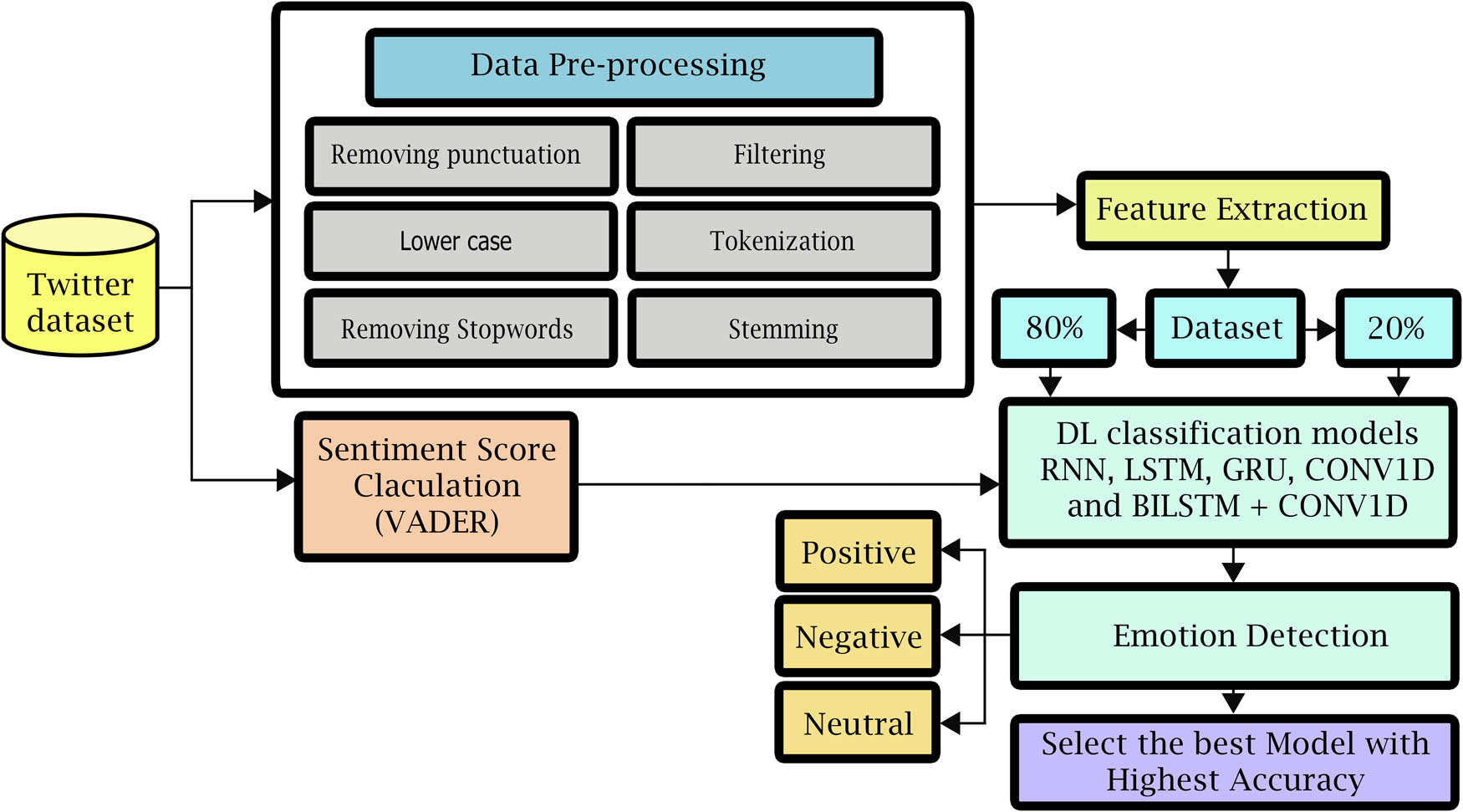
The proposed model for SA classification.

This model is distinguished by many advantages, as it relied on the LSTM method, which is characterized by its great ability to store data for a long time, which allowed the model to have a great ability to learn, including predicting effectively, which resulted in great accuracy in predicting the price of the cryptocurrency.

Table 1 presents an overview of each study’s literature evaluation, methodologies employed, and limitations. The findings indicate that deficiencies such as inaccuracies, reliance on rudimentary techniques, or limited sample sizes are common constraints encountered in the research. In the course of our study, we employed a variety of methodologies, including RNNs, LSTM networks, GRUs, CONV1D, Bi-LSTM + CONV1D, and several datasets of substantial magnitude sourced from the Kaggle platform. To extract features, we employed the Fasttext technique. The utilization of these various strategies contributed to the enhancement of accuracy.

5 Proposed model testing

This research aims to conduct experiments and evaluations on five DL models, namely RNN, LSTM, GRU, Bi-LSTM + CONV1D, and CONV1D. These experiments aim to assess their effectiveness in classifying the sentiment of BTC-related tweets.

5.1 Dataset

We downloaded BTC tweets from the Kaggle website, the dataset is available at Kaggle (https://www.kaggle.com/datasets/kaushiksuresh147/bitcoin-tweets), from February 10, 2021, to January 28, 2022. More than 1.5 million tweets were collected and tested using the suggested models to create the dataset. The research concentrated on SA of tweets to determine precisely and accurately how people felt about BTC. The dataset has a diverse range of columns, including user name, user location, a user created, and other information, as well as the tweet and user ratings, such as how many people marked the tweet as a favorite and the total number of user followers. Among these, the research particularly focuses on tweet text. The dataset was not labeled as positive, negative, or neutral, so this research used the VADER classifier to calculate polarity classification into positive, negative, or neutral.

5.2 Data preprocessing

The preliminary stage of the experiment is data preprocessing, which converts the raw data into an easily readable format to enhance the effectiveness and accuracy of the analysis; preprocessing is regarded as a vital step that must be completed before data are fed to the DL models, especially when the dataset being studied has a textual nature. There were several steps taken during the processing. Figure 2 shows tweets after preprocessing.

Figure 2

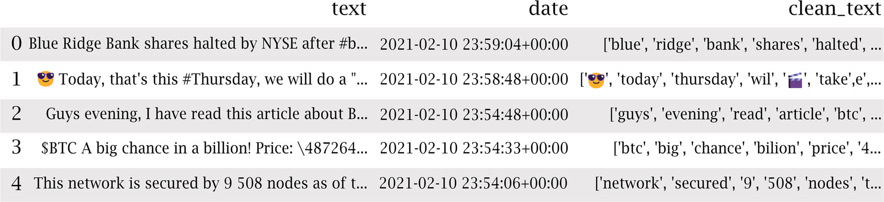
Tweets after preprocessing.

Removing punctuation: This eliminates punctuation, including commas, full stops, and exclamation points.
Convert to lower case: The tweets’ text has been lowercase. The analysis is case-sensitive; thus, this is a crucial step. For example, consider “HAPPY” and “happy” two different words.
Filtering: Remove all URL links, e.g., http://youtube.com, and delete tags from other usernames, which frequently start with an @ symbol.
Tokenization: Splitting of text into words and symbols.
Removing stop words: Deleting the stop words from the tweet text that are worthless in terms of SA, such as a, an, the, and all prepositions.
Stemming: Stemming is stripping words of their affixes and returning them to their original forms. Example: increases, increases, and increased are variations of increase.

5.3 Sentiment score calculation (VADER)

VADER is a dictionary- and rule-based open-source Python library for SA [31]. This library does not require text data for training and is appropriate for various texts, including social media. VADER calculates the input statement’s positive, negative, and neutral scores and offers a compound score, which is a numeric number between −1 and +1. Generally, a compound score between −1 and −0.05 is considered negative, one between 0.05 and 1 is regarded as positive, and the other values are considered neutral [8], as shown in Figure 3.

Figure 3

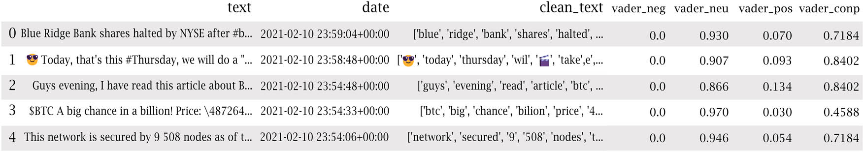
VADER sentiment score calculation.

5.4 Feature extraction

Identifying the word embedding method to transform the text into numerical representations is the first of the two key phases discussed in this section; in our case, it is FastText vector embedding. The second involves feeding the numerical representations of the text to the DL models for classification. Researchers from Facebook proposed FastText embedding in 2016 as an improvement to Word2Vec, an unsupervised learning algorithm to produce word vector representations, as explained in Section 3.3. This approach yields a matrix representing the dataset’s text as vectors. In order to create classification models, the results were obtained as vectors, which could be fed to the five DL algorithms.

5.5 DL models for sentiment classification

In this section, we present five DL classifiers as part of our proposal as follows: (1) RNN, (2) LSTM, (3) GRU, (4) Bi-LSTM + CONV1D, and (5) CONV1D. The architectural details of these models are presented in Tables 2–6.

Table 2

RNN model

Layer (type)	Output shape	Param #
embedding (Embedding)	(None, 50, 300)	30,000,000
simple_rnn (SimpleRNN)	(None, 50, 300)	180,300
simple_rnn (SimpleRNN)	(None, 64)	23,360
dense (Dense)	(None, 32)	2,080
dense_1 (Dense)	(None, 3)	99

Total params: 30,205,839. Trainable params: 205,839. Non-trainable params: 30,000,000.

Table 3

LSTM model

Layer (type)	Output shape	Param #
Embedding_2 (Embedding)	(None, 50, 300)	3,000,0000
lstm_2 (LSTM)	(None, 50, 300)	721,200
lstm_3 (LSTM)	(None, 100)	160,400
dense_4 (Dense)	(None, 32)	3,232
dense_5 (Dense)	(None, 3)	99

Total params: 30,884,931. Trainable params: 884,931. Non-trainable params: 30,000,000.

Table 4

GRU model

Layer (type)	Output shape	Param #
embedding_1 (Embedding)	(None, 50, 300)	3,000,0000
gru (GRU)	(None, 50, 200)	301,200
gru_1 (GRU)	(None, 100)	90,600
dense_2 (Dense)	(None, 32)	3,232
dense_3 (Dense)	(None, 3)	99

Total params: 30,395,131. Trainable params: 395,131. Non-trainable params: 30,000,000.

Table 5

Bi-LSTM + CONV1D model

Layer (type)	Output shape	Param #
embedding (Embedding)	(None, 50, 300)	3,000,0000
conv1d (CONV1D)	(None, 50, 32)	9,632
max_pooling1d(Max_pooling1D)	(None, 25, 32)	0
bidirectional (Bidirectional)	(None, 200)	106,400
dropout (Dropout)	(None, 200)	0
dense (Dense)	(None, 32)	6,432
dense_1 (Dense)	(None, 3)	99

Total params: 30,122,563. Trainable params: 122,563. Non-trainable params: 30,000,000.

Table 6

CONV1D model

Layer (type)	Output shape	Param #
embedding (Embedding)	(None, 50, 300)	30,000,000
conv1d (CONV1D)	(None, 50, 64)	134,464
max_pooling1d (Max_pooling1D)	(None, 25, 64)	0
conv1d (CONV1D)	(None, 25, 64)	28,736
global_max_pooling1d	(None, 64)	0
dropout (Dropout)	(None, 64)	0
dense (Dense)	(None, 32)	2,080
dense_1 (Dense)	(None, 3)	99

Total params: 30,165,379. Trainable params: 165,379. Non-trainable params: 30,000,000.

5.5.1 RNN model

When learning the embedding for each word in the training datasets, the “function embedding” layer is initially configured with random weights. The maximum length is 50, and the maximum output dimensions are 300. The matrix of the results is 50 × 300. The initial layer of the model is a simple RNN, which is responsible for accepting the vector generated by the process of word embedding. The model has a single RNN layer comprising 300 filters. These filters acquire and process data before forwarding it to the subsequent layer. The findings are presented in a matrix of 50 rows and 300 columns. The subsequent layer comprises a basic RNN that produces a matrix of dimensions 1 × 64. The classifier subsequently utilizes this matrix. Subsequently, the final phase within the model encompasses two fully connected layers. The initial layer employs the rectified linear unit (ReLU) as the chosen activation function (AF), comprising 32 nodes. The subsequent layer employs Softmax as the designated AF, containing three nodes. This configuration facilitates generating a multiclass categorical probability distribution, effectively reducing the vector to three elements. These elements correspond to the predicted output categories of “positive,” “negative,” or “neutral.” The Adam optimizer was employed to compute the learning rate in the present model.

5.5.2 LSTM model

The second DL classifier preprocessing is done on the input data to restructure it for the embedding matrix. The maximum length is 50, and the output dimensions are 300. The matrix of the results is 50 × 300. LSTM is the model’s first layer and gets the vector created by word embedding. The model has a single LSTM layer with 300 filters responsible for capturing and manipulating data before transmitting it to the subsequent layer. The results are presented in a matrix of 50 rows and 300 columns. The subsequent layer consists of an additional LSTM unit responsible for producing a matrix of dimensions 1 × 100. The classifier then uses this matrix. The model classifier is composed of two fully connected layers. The first layer employs the ReLU activation function with 32 nodes. The final layer utilizes the Softmax activation function with three nodes. The Adam optimization approach is used for the model.

5.5.3 GRU model

In the third DL classifier, the output from the embedding layer’s maximum length is 50, and the output dimensions are 300. The matrix of the results is 50 × 300. The first layer of the model is GRU, which receives the vector generated by word embedding. The model architecture includes a single GRU layer with 200 filters, responsible for capturing and processing input before forwarding it to subsequent layers. The results are shown in a matrix with dimensions of 50 rows and 200 columns. The subsequent layer consists of an additional GRU, responsible for producing a matrix of dimensions 1 × 100. The classifier then uses this matrix. The model classifier is composed of two fully connected layers. The first layer comprises 32 nodes and utilizes the ReLU activation function. The final layer, on the other hand, consists of three nodes and employs the Softmax activation function. The Adam optimizer approach is used in this model.

5.5.4 Bi-LSTM + Conv1D model

In the fourth DL classifier, the output from the embedding layer’s maximum length is 50, and the output dimensions are 300. The matrix of the results is 50 × 300. CONV1D serves as the model’s first layer and gets the vector created by word embedding. The model has a single CONV1D layer, including 32 filters responsible for data acquisition, processing, and subsequent propagation to the subsequent layer. The findings are presented in a matrix of 50 rows and 32 columns. A maximum-pooling layer is a common practice after a CNN layer. This is done to reduce the complexity of the output and mitigate the risk of overfitting the input. Consequently, the resulting matrix for this layer has dimensions of 25 × 32. The subsequent layer consists of a bidirectional LSTM model, which produces a matrix of dimensions 1 × 200. The classifier then uses this matrix. The use of a dropout layer in DL serves as a regularization technique to mitigate the issue of overfitting. Its primary function is to enforce independence among the units by preventing codependency. The model classifier is composed of two fully connected layers. The first layer comprises 32 nodes and utilizes the ReLU activation function. The final layer, on the other hand, consists of three nodes and employs the Softmax activation function. The Adam optimizer approach is used for the model.

5.5.5 CONV1D model

In the fifth DL classifier, the output from the embedding layer has a maximum length of 50, and the output dimensions are 300. The matrix of the results is 50 × 300. CONV1D serves as the model’s first layer and gets the vector created by word embedding. The model has a single CONV1D layer, including 64 filters responsible for data acquisition, processing, and subsequent transmission to the subsequent layer. The findings are presented in a matrix of 50 rows and 64 columns. Applying a maximum pooling layer follows a CNN layer to enhance the output’s simplicity and mitigate overfitting.

Consequently, the resulting matrix dimensions for this layer are 25 × 64. The second CNN is a CONV1D that produces a matrix of size 25 × 64, which is then used by the classifier. The Max Pooling1D layer reduces the dimensionality of the input representation by selecting the maximum value from each time dimension. This layer replaces flattening and occasionally even dense layers in classifiers and lowers the dimensionality of the feature maps produced by some convolutional layers. The dropout layer prevents overfitting problems. Next, the model classifier comprises 2 fully connected layers, the first using ReLU with 32 nodes, the last using Softmax with 3 nodes, and the Adam optimizer method.

6 Experimental results and discussion

This section provides a discussion of the findings obtained from the experiment.

6.1 Model training

In the first phase, we divided the dataset into two groups, 80% for training and 20% for testing, then trained using DL models to identify the best DL model. As described in Section 6.3, four evaluation measures were used to analyze and compare the DL classifiers: accuracy, precision, recall, and F1 score.

6.2 Epochs

The term “epoch” refers to the number of iterations performed on the training set. The generalization ability of the model demonstrates improvement with an increase in epochs. Nevertheless, when the number of epochs is very large, it might lead to the occurrence of overfitting, hence reducing the model’s ability to generalize [49]. Hence, selecting the optimal number of epochs is of utmost importance. In the present study, a total of 10 epochs were used.

Tables 7–11 show each epoch (loss, val_loss, accuracy, and val_accuracy) on the various DL models. As shown in Figures 4–8, the loss of the model reduces with each epoch during both the training and testing phases, suggesting that the model is performing optimally. The model’s accuracy for the training and testing phases is shown in Figures 9–13.

Table 7

Loss, Val loss, accuracy, Val accuracy of CONV1D model

Epoch	Loss	Val_Loss	Accuracy	Val_Accuracy
1/10	0.1748	0.1427	0.9307	0.9414
2/10	0.1316	0.1267	0.9464	0.9482
3/10	0.1176	0.1245	0.9524	0.9493
4/10	0.1090	0.1199	0.9564	0.9511
5/10	0.1030	0.1208	0.9591	0.9525

Table 8

Loss, Val loss, accuracy, Val accuracy OF LSTM model

Epoch	Loss	Val_Loss	Accuracy	Val_Accuracy
1/10	0.2274	0.1679	0.9127	0.9299
2/10	0.1622	0.1345	0.9336	0.9458
3/10	0.1390	0.1187	0.9423	0.9505
4/10	0.1265	0.1103	0.9475	0.9540
5/10	0.1188	0.1050	0.9507	0.9562

Table 9

Loss, Val loss, accuracy, Val accuracy of RNN model

Epoch	Loss	Val_Loss	Accuracy	Val_Accuracy
1/10	0.4037	0.4055	0.8697	0.8700
2/10	0.4045	0.4036	0.8700	0.8700
3/10	0.4046	0.4037	0.8700	0.8700
4/10	0.4045	0.4031	0.8700	0.8700
5/10	0.4041	0.4032	0.8700	0.8700

Table 10

Loss, Val loss, accuracy, Val accuracy OF GRU model

Epoch	Loss	Val_Loss	Accuracy	Val_Accuracy
1/10	0.1695	0.1365	0.9315	0.9431
2/10	0.1174	0.1123	0.9510	0.9533
3/10	0.1041	0.1069	0.9570	0.9565
4/10	0.0960	0.1041	0.9607	0.9570
5/10	0.0899	0.1044	0.9636	0.9582

Table 11

Loss, Val loss, accuracy, Val accuracy OF Bi-LSTM + CONV1D model

Epoch	Loss	Val_Loss	Accuracy	Val_Accuracy
1/10	0.1637	0.1311	0.9343	0.9447
2/10	0.1276	0.1235	0.9460	0.9489
3/10	0.1199	0.1161	0.9494	0.9509
4/10	0.1153	0.1124	0.9514	0.9531
5/10	0.1118	0.1099	0.9531	0.9534

Figure 4

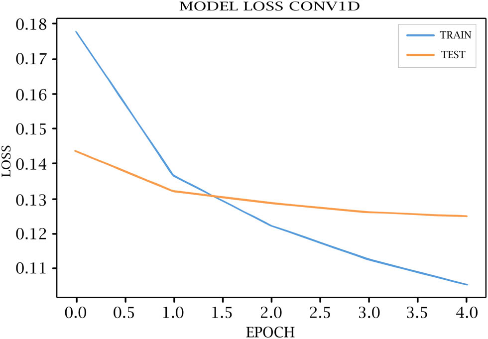
COV1D model loss for training and testing.

Figure 5

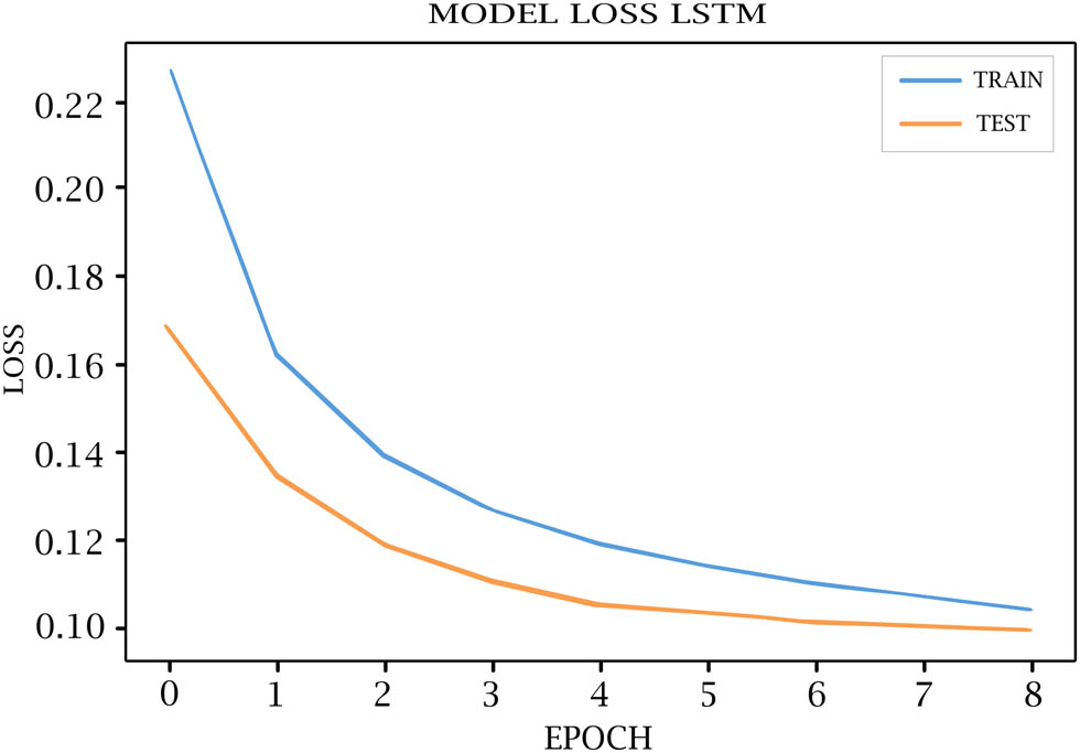
LSTM model loss for training and testing.

Figure 6

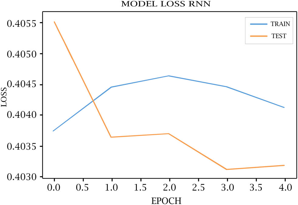
RNN model loss for training and testing.

Figure 7

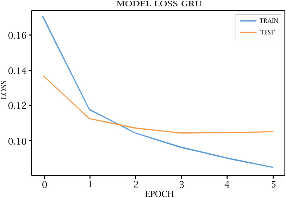
GRU model loss for training and testing.

Figure 8

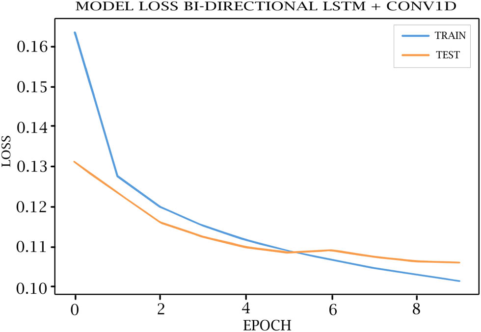
Bi-LSTM + CONV1D model loss for training and testing.

Figure 9

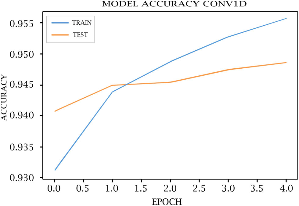
Cov1D model accuracy for training and testing.

Figure 10

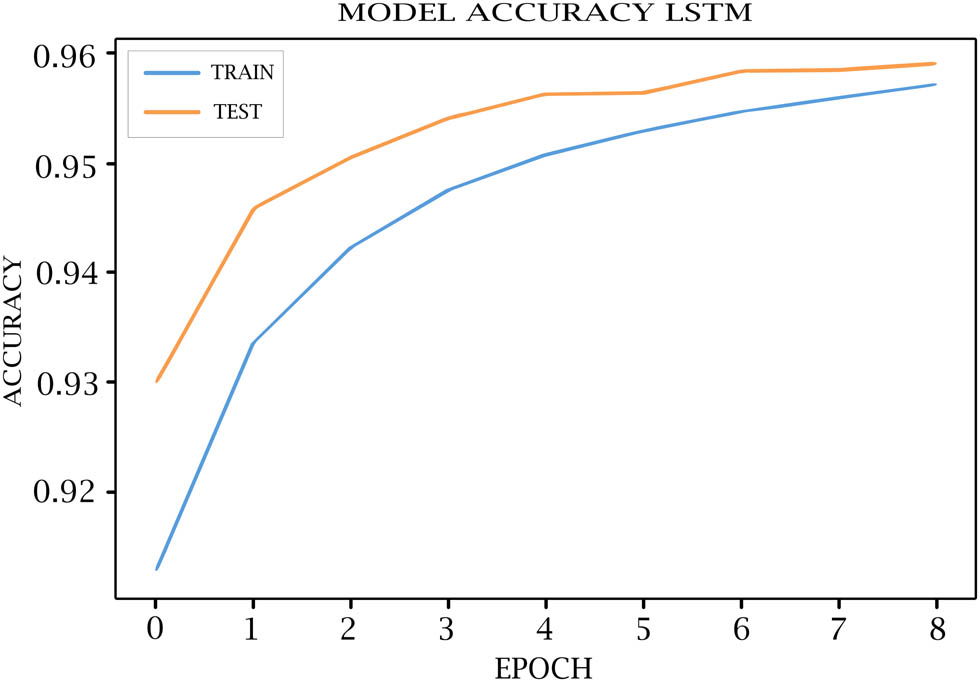
LSTM model accuracy for training and testing.

Figure 11

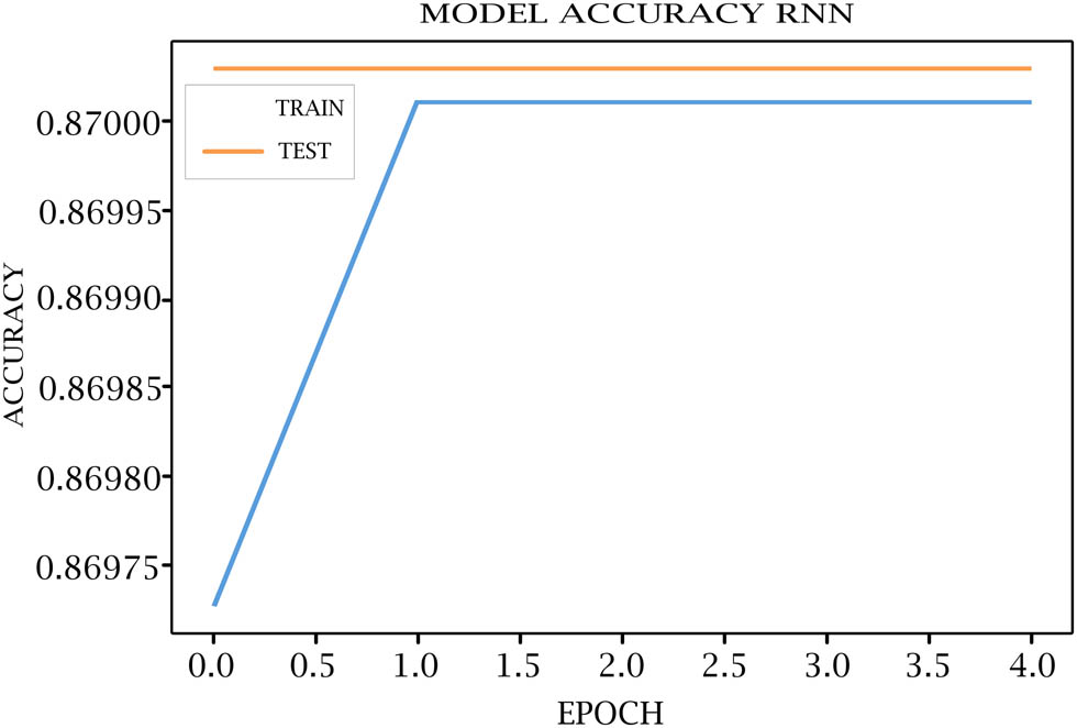
RNN model accuracy for training and testing.

Figure 12

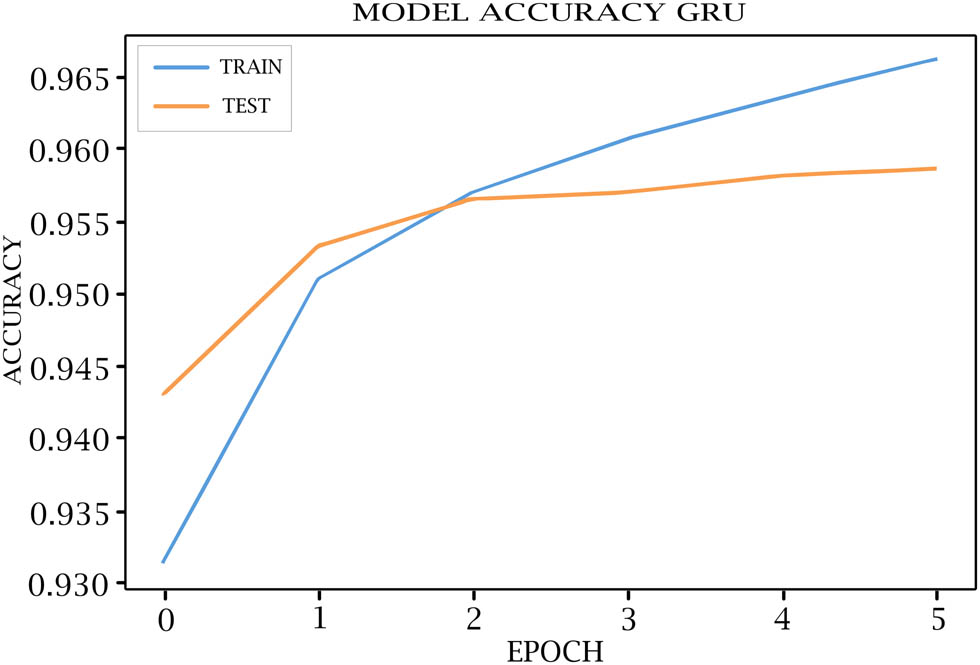
GRU model accuracy for training and testing.

Figure 13

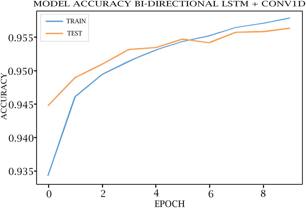
Bi-LSTM + CONV1D model accuracy for training and testing.

6.3 Evaluation metrics

We have evaluated the performance of the DL models with (precision, recall, F1 score, and accuracy).

Precision (P): It reflects the proportion of tuples with positive labels that are genuinely positive and is calculated by the following equation:

(1) Precision = TP TP + FP .

Recall (R): It indicates the proportion of successfully identified true positive tuples and is calculated by the following equation:

(2) Recall = TP TP + FN .

F 1 score: This is the weighted average of P and R and is calculated by the following equation:

(3) F 1 score = 2 × P × R P + R .

Accuracy: It represents the overall accuracy of the model and is calculated by and is:

(4) Accuracy = TP + TN TP + TN + FP + FN .

True positive (TP): Both real and expected values are true.

True negative (TN): Both real and expected values are false.

False positive (FP): When a real value is false, and the expected value is true.

False negative (FN): When a real value is true, and the expected value is false.

6.4 Confusion matrix

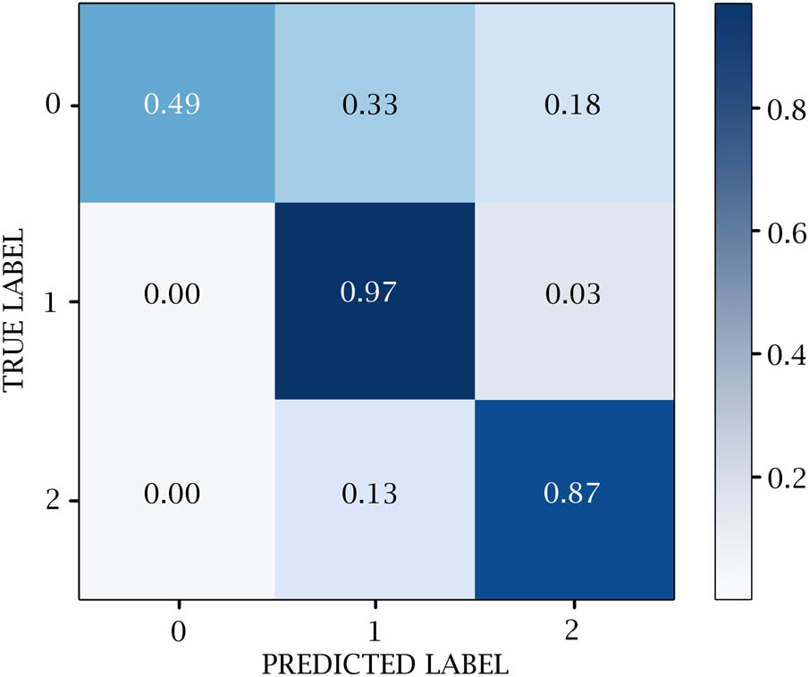
A confusion matrix is used to measure the efficacy of DL classifiers. TP, TN, FP, and FN values are generated over the test data. 0 represents the negative values, 1 represents the positive values, and 2 represents the neutral values. Figures 14–18 show the confusion matrix in DL models. Table 12 and Figure 19 show the negative, positive, and neutral sentiment counts for BTC tweets.

Figure 14

CONV1D confusion matrix.

Figure 15

LSTM confusion matrix.

Figure 16

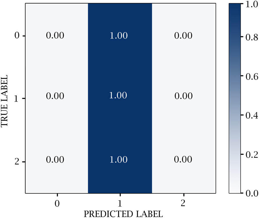
RNN confusion matrix.

Figure 17

GRU confusion matrix.

Figure 18

Bi-LSTM + CONV1D confusion matrix.

Table 12

Count of negative, positive, and neutral sentiments

Model name	Negative count	Positive count	Neutral count
CONV1D	641	171,580	17,810
LSTM	1,082	202,714	26,368
RNN	0	208,806	0
GRU	1,058	202,840	25,985
Bi-LSTM + CONV1D	949	202,458	26,114

Figure 19

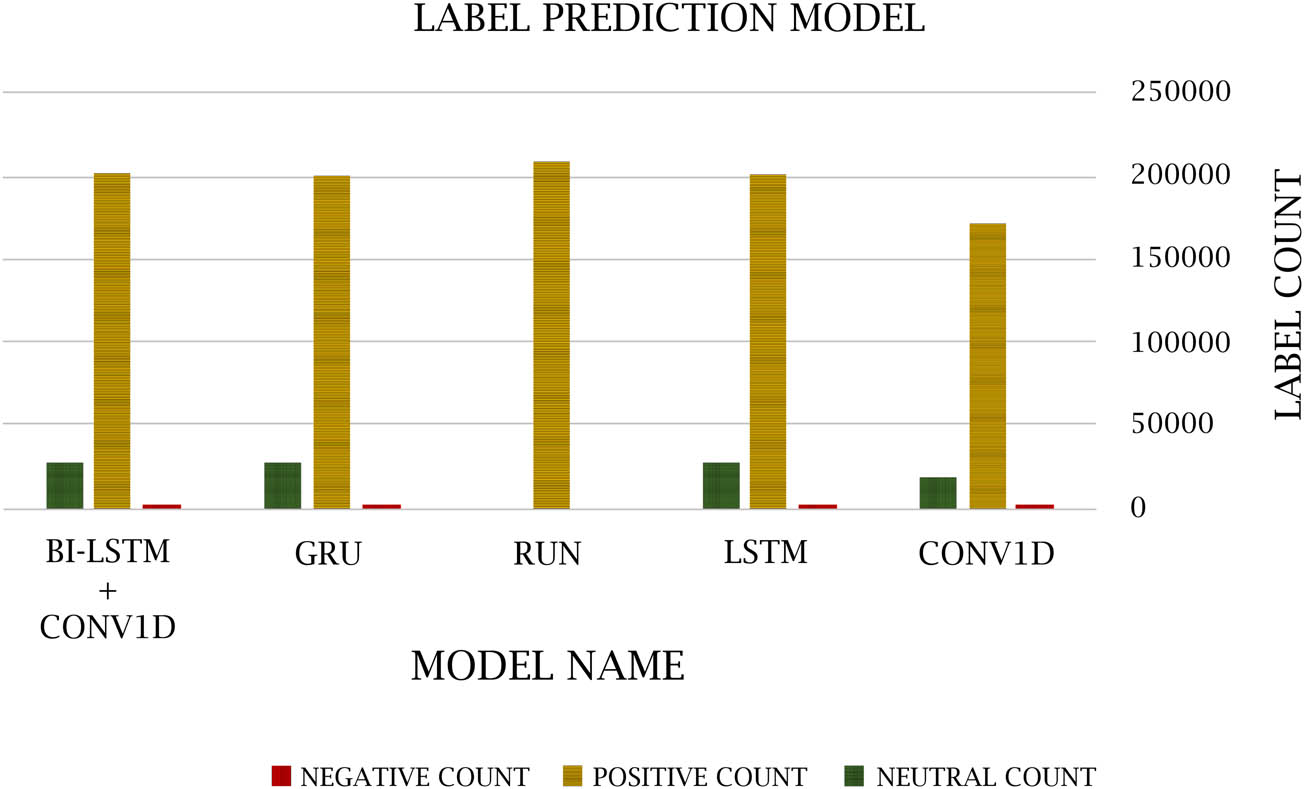
Negative, positive, and neutral sentiments.

6.5 DL Classification model Outcomes

This section discussed the results of classification models obtained using a DL classifier. The performance of classification outcomes in terms of accuracy, recall, and F1-score is shown in Tables 13–17. Figure 20 shows the DL models’ accuracy.

Table 13

Evaluation results for CONV1D model

Class	Precision	Recall	F1-Score	Accuracy
0	0.93	0.49	0.64	0.95
1	0.98	0.97	0.97
2	0.80	0.87	0.83
Macro avg	0.90	0.78	0.82
Weighted avg	0.96	0.95	0.95

Table 14

Evaluation results for LSTM model

Class	Precision	Recall	F1-Score	Accuracy
0	0.86	0.58	0.69	0.96
1	0.98	0.97	0.98
2	0.90	0.90	0.85
Macro avg	0.88	0.82	0.84
Weighted avg	0.96	0.96	0.96

Table 15

Evaluation results for RNN model

Class	Precision	Recall	F1-score	Accuracy
0	0.00	0.00	0.00	0.87
1	0.87	1.00	0.93
2	0.00	0.00	0.00
Macro avg	0.29	0.33	0.31
Weighted avg	0.76	0.87	0.81

Table 16

Evaluation results for GRU model

Class	Precision	Recall	F1-score	Accuracy
0	0.89	0.55	0.68	0.96
1	0.98	0.97	0.98
2	0.82	0.88	0.85
Macro avg	0.90	0.80	0.83
Weighted avg	0.96	0.96	0.96

Table 17

Evaluation results for Bi-LSTM + CONV1D model

Class	Precision	Recall	F1-score	Accuracy
0	0.92	0.51	0.65	0.96
1	0.98	0.97	0.98
2	0.89	0.89	0.84
Macro avg	0.90	0.79	0.82
Weighted avg	0.96	0.96	0.96

Figure 20

DL model accuracy.

Twitter is a significant, well-liked microblog where users express their perspectives on current events. SA has recently focused mostly on assessing these viewpoints. Researchers have found recording, collecting, and analyzing people’s feelings difficult to overcome these issues. This study suggests DL models for the SA of tweets. In order to improve sentiment classification’s performance and accuracy, we used a DL technique in this article together with CONV1D, LSTM, RNN, GRU, and Bi-LSTM + CONV1D classifier models.

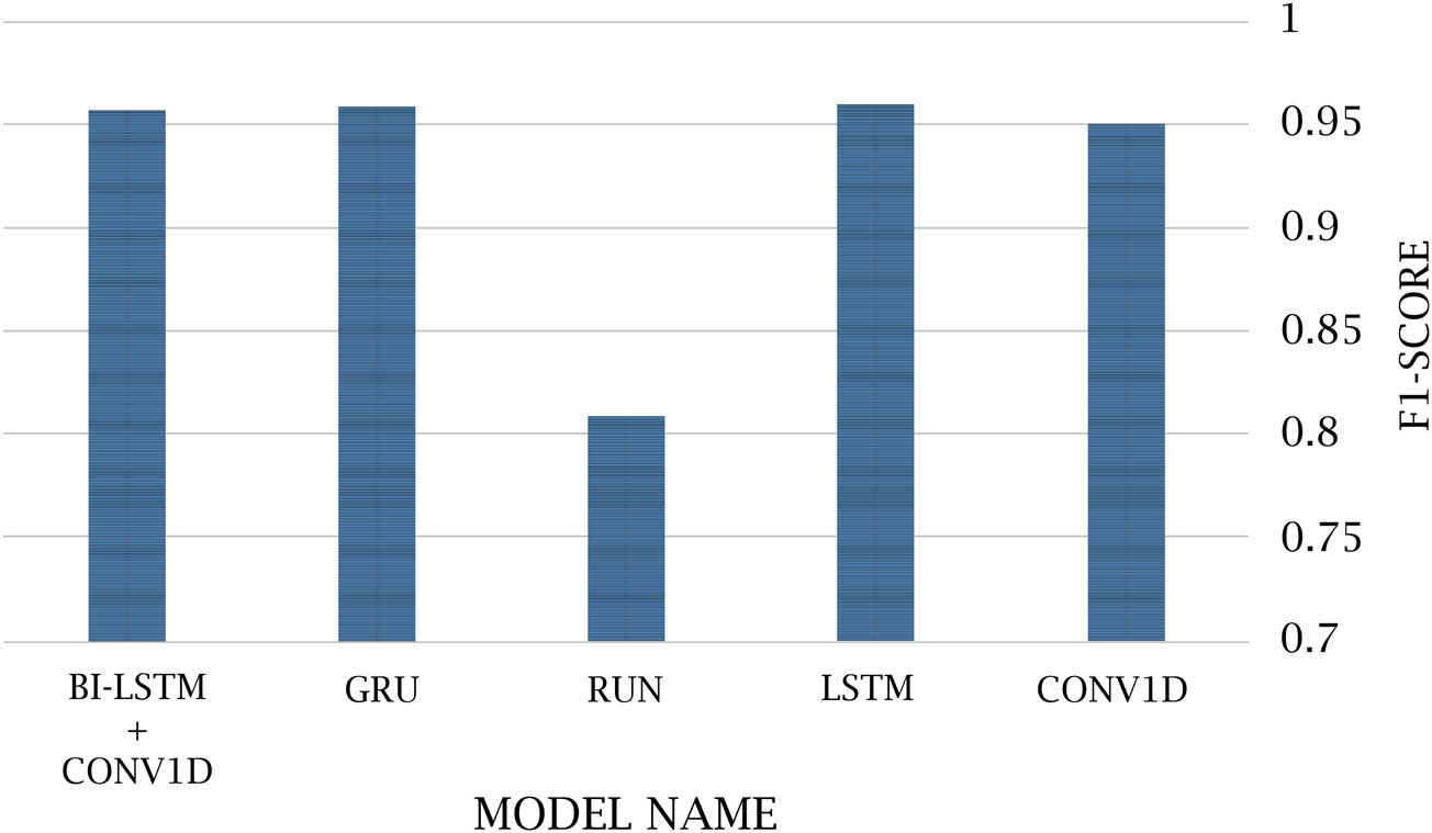
Additionally, the research emphasizes how crucial feature extraction and preprocessing are to the sentiment classification approach. The tweets in the text were divided into a training dataset and a testing dataset for the research, which was based on BTC tweets. For this comparison, we used CONV1D, LSTM, RNN, GRU, and Bi-LSTM + CONV1D. In comparison, the suggested DL classifiers have an accuracy rate of 95.01, 95.95, 80.59, 95.82, and 95.67%, respectively. Table 18 shows the accuracy of DL model classifiers’ results summaries.

Table 18

Accuracy of DL model result summary

Model name	F1-score
CONV1D	0.95010
LSTM	0.95950
RNN	0.80950
GRU	0.95822
Bi-LSTM + CONV1D	0.95672

7 Conclusions and future work

Table 1 of the literature evaluation provides a comprehensive description of the techniques used in each research and an overview of the limitations associated with these methodologies. During our investigation, we used analogous and disparate models in conjunction with a considerable-sized dataset. The utilization of models collectively contributed to the enhancement of accuracy.

DL classification models and a FastText-based approach were used to determine the sentiment or polarity of the dataset. Table 18 shows different DL models’ overall accuracy, precision, recall, and F1-score. The performance accuracy of the CONV1D, LSTM, RNN, GRU, and Bi-LSTM + CONV1D models was 95.01, 95.95, 80.59, 95.82, and 95.67%, respectively. The LSTM, GRU, and Bi-LSTM + CONV1D models produce more precise results than other DL models, so as shown in Table 18, the LSTM model gives the best result. This study also used a BTC Twitter dataset with textual information in English.

In the future, we look forward to applying other languages to the proposed model that has been built. We also look forward to using other DL algorithms or hybrid DL models to improve emotion classification accuracy. The epoch size could also be raised to obtain a higher accuracy percentage. We also look forward in the future to presenting a research article that examines the measurement of the correlation between tweets and the subsequent influence on cryptocurrency prices. Finally, we anticipate the utilization of these algorithms across diverse domains to ascertain their efficacy and precision.

8 Research limitations

The following points may delineate the limits of the research:

In this research, an SA was conducted only on the cryptocurrency BTC. There is potential for the expansion of this research to include more digital currencies.
The research was carried out using the BTC comment corpus, which only comprises textual data in the English language. The authors express their anticipation for the future application of the suggested approach to more languages in forthcoming research.
This research focused on classifying comments about the BTC currency and obtaining the highest possible accuracy for analyzing the sentiment of the tweets, and not calculating the correlation coefficient between the tweets and the price of the currency and its effect, whether rising or falling.

Acknowledgments

The authors thank the editor and reviewers for their valuable comments and suggestions that improved the manuscript.

Funding information: The authors state no funding involved.
Author contributions: Michael Nair: The literature review, the experiment part, producing the result, and Writing parts of the paper; Laila A. Abd-Elmegid: Drawing the paper structure and methodology, introducing the problem, and reviewing the results; Mohamed I. Marie: Reviewing the whole paper, reviewing the results, and analyzing the results.
Conflict of interest: The authors declare that there is no conflict of interest.
Data availability statement: This research uses an online data set that is appropriately cited within the article and can be found online.

References

[1] Fakharchian S. Designing forecasting assistant of the Bitcoin price based on deep learning using the market sentiment analysis and multiple feature extraction. Soft Comput. 2023;27(24):18803–27.10.1007/s00500-023-09028-5Search in Google Scholar

[2] Parekh R, Patel NP, Thakkar N., Gupta R, Tanwar S, Sharma G, et al. DL-GuesS: Deep learning and sentiment analysis-based cryptocurrency price prediction. IEEE Access. 2022;10:35398–35409. 10.1109/ACCESS.2022.3163305.Search in Google Scholar

[3] Şaşmaz E, Tek FB. Tweet sentiment analysis for cryptocurrencies. Proceedings - 6th International Conference on Computer Science and Engineering, UBMK 2021; 2021. p. 613–8. 10.1109/UBMK52708.2021.9558914.Search in Google Scholar

[4] Sattarov O, Jeon HS, Oh R, Lee JD. Forecasting Bitcoin price fluctuation by twitter sentiment analysis. 2020 International Conference on Information Science and Communications Technologies, ICISCT 2020; Nov. 2020. 10.1109/ICISCT50599.2020.9351527.Search in Google Scholar

[5] Kaur G, Malik K. A sentiment analysis of airline system using machine learning algorithms. Int J Adv Res Eng. 2021;12(1):731–42. 10.34218/IJARET.12.1.2021.066.Search in Google Scholar

[6] Mahto D, Yadav SC, Lalotra GS. Sentiment prediction of textual data using hybrid convbidirectional-LSTM model. Mobile Information Systems. 2022;2022:1068554. 10.1155/2022/1068554.Search in Google Scholar

[7] Kraaijeveld O, de Smedt J. The predictive power of public Twitter sentiment for forecasting cryptocurrency prices. J Int Financ Mark Inst Money. Mar. 2020;65:101188. 10.1016/J.INTFIN.2020.101188.Search in Google Scholar

[8] Ye Z, Wu Y, Chen H, Pan Y, Jiang Q. A stacking ensemble deep learning model for Bitcoin price prediction using twitter comments on Bitcoin. Mathematics. Apr. 2022;10(8):1307. 10.3390/MATH10081307.Search in Google Scholar

[9] Singh C, Imam T, Wibowo S, Grandhi S. A deep learning approach for sentiment analysis of COVID-19 reviews. Appl Sci. Apr. 2022;12(8):3709. 10.3390/APP12083709.Search in Google Scholar

[10] Mardjo A, Choksuchat C. HyVADRF: Hybrid VADER-random forest and GWO for Bitcoin tweet sentiment analysis. IEEE Access. 2022;10:101889–97. 10.1109/ACCESS.2022.3209662.Search in Google Scholar

[11] Kilimci ZH. Sentiment analysis based direction prediction in Bitcoin using deep learning algorithms and word embedding models. Int J Intell Syst Appl Eng. Jun. 2020;8(2):60–5. 10.18201/ijisae.2020261585.Search in Google Scholar

[12] Raju SM, Tarif AM. Real-time prediction of Bitcoin price using machine learning techniques and public sentiment analysis. ArXiv. Jun. 2020. 10.48550/arXiv.2006.14473.Search in Google Scholar

[13] Umer M, Ashraf I, Mehmood A, Kumari S, Ullah S, Sang Choi G. Sentiment analysis of tweets using a unified convolutional neural network-long short-term memory network model. Comput Intell. Feb. 2021;37(1):409–34. 10.1111/COIN.12415.Search in Google Scholar

[14] Yao G. Deep learning-based text sentiment analysis in Chinese international promotion. Secur Commun Netw. 2022;2022:1–10. 10.1155/2022/7319656.Search in Google Scholar

[15] Hussein M, Özyurt F. A new technique for sentiment analysis system based on deep learning using chi-square feature selection methods. Balk J Electr Computer Eng. Oct. 2021;9(4):320–6. 10.17694/bajece.887339.Search in Google Scholar

[16] Passalis N, Avramelou L, Seficha S, Tsantekidis A, Doropoulos S, Makris G, et al. Multisource financial sentiment analysis for detecting Bitcoin price change indications using deep learning. Neural Comput Appl. Nov. 2022;34(22):19441–52. 10.1007/S00521-022-07509-6/TABLES/5.Search in Google Scholar

[17] Saha J, Patel S, Xing F, Cambria E. Does social media sentiment predict Bitcoin trading volume? ICIS 2022 Proceedings; Dec. 2022. Accessed: Feb. 20, 2023. [Online]. https://aisel.aisnet.org/icis2022/blockchain/blockchain/3.Search in Google Scholar

[18] Aslam N, Rustam F, Lee E, Washington PB, Ashraf I. Sentiment analysis and emotion detection on cryptocurrency related tweets using ensemble LSTM-GRU model. IEEE Access. 2022;10:39313–24. 10.1109/ACCESS.2022.3165621.Search in Google Scholar

[19] Huang X, Zhang W, Tang X, Zhang M, Surbiryala J, Iosifidis V, et al. LSTM based sentiment analysis for cryptocurrency prediction. Lecture notes in computer science (including subseries Lecture Notes in Artificial Intelligence and Lecture Notes in Bioinformatics) LNCS. Vol. 12683; 2021. p. 617–21. 10.1007/978-3-030-73200-4_47/TABLES/2.Search in Google Scholar

[20] Jahjah FH, Rajab M. Impact of twitter sentiment related to Bitcoin on stock price returns. J Eng. Jun. 2020;26(6):60–71. 10.31026/J.ENG.2020.06.05.Search in Google Scholar

[21] Pant DR, Neupane P, Poudel A, Pokhrel AK, Lama BK. Recurrent neural network based Bitcoin price prediction by twitter sentiment analysis. Proceedings on 2018 IEEE 3rd International Conference on Computing, Communication and Security, ICCCS 2018; Dec. 2018. p. 128–32. 10.1109/CCCS.2018.8586824.Search in Google Scholar

[22] Onan A. GTR-GA: Harnessing the power of graph-based neural networks and genetic algorithms for text augmentation. Expert Syst Appl. 2023;232:120908. 10.1016/j.eswa.2023.120908.Search in Google Scholar

[23] Onan A. SRL-ACO: A text augmentation framework based on semantic role labeling and ant colony optimization. J King Saud Univ-Computer Inf Sci. 2023;35:101611. 10.1016/j.jksuci.2023.101611‏.Search in Google Scholar

[24] Onan A. Hierarchical graph-based text classification framework with contextual node embedding and BERT-based dynamic fusion. J King Saud Univ-Computer Inf Sci. 2023;35:101610. 10.1016/j.jksuci.2023.101610.Search in Google Scholar

[25] Onan A. Bidirectional convolutional recurrent neural network architecture with group-wise enhancement mechanism for text sentiment classification. J King Saud Univ-Computer Inf Sci. 2022;34(5):2098–117. 10.1016/j.jksuci.2022.02.025.Search in Google Scholar

[26] Onan A. Sentiment analysis on massive open online course evaluations: a text mining and deep learning approach. Computer Appl Eng Educ. 2021;29(3):572–89. 10.1002/cae.22253.Search in Google Scholar

[27] Onan A, Toçoğlu MA. A term weighted neural language model and stacked bidirectional LSTM based framework for sarcasm identification. IEEE Access. 2021;9:7701–22. 10.1109/ACCESS.2021.3049734.Search in Google Scholar

[28] Beigi G, Hu X, Maciejewski R, Liu H. An overview of sentiment analysis in social media and its applications in disaster relief. Stud Comput Intell. 2016;639:313–40. 10.1007/978-3-319-30319-2_13/TABLES/2.Search in Google Scholar

[29] Ruz GA, Henríquez PA, Mascareño A. Sentiment analysis of Twitter data during critical events through Bayesian networks classifiers. Future Gener Computer Syst. May 2020;106:92–104. 10.1016/J.FUTURE.2020.01.005.Search in Google Scholar

[30] Lazrig I, Humpherys SL. Using machine learning sentiment analysis to evaluate learning impact. Inf Syst Educ J. Feb. 2022;20(1):13–21. Accessed: Feb. 20, 2023. [Online]. https://isedj.org/;https://iscap.info.Search in Google Scholar

[31] Nawaz N, Deep learning-based sentiment analysis and topic modeling on tourism during COVID-19 pandemic. Dec. 27, 2021. Accessed: Feb. 20, 2023. [Online]. https://papers.ssrn.com/abstract=3994359.Search in Google Scholar

[32] Li Y, Yang T. Word embedding for understanding natural language: A survey. Stud Big Data. 2018;26:83–104. 10.1007/978-3-319-53817-4_4/FIGURES/8.Search in Google Scholar

[33] Mojumder P, Hasan M, Hossain MF, Hasan KMA. A study of fasttext word embedding effects in document classification in bangla language. Lecture Notes of the Institute for Computer Sciences, Social-Informatics and Telecommunications Engineering, LNICST. Vol. 325; 2020. p. 441–53. 10.1007/978-3-030-52856-0_35/TABLES/5.Search in Google Scholar

[34] Dang CN, Moreno-García MN, de La Prieta F. Hybrid deep learning models for sentiment analysis. Complexity. 2021;2021. 10.1155/2021/9986920.Search in Google Scholar

[35] Umer M, et al. Impact of convolutional neural network and FastText embedding on text classification. Multimed Tools Appl. Feb. 2023;82(4):5569–85. 10.1007/S11042-022-13459-X/FIGURES/3.Search in Google Scholar

[36] Karlemstrand R, Leckström E, Using twitter attribute information to predict stock prices. arXiv preprint. Stockholm. May 2021. 10.48550/arxiv.2105.01402.Search in Google Scholar

[37] Chandio BA, Imran AS, Bakhtyar M, Daudpota SM, Baber J. Attention-based RU-BiLSTM sentiment analysis model for Roman Urdu. Appl Sci. Apr. 2022;12(7):3641. 10.3390/APP12073641.Search in Google Scholar

[38] Irie K, Csordás R, Urgen Schmidhuber J. The dual form of neural networks revisited: Connecting test time predictions to training patterns via spotlights of attention. PMLR. Jun. 28, 2022;9639–59. Accessed: Feb. 20, 2023. [Online]. https://proceedings.mlr.press/v162/irie22a.html.Search in Google Scholar

[39] Rodrigues AP, Fernandes R, Shetty A, Lakshmanna K, Shafi RM. Real-time twitter spam detection and sentiment analysis using machine learning and deep learning techniques. Comput Intell Neurosci. 2022;2022:1–14. 10.1155/2022/5211949.Search in Google Scholar PubMed PubMed Central

[40] Bhowmik NR, Arifuzzaman M, Mondal MRH. Sentiment analysis on Bangla text using extended lexicon dictionary and deep learning algorithms. Array. Mar. 2022;13:100123. 10.1016/J.ARRAY.2021.100123.Search in Google Scholar

[41] Alam KN, Khan MS, Dhruba AR, Khan MM, Al-Amri JF, Masud M, et al. Deep learning-based sentiment analysis of COVID-19 vaccination responses from twitter data. ArXiv, p. arXiv: 2209.12604. Aug. 2022. 10.48550/ARXIV.2209.12604.Search in Google Scholar

[42] Liu D, Wei A. Regulated LSTM artificial neural networks for option risks. FinTech. Jun. 2022;1(2):180–90. 10.3390/FINTECH1020014.Search in Google Scholar

[43] Bilgili M, Arslan N, Sekertekin A, Yasar A. Application of long short-term memory (LSTM) neural network based on deeplearning for electricity energy consumption forecasting. Turkish J Electr Eng Computer Sci. Jan. 2022;30(1):140–57. 10.3906/elk-2011-14.Search in Google Scholar

[44] Wang C, Yan H, Huang W. AGA-GRU: An optimized GRU neural network model based on adaptive genetic algorithm. J Phys Conf Ser. Nov. 2020;1651(1):012146. 10.1088/1742-6596/1651/1/012146.Search in Google Scholar

[45] Zarzycki K, Ławryńczuk M. Advanced predictive control for GRU and LSTM networks. Inf Sci (N Y). Nov. 2022;616:229–54. 10.1016/J.INS.2022.10.078.Search in Google Scholar

[46] Elfaik H, Nfaoui EH. Deep bidirectional LSTM network learning-based sentiment analysis for Arabic text. J Intell Syst. Jan. 2021;30(1):395–412. 10.1515/JISYS-2020-0021/ASSET/GRAPHIC/J_JISYS-2020-0021_FIG_008.JPG.Search in Google Scholar

[47] Yousaf K, Nawaz T. A deep learning-based approach for inappropriate content detection and classification of youtube videos. IEEE Access. 2022;10:16283–98. 10.1109/ACCESS.2022.3147519.Search in Google Scholar

[48] Mahalakshmi P, Fatima NS. Ensembling of text and images using Deep Convolutional Neural Networks for Intelligent Information Retrieval. Wirel Pers Commun. Nov. 2022;127(1):235–53. 10.1007/S11277-021-08211-X/METRICS.Search in Google Scholar

[49] Xu G, Meng Y, Qiu X, Yu Z, Wu X. Sentiment analysis of comment texts based on BiLSTM, IEEE Access. 2019;7:51522–32. 10.1109/ACCESS.2019.2909919.Search in Google Scholar

Received: 2023-06-30

Revised: 2023-11-09

Accepted: 2023-12-14

Published Online: 2024-03-11

This work is licensed under the Creative Commons Attribution 4.0 International License.

Articles in the same Issue

https://doi.org/10.1515/jisys-2023-0085

Keywords for this article

cryptocurrency; deep learning; algorithms; sentiment analysis; natural language processing; preprocessing

Creative Commons

BY 4.0