Integration of numerical models to simulate 2D hydrodynamic/water quality model of contaminant concentration in Shatt Al-Arab River with WRDB calibration tools

Mohammed Jabbar Mawat; Ahmed Naseh Ahmed Hamdan

doi:10.1515/eng-2022-0416

Artikel Open Access

Integration of numerical models to simulate 2D hydrodynamic/water quality model of contaminant concentration in Shatt Al-Arab River with WRDB calibration tools

Mohammed Jabbar Mawat und Ahmed Naseh Ahmed Hamdan

Veröffentlicht/Copyright: 26. Juni 2023

Veröffentlicht von

Veröffentlichen auch Sie bei De Gruyter Brill

Manuskript einreichen Informationen für Autor*innen

Aus der Zeitschrift Open Engineering Band 13 Heft 1

Abstract

The hydrodynamic model is essential for building a water quality model for rivers, lakes, estuaries, and other water systems. Most model software, such as HEC-RAS, can perform a complex hydrodynamic surface water body and limitations to represent water quality for the corresponding area. In contrast, other models, like WASP, can simulate a wide range of contaminants in a multidimensional geometry of rivers, estuaries, lakes, and reservoirs. Still, it requires flow information from separate hydrodynamic models. This article aims to develop a comprehensive water quality model of the Shatt Al Arab River south of Iraq by linking HEC-RAS with WASP. A variety of software techniques has sequentially been used. This software includes GIS for DEM modification, HEC-RAS for the hydrodynamic model, Python code with PyCharm to run the external coupler, WASP software for advective and dispersive contaminant transport, and finally, WRDB software for full calibration process and results display. The results showed successful transportation of flow information had been achieved. Moreover, the article described an effective calibration process by plotting comparison graphs and statistical summaries to make the appropriate decision. Another goal of this work is to collect the equations and associated reaction rates of source/sink kinetic for eutrophication’s state variables.

Keywords: hydrodynamic modeling; water quality modeling; HEC-RAS; WASP; WRDB; external coupling; Shatt Al-Arab modeling

1 Introduction

The modeling of surface water is complex and developing [1]. Professionals disagree with the “optimal” way of modeling rivers, lakes, estuaries, and coastal waters [2]. Even after more than a century, the basic approach to surface water modeling has not altered because all models are built on three fundamental principles: mass, momentum, and energy conservation [3,4]. The most general classification of modules used in surface waters modeling is analytical or numerical models [1]: An analytical model has an exact mathematical solution to the governing equations that describe processes in a body of water. An analytical solution example for estimating the concentrations of dissolved oxygen (DO) along rivers is the Streeter–Phelps (1925) equation [5]. A numerical model is a discretized representation of a mathematical equation system that explains processes in a water body. The computing domain is discretized into cells, and the partial differential governing equations are approximated by a set of algebraic equations solved by the iteration or the matrix inversion method. In recent years, computer simulation techniques have gained popularity in scientific studies, particularly regarding studies of the aquatic environment. Many computer models have been created and are effectively used in many countries today [1]. Review research studies from the Web of Science focused on the fate and transport of water quality modules in waterbodies, such as EFDC, CE-QUAL-W2, WASP, Delft3D, AQUATOX, and MIKE, are listed in Table 1. The highest models utilized in uses and citations were EFDC and CE-QUAL-W2. The United States and China were the most frequent users of such models [6]. Fu et al. [7] searched the Scopus database for 50,530 publications on water quality models published between 1935 and 2018. 76% of the publications (38,542) were published between 2003 and 2018. Most of these articles were published by authors with locations in the United States, followed by China, the United Kingdom, Germany, Canada, and Australia.

Table 1

Research records about water quality modeling (2001–2022)

Model	EFDC	CE-QUAL-W2	WASP	Delft3D	AQUATOX	MIKE
Article/review	210	179	143	74	50	132

The following paragraphs will cover a variety of research that used standard computer models with their most prominent results.

Ramos-Ramírez et al. [8] undertook water quality simulations of the dispersion of Chrome III (Cr III) in the Bogotá River, Cundinamarca, Colombia. The WASP model was employed in the simulation’s construction to reflect the Cr III dispersion under the research circumstances. Using the most recent 1D, 2D, and 3D modeling software, Marvin and Wilson [9] described the thorough hydrodynamic modeling done for the estuary of Salmon River and its branches as a portion of an overall flood hazard analysis. Alam et al. [10] investigated the impacts of rising temperatures and solar radiation from climate change on the Sitalakhya River’s water quality using WASP. Chuersuwan et al. [11], with the help of WASP, aimed to empower local authorities on water quality management in the Lamtakhong river’s basin, Thailand. Yen et al. [12] investigated pollution sources and water quality comprehensively, followed by implementing the WASP model to develop water quality requirements in Carp Lake, Taiwan. In surface water quality modeling, the model coupling is a significant trend. The integrated modeling technique is more sophisticated and difficult to master than the conventional. The main obstacles to the coupling process are a lack of observed data, bathymetry information, model parameter estimates, and computational time [13]. WASP has been proved in the literature to be capable of simulating river transport. It has been integrated with several hydraulic tools, frequently for water quality modeling via external Linkage to hydraulic models for water flow information. The prominent instances are as follows.

Chueh et al. [14] simulated the copper concentration using SWAT and WASP in the Erren River. SWAT was used to compute non-point source (NPS) soil erosion, while WASP was used to simulate copper concentrations in both the aqueous and sediment phases. Zhu et al. [15] investigated a unidirectional link of the urban hydrological and hydraulic models CS-TARP, WASP, and EFDC that were used to simulate the influence of sewer overflows on nutrients in the Chicago River. Define et al. [16] combined the Regional Ocean Modeling System (ROMS) with WASP to conduct a thorough examination of water quality in Barnegat Bay, New Jersey. A WASP model integrated with the HEC-HMS model estimated mercury transport and fractionation in the Xiaxi River, China [17]. Yin and Seo [18] developed a three-dimensional model using an integrated hydrodynamic Environmental Fluid Dynamics Code (EFDC) and water quality model WASP for the Ara Canal in Korea that connects the Han River and the Yellow Sea. SWAT and WASP simulations of the watershed NPS load and internal flow in the Cedar Creek Reservoir, according to Ernst and Owens [19], had the greatest effect on chl a and TP. Wool et al. [20] employed WASP and hydrodynamics data from EFDC to estimate eutrophication, nutrient circulation, and DO kinetic in the Neuse River estuary, United States. Rodriguez and Peene [21] developed a two-dimensional hydrodynamic, transport, and water quality model in order to determine the allowable total maximum daily load (TMDL) for oxygen-demanding materials. The 2D vertically averaged hydrodynamic model (EFDC) was combined with WASP.

This article aims to develop a comprehensive water quality model of the Shatt Al-Arab River south of Iraq by linking HEC-RAS with WASP. Moreover, the article described an effective calibration process by plotting comparison graphs and statistical summaries to make the appropriate decision. Another goal of this work is to collect the equations and associated reaction rates of source/sink kinetic for eutrophication’s state variables.

2 Materials and methods

2.1 Description of the study area

The Tigris and Euphrates Rivers meet near Al- the Qurna district in southern Iraq to form the Shatt Al-Arab River [22] (Figure 1). The Shatt Al-Arab River is a 192-km-length tidal river that flows south-eastwards, passing through Basrah and then discharging into the Arabian Gulf [23]. The River’s width changes along its length, from 250 to 300 m near the Euphrates-Tigris confluence to 600 m around the town of Basrah and 2,000 m at the estuary [24]. For the last 95 km of its course, the River forms part of the border between Iraq and Iran [25]. In addition to transportation, the Shatt Al-Arab River has an important role in delivering water for domestic use, irrigation, and manufacturing [26]. Several water treatment plants along the River divert water for household use. Currently, contributions of River feeders have been decreased due to surrounding governments’ policies, which resulted in a significant increase in TDS values in the Shatt Al-Arab River due to the effect of the Arabian Gulf [27].

Figure 1

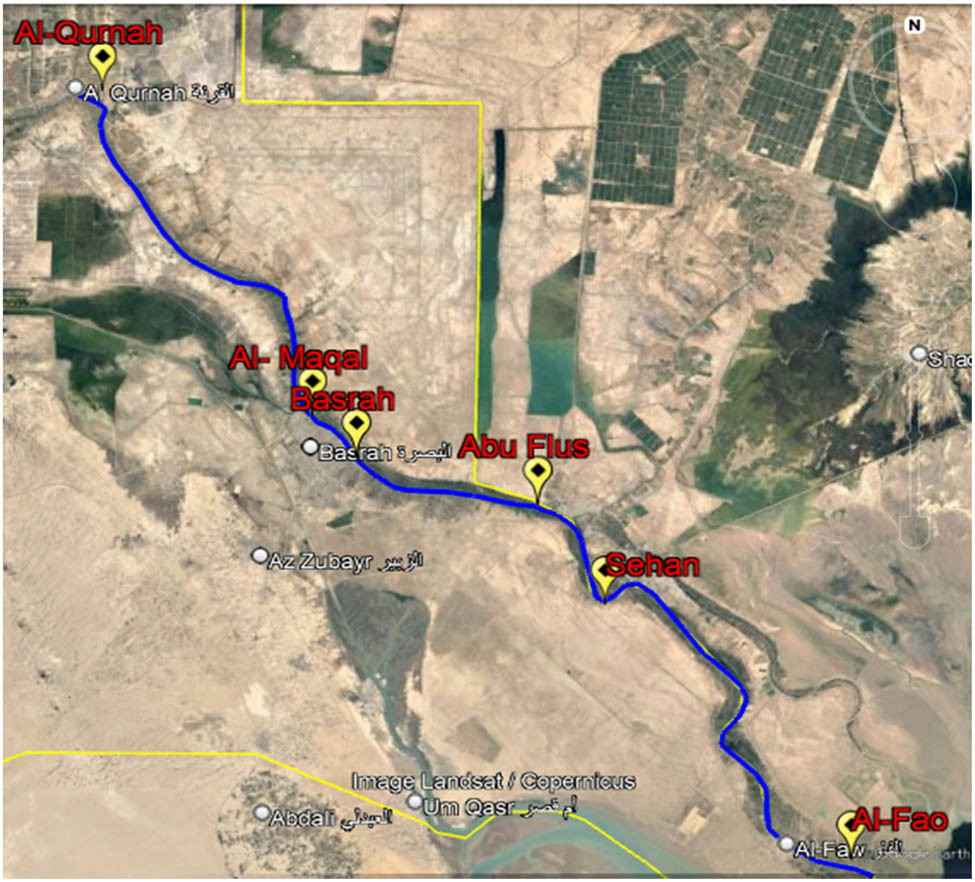
The Shatt Al-Arab River with sample locations.

Data for the year 2014 were used to develop the model. These data include cross-sections, daily flow and hourly stage hydrographs, temperature, conductivity, and TDS. Table 2 shows the location of the sampling stations along the River and the contribution of each data in the model building. A reported discharge from a separate model and a recorded hourly water stage for 2014 extended from 1 February up to 30 June were chosen as input upstream and downstream BC, respectively.

Table 2

Station’s location of data collected during the simulation time

Station	Location coordinate		Data type	Purpose
Station	E	N	Data type	Purpose
Al-Qurnah	47° 26.581′	31° 00.267′	Flow hydrograph	Upstream BC
Al-Maqal	47° 46.768′	30° 34.154′	Stage hydrograph	Verification
Abu Flus	48° 01.215′	30° 27.542′	Stage hydrograph	Calibration
Sehan	48° 11.623′	30° 19.587′	Stage hydrograph	Validation
Al-Fao	48° 30.256′	29° 57.879′	Stage hydrograph	Downstream BC

2.2 Basic model elements

The movement of the River has an impact on the physical transport and transmission of contaminants. Water motions at various scales and forms substantially impact the aggregation and distribution of nutrients, dissolved gases, temperature, and the distribution of microorganisms and plankton. As a result, the water quality model’s accuracy is highly dependent on the hydrodynamic model’s description of circulation. Therefore, three submodels were used sequentially to integrate the Shatt Al Arab River modeling: the hydrodynamic model of HEC-RAS, the heat model of WASP, and the eutrophication model of WASP.

2.2.1 Hydrodynamic model (HEC-RAS)

The study area, Shatt Al-Arab River, can be considered a shallow water surface because the width-to-depth ratio is more than 10 [28,29]. Therefore, the depth-averaged 2D hydrodynamic model is adopted to simulate the hydrological parameter variation in plain view (longitudinal and transverse direction) in HEC-RAS. However, computing the 2D Saint Venant equations [30,31] demands greater processing power, resulting in longer run durations. Furthermore, numerical instability of the equations can occur in areas of the 2D mesh where the flow path or depth profile changes abruptly. A refinement and shorter step will be required to avoid an unstable model [32].

2.2.2 Water temperature model (WASP)

WASP, developed by EPA, can simulate a wide range of contaminants and temperatures in a multidimensional geometry of rivers, estuaries, lakes, and reservoirs. One of the essential physical features of surface waterways is water temperature [33]. It is important in hydrodynamic and water quality research [2]. The temperature may be thought of as a measure of how much heat energy is kept in a water volume, and equation (1) describes the heat energy and temperature relationship [34]:

(1) H = V ( ρ w C p T ) = V C h ,

where H is the heat content, V is the volume, ρ is the density of water, and C _p is the specific heat of water 4,179 J/kg °C . At 25°C, T is the temperature and C _h is the heat concentration. The heat balance equation is obtained by substituting the component concentration in the mass equation with the heat concentration, which the heat model in WASP calculates. The surface heat exchange is computed using either a full heat balance [33] or equilibrium temperature and surface heat exchange coefficients. Water temperature sources and sinks related to surface heat exchange can be expressed as follows:

(2) ∂ V T ∂ t = H n A s ρ C p ,

where A _s is the surface area in m², t is the time in the day, and H _n is the net thermal energy flux (Watt/m²)

(3) H n = H s + H a + H e + H c − ( H sr + H ar + H br ) ,

where H _s is the shortwave solar radiation flux, H _a is the longwave radiation flux, H _e is the evaporation heat loss flux, H _c is the heat conduction flux, H _sr is the reflected short wave solar radiation, H _ar is the reflected long-wave radiation, and H _br is the back radiation from the water surface, also see Figure 2 for more explanation. Stephan Boltzmann’s fourth-power radiation law is utilized for H br [29,34]

(4) H br = ε σ ⁎ ( T s + 273 ) 4 ,

(5) H e = f ( W ) ( e s − e a ) ,

(6) H c = C c f ( W ) ( T s − T a ) ,

Shortwave solar radiation penetrates the surface and decays exponentially with depth according to Bears law:

(7) H s ( z ) = ( 1 − β ) H s e − η z .

To compute the heat flux components, the related parameters with typical values are listed in Table 3. Indeed, some models compute surface fluxes and regard bed energy transfer as insignificant [33].

Figure 2

Heat exchange processes.

Table 3

Parameters of heat flux components

Parameter	Meaning	Value for constant
ε	The emissivity of water	0.97
σ*	Stephan–Boltzmann constant	5.67 × 10⁻⁸W/m²/K⁴
T _s	Water surface temperature
f(W)	Evaporation wind speed function
e s	Saturation vapor pressure at the water surface
e a	Atmospheric vapor pressure
C _c	Bowen’s coefficient	0.47 mm Hg/EC
T _a	Air temperature
β	Fraction is absorbed in the water’s surface
η(K _e)	Extinction coefficient

The equilibrium temperature technique assumes that the net surface heat exchange is zero. This definition of the equilibrium temperature allows describing H _n as follows:

(8) H n = − K aw ( T w − T e ) ,

where K _aw is the coefficient of surface heat exchange, T _w is the water surface temperature, and T _e is the equilibrium temperature.

2.2.3 Eutrophication model

The core principle behind constructing a mass balance equation for a waterbody is to consider all materials entering and exiting the waterbody through direct material addition, such as runoff and loading, advection and dispersion transport processes, and physical, chemical, and biological changes [35]. The 2D mass transport equation is

(9) ∂ ( H C ) ∂ t + ∂ ( H u C ) ∂ x + ∂ ( H v C ) ∂ y = ∂ ∂ x H E x ∂ C ∂ x + ∂ ∂ y H E y ∂ C ∂ y + S L + S B + S K ,

where H is the water depth, C is the vertical average concentration of the water quality constituent, t is the time, u and v are longitudinal and lateral advective velocities, respectively, E _x and E _y are longitudinal and lateral diffusion coefficients, respectively, S _L is the direct loading rate, S _B is the boundary loading rate, S _K is the kinetic transformation rate; the source is positive, and the sink is negative. Depending on the types of state variables representation, different degrees of complexity have been recognized from simple Streeter–Phelps to nonlinear DO balance. Eight state variables that can contribute to eutrophication are included in Table 4 with their notations. It should be noted that all abbreviations appearing in the following equations have been explained in Appendix.

Table 4

Summary of EUTRO variables

	State variable	Notation	Concentration	Units
1	Ammonia nitrogen	NH₃	C1	mg N/L
2	Nitrate nitrogen	NO₃	C2	mg N/L
3	Inorganic phosphorus	PO₄	C3	mg P/L
4	Phytoplankton carbon	PHYT	C4	mg C/L
5	Carbonaceous BOD	CBOD	C5	mg O₂/L
6	Dissolved oxygen	DO	C6	mg O₂/L
7	Organic nitrogen	ON	C7	mg N/L
8	Organic phosphorus	OP	C8	mg P/L

2.2.3.1 Phosphorus

Inorganic phosphorus (IP) is consumed by phytoplankton for growth and assimilated into the biomass of phytoplankton. Endogenous respiration and nonpredatory mortality return phosphorus from the phytoplankton biomass as organic phosphorus (OP) in either dissolved or particulate form. OP is mineralized into IP at a dependency temperature rate [36].

Inorganic phosphorus (C ₃)
(10) S k 3 = k 83 θ 83 T − 20 C 4 K mPc + C 4 C 8 ︷ Mineralization + D P1 a pc ( 1 − f op ) C 4 ︷ Death − G P1 a pc C 4 ︷ Growth .
Organic phosphorus ( C 8 )

(11) S k8 = − k 83 θ 83 T − 20 C 4 K mPc + C 4 C 8 ︷ Mineralization + D P1 a pc f op C 4 ︷ Death − s 3 D ( 1 − f D 8 ) C 8 ︷ Settling .

2.2.3.2 Nitrogen

The nitrogen composition kinetics is similar to that of the phosphorus cycle. NH₃–N and nitrate are consumed by phytoplankton and assimilated into phytoplankton biomass for growth. The rate at which each is absorbed is controlled by its concentration concerning the total amount of inorganic nitrogen (NH₃–N plus nitrate) available. Through endogenous respiration and nonpredatory death, nitrogen is recovered from the phytoplankton biomass pool as dissolved and particulate organic nitrogen ON and NH₃–N. ON is mineralized to NH₃–N at a temperature-dependent rate, and NH₃–N is then transformed to nitrate at a temperature- and oxygen-dependent nitrification rate. In the absence of oxygen, nitrate may be transformed into nitrogen gas at a temperature and oxygen-dependent denitrification rate.

Ammonia nitrogen (C ₁):
(12) S k1 = k 71 θ 71 T − 20 C 4 K mPc + C 4 C 7 ︷ Mineralization + D P1 a nc ( 1 − f on ) C 4 ︷ Death − G P1 a nc P NH 3 C 4 ︷ Growth − k 12 θ 12 T − 20 C 6 K NIT + C 6 C 1 ︷ Nitrification .
Nitrate nitrogen (C ₂):
(13) S k2 = k 12 θ 12 T − 20 C 6 K NIT + C 6 C 1 ︷ Nitrification − G P1 a nc ( 1 − P NH 3 ) C 4 ︷ Growth − K 2 D θ 2 D T − 20 K NO 3 K NO 3 + C 6 C 2 ︷ Denitrification ,

(14) P NH 3 = C 1 C 2 ( K NO 3 + C 1 ) ( K NO 3 + C 2 ) + C 1 K NO 3 ( C 1 + C 2 ) ( K NO 3 + C 2 ) .
Organic nitrogen ( C 7 ):

(15) S k7 = − k 71 θ 71 T − 20 C 4 K mPc + C 4 C 7 ︷ Mineralization + D P1 a nc f on C 4 ︷ Death − s 3 D ( 1 − f D7 ) C 7 ︷ Settling .

2.2.4 Carbonaceous biochemical oxygen demand (CBOD)

In addition to man-made sources and natural runoff, detrital phytoplankton carbons generated by algal death are major sources of CBOD. The principal CBOD loss mechanisms are oxidation, settling, and denitrification. When phytoplankton dies, organic carbon is produced that can be oxidized. Recirculation of phytoplankton carbon to CBOD is represented by first-order expression and stoichiometric oxygen-to-carbon ratio 32/12.

(16) S k 5 = a oc k 1 d C 4 ︷ Death − k d θ d T − 20 C 6 K BOD + C 6 C 5 ︷ Oxidation − s 3 D ( 1 − f D 5 ) C 5 ︷ Settling − 5 4 32 14 K 2 D θ 2 D T − 20 K NO 3 K NO 3 + C 6 C 2 ︷ Denitrification .

2.2.4.1 DO

Reaeration and photosynthesis are the primary sources of DO. The principal DO loss mechanisms are oxidation, nitrification, sediment demand, and respiration:

(17) S k 6 = k 2 θ 2 T − 20 ( C s − C 6 ) ︷ Reaeration − k d θ d T − 20 C 6 K BOD + C 6 C 5 ︷ Oxidation − 64 14 k 12 θ 12 T − 20 C 6 K NIT + C 6 C 1 ︷ Nitrification − SOD D θ s T − 20 ︷ Sediment Demand + G P1 32 12 + 48 14 14 12 ( 1 − P NH 3 ) C 4 ︷ Phytoplankton growth − 32 12 k 1 R θ 1 R T − 20 C 4 ︷ Respiration .

2.2.4.2 Phytoplankton

The kinetics of phytoplankton plays a major role in eutrophication, impacting all other state variables. Where phytoplankton increases due to photosynthesis and are lost via respiration, death, and settling, Figure 3

(18) S k4 = ( G P1 − D P1 − K S4 ) P ,

where S _k4 is the reaction term, P is the phytoplankton population, G _P1 is the growth rate constant, D _P1 is the death plus respiration rate constant, and K _S4 is the settling rate constant.

Figure 3

Phytoplankton kinetics with related state variables.

Figure 4 depicts an overview of all transformation processes of the EUTRO system with related state variables.

Figure 4

A schematic diagram of the EUTRO process.

2.3 Models coupling and development

WASP does not support multidimensional hydrodynamics simulation, but its adaptable structure allows importing data from an external hydrodynamics model. External hydrodynamic models coupled to WASP through linkage files can anticipate transport information for complicated water bodies. Before the transformation process begins, it should be verified for quality. Consequently, this check is discussed in detail in the findings section.

2.3.1 External linkage

The transport information output of the hydrodynamic model, such as volumes, flows, velocity, etc., is reported in the result file, which was then extracted and utilized by WASP [37]. To make this connection properly, an external coupler written in Python v.3.7 (Figure 5), developed by [38], is used to link the two models via the development of an Application Program Interface (API). The various information in space and time that the hydrodynamic model sends to WASP contains segments’ volume, depth, velocity, temperature, and salinity.

Figure 5

Procedures of generated linkage file by Python code.

2.3.2 Segment description

The segment provides specific geometry information. To properly transmit data between the two model grids, the WASP segments were reproduced to HEC-RAS 2D cell boundaries by the hydrodynamic linkage file. It is preferable in modeling the mesh size of the HEC-RAS model (implicit finite-difference model) must be finer than the WASP model (explicit finite-difference model) to achieve convergence during the analysis [16]. In another ward, to prevent numerical errors for WASP, the HEC-RAS 2D computational grid cells should be collected for use in WASP (Figure 6).

Figure 6

Segments representation for HEC-RAS model (black mesh) and WASP model (blue mesh).

2.3.3 Model calibration

Tracers, whether synthetic or natural, such as salinity, chloride, dye, or heat, are frequently employed to calibrate the dispersion coefficients for a model network. A chemical tracer is a nonreactive (conservative tracer) chemical conveyed through a body of water. The first step in modeling more complicated water quality factors is to set up and calibrate a tracer. Five common statistical error methods have been adopted in Water Resource Data Base (WRDB) calibration to give an adequate view for accepting or refusing the model outputs. These methods were coefficient of determination (r ²), mean absolute error (MAE), root-mean-square error (RMSE), normalized RMSE (N RMSE), and index of agreement (d) [39,40,41,42,43].

3 Results overview and discussion

3.1 HEC-RAS results

Calibration of HEC-RAS 2D output for water surface elevation is done by changing Manning’s roughness coefficient (n). Three distinct values of “n” were considered: n = 0.02, n = 0.025, and n = 0.035; then chose, an appropriate “n” value that gives allowable criteria ranges between simulated and observed water stages. As it appears from Table 5, there is an acceptable convergence between the calculated and measured values at n value is equal to 0.025.

Table 5

Model performance statistic during calibration

‘n’ value	Statistical analysis method
	RMSE	MAE	NSE
0.02	0.182	0.144	0.806
0.025	0.176	0.140	0.836
0.035	0.178	0.145	0.812

3.2 External linkage results

Figure 7a and b illustrates the flow pairs for adjacent HEC-RAS cells and WASP segments, respectively. It is noted that cell/segment 5,623 has flow exchange with 3 of the neighbor cells/segments (3,719, 5,622, and 5,624), which are listed in the WASP table. This indicates that a good transformation results from the flow path through the River network. Another proof of successful coupling is an apparent match of the WASP model’s results of velocity and depth (Figure 7d and f), with the corresponding HEC-RAS model’s results (Figure 7c and e). More details of the hydrodynamic model results transferred by the linkage file are shown in Figure 8. This figure illustrates the depth variation affected by tidal phenomena at different locations along the Shatt Al Arab River. These graphs were constructed by WRDB software. Now, WASP is ready to be initiated for contaminants simulation.

Figure 7

A variable data transferred from HEC-RAS to WASP: (a) flow pairs of cells as appeared in the HEC-RAS window, (b) flow pairs of segments as appeared in the WASP window, (c) velocity profile of cell No. 1 as HEC-RAS results, (d) velocity profile of segment No. 1 as linking WASP results, (e) depth profile of cell No. 1 as HEC-RAS results, and (f) depth profile of segment No. 1 as linking WASP results.

Figure 8

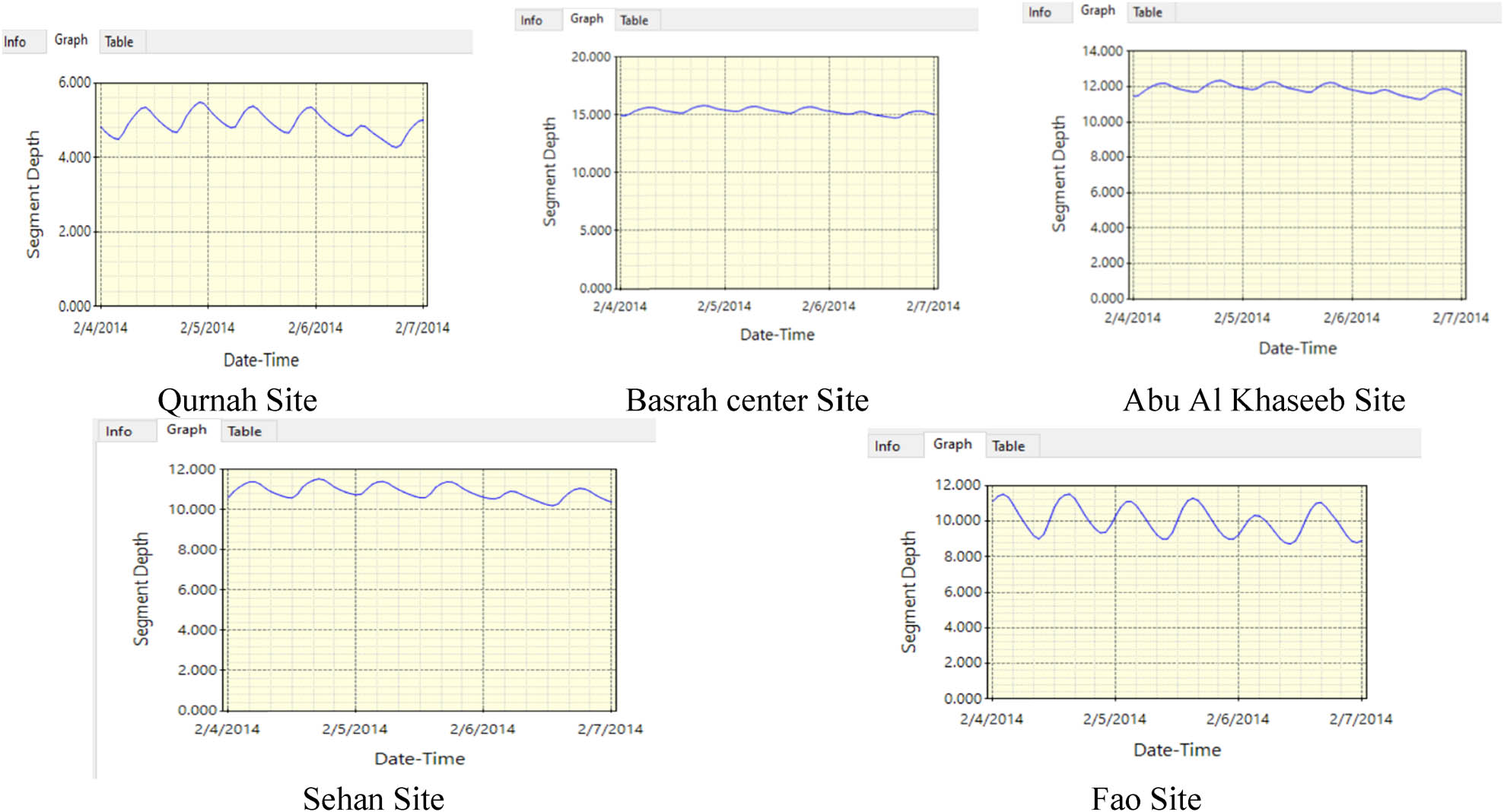
Depth variation at different stations along the Shatt Al Arab River. Qurnah Site, Basrah center Site, Abu Al Khaseeb Site Sehan Site, Fao Site.

3.3 WRDB calibration results

Figures 9 and 10 illustrate calibration results for Basrah and Sehan stations, respectively. It can be seen that the summary of the statistical analysis appears on the right side of each figure. This part illustrates statistical parameters such as mean, min, max, and standard deviation for simulated and observed data. Also, it describes the results of r ², MAE, RMSE, NRMSE, and d. The result of r ² (0.85), NRMSE (0.125), and d (0.88) gave an acceptable convergence between simulated and observed values at the Basrah center station. While the result of methods MAE and RMSE gave overestimation. Similarly, it can be recognized same behavior at Sehan station. The left part of Figures 9 and 10 shows the graphical representation of simulated and observed data for time series, probability, and linear fit to make a direct comparison during calibration.

Figure 9

Calibration statistics at the Basrah center station.

Figure 10

Calibration statistics at the Sehan station.

3.4 EUTRO model results

A 2D concentration distribution is displayed on the window of the WRDBGIS software as a colored spatial grid through the simulation time, as shown in Figures 11 and 12. Figure 11 shows TDS concentration variation through a tidal period at the downstream end of the River, where the value increased gradually during the rising phase to extend the high concentration value for approximately 10 km from the downstream end, then decreased through the falling phase. After proceeding with the modeling process, it is seen that the penetration distance is increasing with time, where at date and time (2/16/2014 16:00), it is found to be 22.4 km with a TDS range of 9,000–10,000 mg/L (Figure 12a), and at date and time (3/17/2014 03:00), it is found to be 28.7 km with a concentration range of 8,000–9,000 mg/L (Figure 12b). And the recorded distances of penetration were 35.2 km with a range of 8,000–9,000 mg/L and 38.2 km with a concentration range of 7,000–8,000 mg/L at 2/26/2014 00:00 and 2/26/2014 22:00, respectively (Figure 12c and d).

Figure 11

TDS concentration variation through a tidal period at the downstream end.

Figure 12

Spatial grid TDS concentration distribution. (a) penetration distance with higher concentration range at 2/16/2014 16:00, (b) penetration distance with higher concentration range at 3/17/2014 03:00, (c) penetration distance with higher concentration range at 2/26/2014 00:00, and (d) penetration distance with higher concentration range at 2/26/2014 22:00.

Another way to display the WASP results is an x/y plot as a time series variation for the constituents. It is possible to choose several segments (cells) along the river to show the variation of TDS concentration at different stations, as shown in Figure 13. From this figure, the concentration of TDS increased toward the estuary. At the Qurnah station, the TDS ranged from 500 to 1,500 and from 1,500 to 2,000 mg/L at the Basrah station, while at the Sehan station was 1,500–3,000 mg/L. Moreover, one can illustrate the transversal distribution by selecting segments that lie on the same line across the river; Figure 14 is an example for the Fao station since the values at the river center, left, and right bank are different.

Figure 13

A variation of TDS concentration at different stations.

Figure 14

Transverse distribution of TDS concentration at the Fao station.

4 Conclusion

This article aims to develop a comprehensive water quality model of the Shatt Al Arab River south of Iraq by linking HEC-RAS with WASP. A variety of software techniques has sequentially been used. This software includes GIS for DEM modification, HEC-RAS for the hydrodynamic model, Python code with PyCharm to run the external coupler, WASP software for advective and dispersive contaminant transport, and finally, WRDB/WRDBGIS software for full calibration process and results display. Therefore, three submodels were used sequentially to integrate the Shatt Al Arab River modeling: the hydrodynamic model of HEC-RAS, the heat model of WASP, and the eutrophication model of WASP. Data for the year 2014 were used to develop the model. These data include cross-sections, daily flow and hourly stage hydrographs, temperature, conductivity, and TDS. A reported discharge from a separate model and a recorded hourly water stage for 2014 extended from 1 February up to 30 June were chosen as input upstream and downstream BC, respectively. The study area, Shatt Al-Arab River, can be considered a shallow water surface because the width-to-depth ratio is more than 10; therefore, the depth-averaged 2D hydrodynamic model is adopted. Eight state variables (NH₃, NO₃, PO₄, PHYT, CBOD, DO, ON, and OP) that can contribute to eutrophication are included with their equations of kinetic reaction. The results indicate a good flow path transformation through the River network. The calibration tool can give a clear vision to make the right decision about the model’s accuracy.

Conflict of interest: The authors state no conflict of interest.
Data availability statement: Most datasets generated and analyzed in this study are included in this submitted manuscript. The other datasets are available on reasonable request from the corresponding author with the attached information.

Appendix

Description of abbrivations used in the study

Notation	Description	Units
a _oc	Oxygen-to-carbon ratio	mg O₂/mg C
a _nc	Nitrogen-to-carbon ratio	mg N/mg C
a _pc	Phosphorus-to-carbon ratio	mg P/mg C
k _d	Deoxygenation rate @ 20°C	Day⁻¹
θ _d	Deoxygenation temperature coefficient	—
K _BOD	Half saturation constant for oxygen limitation	mg O₂/L
k ₁₂	Nitrification rate @ 20°C	Day⁻¹
θ ₁₂	Nitrification temperature coefficient	—
K _NIT	Half saturation constant for oxygen limitation	mg N/L
K _2D	Denitrification rate @ 20°C	Day⁻¹
θ _2d	Denitrification temperature coefficient	—
K No 3	Half saturation constant for oxygen limitation (Michaelis constant)	mg N/L
G _p1	Phytoplankton growth rate	Day⁻¹
K _1R	Phytoplankton respiration rate @ 20°C	Day⁻¹
θ _1R	Phytoplankton temperature coefficient	—
SOD	Sediment oxygen demand	Day⁻¹
θ _s	Temperature coefficient	—
k ₂	Reaeration rate @ 20°C	Day⁻¹
θ ₂	Reaeration temperature coefficient	—
c _s	Dissolved oxygen demand	mg O₂/L
f _D3	Fraction-dissolved inorganic phosphorus	—
f _D5	Fraction-dissolved CBOD	—
f _D7	Fraction-dissolved organic nitrogen	—
f _D8	Fraction-dissolved organic phosphorus	—
v _s3	Organic matter settling velocity	m/day
v _s5	Inorganic matter settling velocity	m/day
C ₁	Ammonia nitrogen NH₃	mg N/L
C ₂	Nitrate nitrogen NO₃	mg N/L
C ₃	Inorganic phosphorus	mg P/L
C ₄	PHYT	mg C/L
C ₅	Carbonaceous BOD CBOD	mg O₂/L
C ₆	Dissolved oxygen	mg O₂/L
C ₇	Organic nitrogen	mg N/L
C ₈	Organic phosphorus	mg P/L
K _e	Extinction coefficient	m⁻¹
D	Segment depth	m
T	Water temperature	C
f	Fraction of day that is daylight	—
I _s	Average daily surface solar radiation	langleys/day
Z	Zooplankton population	mg C/L
K _1c	Maximum growth rate	Day⁻¹
Δ _1c	Temperature coefficient	—
K _1R	Endogenous respiration @ 20°C	Day⁻¹
θ _1R	Endogenous respiration Temperature coefficient	—
K _1D	Death rate	Day⁻¹
K _1G	Grazing rate	1/mg c-day
k ₇₁	Mineralization rate of organic nitrogen @ 20°C	Day⁻¹
θ ₇₁	Mineralization rate temperature coefficient	—
k ₈₃	Mineralization rate of organic phosphorus @20°C	Day⁻¹
θ ₈₃	Mineralization rate temperature coefficient	—
K _mpc	Half saturation for phytoplankton limitation of Phosphorus	mg C/L
f _OP	Fraction of dead and respired phytoplankton to inorganic Phosphorus nitrogen	—
1 − f _OP	Fraction of dead and respired phytoplankton to inorganic Phosphorus nitrogen	—
f _ON	Fraction of dead and respired phytoplankton to organic nitrogen	—
1 − f _ON	Fraction of dead and respired phytoplankton to ammonia nitrogen	—
P NH 3	Preference for ammonia uptake	—

References

[1] Tsakiris G, Alexakis D. Water quality models: An overview. European Water. 2012;37:33–46.Suche in Google Scholar

[2] Ji ZG. Hydrodynamics and water quality: modeling rivers, lakes, and estuaries. USA: John Wiley & Sons; 2017.10.1002/9781119371946Suche in Google Scholar

[3] Lindenschmidt KE, Sabokruhie P, Rosner T. Modelling transverse mixing of sediment and vanadium in a river impacted by oil sands mining operations. J Hydrol Reg Stud. 2022;40:101043. 10.1016/j.ejrh.2022.101043.Suche in Google Scholar

[4] Orlob GT. Mathematical modeling of water quality: Streams, lakes and reservoirs. Vol. 12. Chichester, UK: John Wiley & Sons; 1983.Suche in Google Scholar

[5] Liu CC, Lin P, Xiao H. Water Environment Modeling. Boca Raton, Florida: CRC Press; 2021.10.1201/9781003008491Suche in Google Scholar

[6] Bai J, Zhao J, Zhang Z, Tian Z. Assessment and a review of research on surface water quality modeling. Ecol Modell. 2022;466:109888. 10.1016/j.ecolmodel.2022.109888.Suche in Google Scholar

[7] Fu B, Merritt WS, Croke BF, Weber TR, Jakeman AJ. A review of catchment-scale water quality and erosion models and a synthesis of future prospects. Environ Modell Soft. 2019;114:75–97. 10.1016/j.envsoft.2018.12.008.Suche in Google Scholar

[8] Ramos-Ramírez LÁ, Guevara-Luna MA, Chiriví-Salomón JS, Muñoz-Nieto DM. Simulation of Cr-III dispersion in the High Bogotá River Basin using the WASP model. Revista Facultad de Ingeniería Universidad de Antioquia. 2020;97:30–40. 10.17533/udea.redin.20191155.Suche in Google Scholar

[9] Marvin J, Wilson AT. One dimensional, two dimensional and three dimensional hydrodynamic modeling of a Dyked Coastal River in the bay of Fundy. J Water Manage Modell. 2016;25:404. 10.14796/JWMM.C404.Suche in Google Scholar

[10] Alam A, Badruzzaman A, Ali MA. Assessing effect of climate change on the water quality of the Sitalakhya river using WASP model. J Civ Eng. 2013;41:21–30.Suche in Google Scholar

[11] Chuersuwan N, Nimrat S, Chuersuwan S. Empowering water quality management in Lamtakhong River basin, Thailand using WASP model. Res J App Sci Eng Technol. 2013;6(23):4485–91.10.19026/rjaset.6.3456Suche in Google Scholar

[12] Yen CH, Chen KF, Sheu YT, Lin CC, Horng JJ. Pollution source investigation and water quality management in the Carp Lake watershed, Taiwan. Clean Soil Air Water. 2012;40(1):24–33. 10.1002/clen.201100152.Suche in Google Scholar

[13] Datta AR, Kang Q, Chen B, Ye X. Fate and transport modelling of emerging pollutants from watersheds to oceans: a review. Adv Mar Biol. 2018;81:97–128. 10.1016/bs.amb.2018.09.002.Suche in Google Scholar PubMed

[14] Chueh YY, Fan C, Huang YZ. Copper concentration simulation in a river by SWAT-WASP integration and its application to assessing the impacts of climate change and various remediation strategies. J Environ Manage. 2021;279:111613. 10.1016/j.jenvman.2020.111613.Suche in Google Scholar PubMed

[15] Quijano JC, Zhu Z, Morales V, Landry BJ, Garcia MH. Three-dimensional model to capture the fate and transport of combined sewer overflow discharges: A case study in the Chicago Area Waterway System. Sci Total Environ. 2017;576:362–73. 10.1016/j.scitotenv.2016.08.191.Suche in Google Scholar PubMed

[16] Defne Z, Spitz FJ, DePaul V, Wool TA. Toward a comprehensive water-quality modeling of Barnegat Bay: development of ROMS to WASP coupler. J Coastal Res. 2017;78(10078):34–45. 10.2112/SI78-004.1.Suche in Google Scholar

[17] Yao H, Zhuang W, Qian Y, Xia B, Yang Y, Qian X. Estimating and predicting metal concentration using online turbidity values and water quality models in two rivers of the Taihu Basin, Eastern China. PLoS One. 2016;11(3):e0152491. 10.1371/journal.pone.0152491.Suche in Google Scholar PubMed PubMed Central

[18] Yin Z, Seo D. Water quality modeling of the Ara Canal, using EFDC-WASP model in series. J Korean Soc Environ Eng. 2013;35(2):101–8.10.4491/KSEE.2013.35.2.101Suche in Google Scholar

[19] Ernst MR, Owens J. Development and application of a WASP model on a large Texas reservoir to assess eutrophication control. Lake Reservoir Manage. 2009;25(2):136–48. 10.1080/07438140902821389.Suche in Google Scholar

[20] Wool TA, Davie SR, Rodriguez HN. Development of three-dimensional hydrodynamic and water quality models to support total maximum daily load decision process for the Neuse River Estuary. North Carolina. J Water Resour Plan Manag. 2003;129(4):295–306. 10.1061/∼ASCE!0733-9496∼2003!129:4∼295!.Suche in Google Scholar

[21] Rodriguez HN, Peene SJ. Development of a dissolved oxygen TMDL for Brunswick river using a 2-D hydrodynamic and water quality model. USA: Georgia Institute of Technology; 2001.Suche in Google Scholar

[22] Kareem HH, Alkatib AA. Future short-term estimation of flowrate of the Euphrates river catchment located in Al-Najaf Governorate, Iraq through using weather data and statistical downscaling model. Open Eng. 2022;12(1):129–41. 10.1515/eng-2022-0027.Suche in Google Scholar

[23] Hamdan ANA, Dawood AS. Neural network modelling of Tds concentrations in Shatt Al-Arab river water. Eng TechJ. 2016;34(2):334–45.10.30684/etj.34.2A.12Suche in Google Scholar

[24] Hamdan ANA. Simulation of salinity intrusion from arabian Gulf to Shatt Al-Arab River. Basrah J Eng Sci. 2015;16(1):28–32.10.33971/bjes.16.1.5Suche in Google Scholar

[25] Abdullah AD. Modelling approaches to understand salinity variations in a highly dynamic tidal river, in the academic board of the UNESCO-IHE Institute for Water Education. Netherlands: Delft University of Technology; 2016.10.1201/9781315115948Suche in Google Scholar

[26] Hamdan A, Dawood A, Naeem D. Assessment study of water quality index (WQI) for Shatt Al-arab River and its branches, Iraq. In MATEC Web of Conferences. EDP Sciences; 2018.10.1051/matecconf/201816205005Suche in Google Scholar

[27] Hamdan ANA, Al-Mahdi AAJ, Mahmood AB. Modeling the effect of sea water intrusion into Shatt Al-Arab River (Iraq). J Univ Babylon Eng Sci. 2020;28:210–24.Suche in Google Scholar

[28] Al-Azzawi SN, Khudair KM. A finite element model to simulate the hydrodynamics of Shatt Al- Basrah Canal and Khour Al-Zubair Estuary. J Eng. 2001;7(2):283–308.Suche in Google Scholar

[29] Krenkel P. Water quality management. Technology & Engineering. New York: Elsevier; 2012.Suche in Google Scholar

[30] Behzadi F, Wasti A, Steissberg TE, Ray PA. Vulnerability assessment of drinking water supply under climate uncertainty using a river contamination risk (RANK) model. Environ Modell Soft. 2022;150:105294. 10.1016/j.envsoft.2021.105294.Suche in Google Scholar

[31] Brunner G. HEC-RAS, river analysis system hydraulic reference manual, Version 6.0. Report Number CPD-69, Hydrologic Engineering Center. Davis, California: US Army Corps of Engineers; 2020.Suche in Google Scholar

[32] Quirogaa VM, Kurea S, Udoa K, Manoa A. Application of 2D numerical simulation for the analysis of the February 2014 Bolivian Amazonia flood: Application of the new HEC-RAS version 5. Ribagua. 2016;3(1):25–33. 10.1016/j.riba.2015.12.001.Suche in Google Scholar

[33] Dugdale SJ, Hannah DM, Malcolm IA. River temperature modelling: A review of process-based approaches and future directions. Earth Sci Rev. 2017;175:97–113. 10.1016/j.earscirev.2017.10.009.Suche in Google Scholar

[34] Wool TA, Ambrose Jr R, Martin J. WASP8 temperature model theory and user’s guide. Supplement to water quality analysis simulation program (WASP) user documentation. Washington, DC: U.S. Environmental Protection Agency Office of Research and Development; 2008.Suche in Google Scholar

[35] Di Toro DM, Fitzpatrick JJ, Thomann RV. Documentation for water quality analysis simulation program (WASP) and model verification program (MVP). Duluth, Minnesota: U.S. Environmental Protection Agency Office of Research and Development; 1983.Suche in Google Scholar

[36] Kim JS, Seo IW, Lyu S, Kwak S. Modeling water temperature effect in diatom (Stephanodiscus hantzschii) prediction in eutrophic rivers using a 2D contaminant transport model. J Hydro Environ Res. 2018;19:41–55. 10.1016/j.jher.2018.01.003.Suche in Google Scholar

[37] Wool T, Ambrose Jr RB, Martin JL, Comer A. WASP 8: The next generation in the 50-year evolution of USEPA’s water quality model. Water. 2020;12(5):1398. 10.3390/w12051398.Suche in Google Scholar PubMed PubMed Central

[38] Shabani A, Woznicki SA, Mehaffey M, Butcher J, Wool TA, Whung PY. A coupled hydrodynamic (HEC‐RAS 2D) and water quality model (WASP) for simulating flood‐induced soil, sediment, and contaminant transport. J Flood Risk Manag. 2021;14(4):e12747. 10.1111/jfr3.12747.Suche in Google Scholar PubMed PubMed Central

[39] Rhomad H, Khalil K, Neves R, Sobrinho J, Dias JM, Elkalay K. Three-dimensional hydrodynamic modelling of the Moroccan Atlantic coast: A case study of Agadir bay. J Sea Res. 2022;188:102272. 10.1016/j.seares.2022.102272.Suche in Google Scholar

[40] Pandey VK, Panda RK. Calibration and Validation of HEC-RAS Model for Minor Command in Coastal Region. Int J Curr Microbiol App Sci. 2020;9(2):664–78. 10.20546/ijcmas.2020.902.082.Suche in Google Scholar

[41] Garcia-Feal O, Cea L, Gonzalez-Cao J, Domínguez JM, Gomez-Gesteira M. IberWQ: A GPU accelerated tool for 2D water quality modeling in rivers and estuaries. Water. 2020;12(2):413. 10.3390/w12020413.Suche in Google Scholar

[42] Willmott CJ, Robeson SM, Matsuura K. A refined index of model performance. Int J Climatol. 2012;32(13):2088–94. 10.1002/joc.2419.Suche in Google Scholar

[43] Al-Waeli LK, Sahib JH, Abbas HA. ANN-based model to predict groundwater salinity: A case study of West Najaf–Kerbala region. Open Eng. 2022;12(1):120–8. 10.1515/eng-2022-0025.Suche in Google Scholar

Received: 2022-11-28

Revised: 2023-01-29

Accepted: 2023-02-07

Published Online: 2023-06-26

This work is licensed under the Creative Commons Attribution 4.0 International License.

Artikel in diesem Heft

https://doi.org/10.1515/eng-2022-0416

Schlagwörter für diesen Artikel

hydrodynamic modeling; water quality modeling; HEC-RAS; WASP; WRDB; external coupling; Shatt Al-Arab modeling

Creative Commons

BY 4.0