Assessment of the impacts of land use/land cover change on water resources in the Diyala River, Iraq

Ahmed Sagban Khudier; Ahmed Naseh Ahmed Hamdan

doi:10.1515/eng-2022-0456

Article Open Access

Assessment of the impacts of land use/land cover change on water resources in the Diyala River, Iraq

Ahmed Sagban Khudier and Ahmed Naseh Ahmed Hamdan

Published/Copyright: October 10, 2023

Published by

Become an author with De Gruyter Brill

Submit Manuscript Author Information

From the journal Open Engineering Volume 13 Issue 1

Abstract

In this study, the analysis was carried out concerning previous changes in land use/land cover (LULC) for 2 years, 2000 and 2020, and their impact on water resources in the Diyala River Watershed in Iraq was assessed. The Soil and Water Assessment Tool (SWAT) model is a hydrological model used to perform the hydrological modeling process for LULC maps. The data for LULC were collected using the Landsat satellite with a resolution of 30 m, and it was classified using geographical information systems (ArcGIS). Using the confusion matrix, the accuracy of the maps for the years 2000 and 2020 was evaluated, the overall accuracy was more than 90%, and the kappa coefficient (ka) was more than 88%, which indicates the accuracy of the classification and is ideal for use in modeling work. SUFI-2 included with the SWATCUP program was used to perform the calibration and the results were validated for the outflow of the two gauging stations within the study area of Hemren station and Derbendikhan station as a monthly time step for a baseline map LULC 2000, in the period 1996–2020 with 4 years as warm up. Coefficient of determination (R ²), Nash–Sutcliffe efficiency (NSE), and percent bias (Pbias) were used, which were the most common indicators for evaluating the performance of the statistical model. The results indicated that the values of R ² during the calibration and validation processes were (0.84–0.88) and (0.85–0.87), respectively; the NSE was (0.87–0.85), and the Pbias was (4.2–6.8)% and (5.8 to −4.1)%, respectively. Therefore, the calibration and verification results were good and satisfactory. In addition to the two LULC maps for 2000 and 2020, the parameters of the modified SWAT model were utilized to estimate the effects on the Diyala River Basin. The study found that LULC change affects basins and sub-basins differently. At the basin, hydrological parameters were largely unaffected by LULC changes. However, at the sub-basin level, the water yield and the surface runoff were changed between (−6.45 to 4.67)% and (−2.9 to 9.88)%, respectively.

Keywords: Arc SWAT model; Diyala River; hydrological model; LULC changes

1 Introduction

By altering land use and water flow routes, human activities are causing dangerous shifts in aquatic ecosystems and their resources [1]. Land use/land cover changes (LULCC) affect components of the hydrological cycle [1], which is the main factor controlling the management of water resources and hydrological models [2]. The land use/land cover (LULC) is the biophysical lid on the earth’s surface that has a substantial effect on the water balance and geomorphologic processes of the natural world, and its categories could be general agricultural lands, settled areas, shrublands, barren lands, etc. [3,4]. The effect of LULC on hydrological processes and water resources has been seen in the last few decades, as urbanization, agricultural practices, and climate change have had a clear impact on evapotranspiration, percolation, surface runoff (SURQ), and water yield [5,6].

LULCC has been predicted to have more serious impacts than climate change by 2025; therefore, we must have a clear understanding of how LULC has changed in the past, present, and future. Consequently, by learning more about how LULC impacts hydrological processes, policymakers may be able to make more sustainable and effective decisions when carrying out watershed improvement and development plans [4].

The use of satellite remote sensing for past images and geographical information systems (GISs) provides a substantial base in the administration of the surface of the earth by supplying information on the spatial–temporal in LULCC, particularly in large, unmonitored areas, and also helps to draw its effects on the parameters of hydrological models such as SURQ, evapotranspiration (ET), percolation (PER), water yield (WYLD), and lateral flow (LATQ) [2,7], so the hydrologic models allow comparison of basinal changes in hydrological components with LULCC [7]. Soil and Water Assessment Tool (SWAT) is one of the most important hydrological models in the world, and it has been used in many previous hydrological studies [7,8] and in this study.

SWAT is a GIS-based hydrological model that is easy to execute, almost distributed and has a suitable foundation for studying the effects of LULC on water quantity and quality in the watershed areas [6].

The SWAT model has been used in different studies to evaluate how climate changes affect sediment yields [9,10,11], the impact of LULCC on hydrological modeling [12,13,14], water balance in watersheds [15,16,17], impacts of LULCC on water resources [18,19], SURQ forecasting [20], and water quality [21,22,23]. Consequently, this study aids officials in understanding regional changes and making the necessary decisions to manage water resources for plans.

This study aims to identify the changes in LULC and its impact on hydrological variables such as SURQ, PER, ET, WYLD, and LATQ at the basin and sub-basin levels using the SWAT model and GIS software for the Diyala River Watershed (DRW), Iraq.

2 Study area

The Diyala River represents a significant water source for the middle and south of Iraq and is one of the main tributaries of the Tigris River [23]. The main source of the River is the Iranian mountains. It extends towards the Iraqi border, where its location is between latitude 33°57′–35°50′ and longitude 44°30′–47°50′ [24], along the two dams of River, Hemren dam (HD) and Derbendikhan dam (DD), as shown in Figure 1. The DRW covers 25,652 km², discharging to the south of Baghdad city through the Tigris River [25].

Figure 1

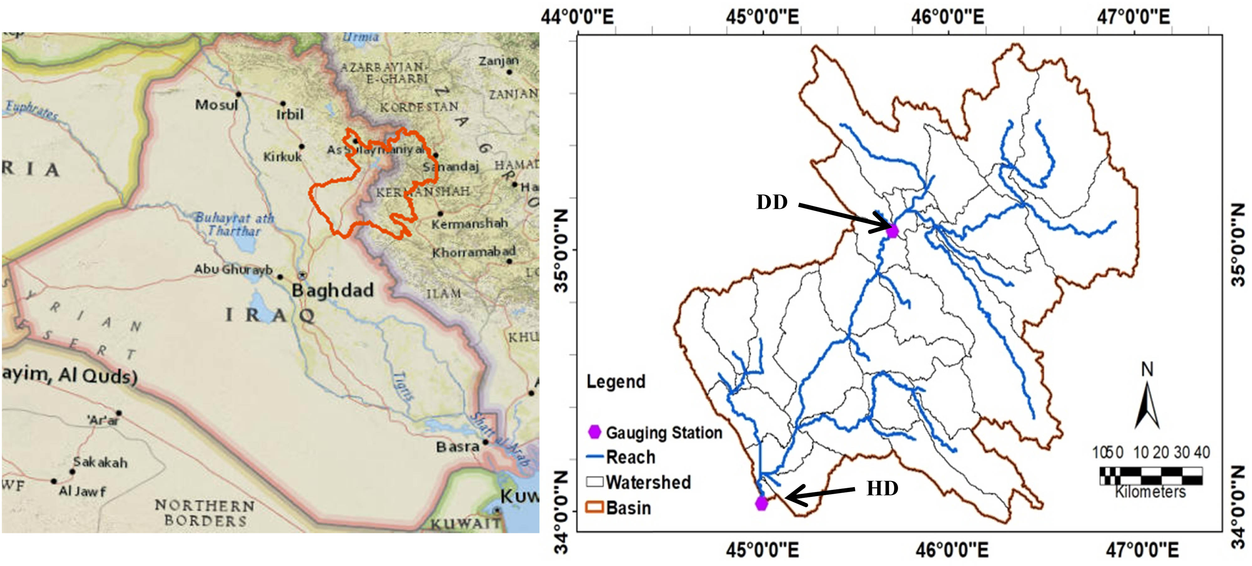
Location map for the watershed of Diyala River.

The basin is elevated from 46 to 3,351 m above sea water level. Domestic use follows irrigation projects as the most significant users of water in DRW [26,27]. The average monthly discharge for the basin from 1996 to 2020 reached 97.5 m³/s (Administration of HD and DD, Iraq, 2022, unpublished data). The annual precipitation in the basin was 320 mm and almost occurred from December to March, while the average temperature was 20°C (Iraqi Meteorological Organization, Iraq, 2022, unpublished data).

3 Methodology

There are two main components to the methodology: 1) classification of LULC and then the discovery changes from 2000 up to 2020 using GIS and Landsat satellite images; 2) modeling of hydrological using the SWAT model to find the impacts of previous changes of LULC on hydrological components.

3.1 Image classification operation

For the study area, the LULC maps to the years 2000 and 2020 were obtained from satellite Landsat images downloaded from the site arthexplorer.usgs.gov with geospatial tagged Image file format (Geo TIFF).

The acquisition date for the imagery in the year 2000 is 20 September, while for the year 2020 it was 10 October, with a spatial resolution of the imagery being 30 m and a path/row equal to 169/53.

Each image has a maximum cloud coverage of 10%. Then, it was georeferenced to the World Geodetic System for 1984 as a datum and Universal Transverse Mercator (UTM) Zone 38 North coordinate system.

Using the composite band button in the window image analysis, each band’s image was layer stacked, and then the image stacked was clipped by DRW to extract the study area. The popular bands of the datasets are Green, Red, Blue, and Near-infrared, which are used to reclassify the LULC [2].

The basic step in the process of classification is to collect a set of a group of samples from the study area. A comparison is made between the LULC found in the field and the one map in the image for the same location, and the precision of the statistics Assessment collects a set of all study area [2,28].

The error matrix was used to check the precision for the classification process proportional to prediction data and the accuracy of image classification; the kappa coefficient (ka) became the standard measure to evaluate the accuracy [16]. User’s accuracy (UA), producer’s accuracy (PA), overall accuracy (OA), and the ka can be calculated using the following equations:

(1) OA = 1 N ∑ i = 1 r nii ,

(2) PA = nii ni column ,

(3) UA = nii ni row ,

(4) ka = N ∑ i = 1 r nii − ∑ i = 1 r ni column * ni row N 2 − ∑ i = 1 r ni column * ni row ,

where i is the number of pixels classified correctly in an LULC classification; N is the all pixels number in the error matrix; r is the rows number; and ni row and ni column are the rows (predicted classes) and column (reference data) total.

3.2 Hydrological model in SWAT

The hydrological model is a simplified representation of the real-world system. The better model gives results near reality with minimum parameters and the least complicated [29]. The model of SWAT was developed by the United States Department of Agriculture (USDA) to forecast the SURQ, sediment yield, and effect of LULCC on the water resources in a vast watershed area [7].

In the SWAT model, the hydrological model includes data input, model setup, sensitivity analysis after the run model, calibration and validation, and estimation of performance [17].

The great basin is divided using SWAT into many tiny sub-basins, and then all the sub-basins are separated into many hydrological response units (HRUs). HRU is part of the sub-basin, with the same land use, soil texture, and slope. In the present study, the surface flow is estimated from the soil conservation services (SCS) curve number (CN) method with daily rainfall, a variable storage method used to route surface flow from any sub-basin through the network of River to the major basin outlets at HD and DD, the Penman–Monteith method was used to estimate potential evapotranspiration (PET).

In the SWAT model simulation, the hydrologic cycle is represented by [6,30]:

(5) SW t = SW 0 + ∑ i = 1 t ( R day − Q surf − Ea − W seep − Qgw ) ,

where SW_t is the final water content of the soil (mm), SW₀ is the initial water content of the soil on the day 1 (mm), t is the time (days), R _day is the amount of precipitation on day 1 (mm), Q _surf is amounting of SURQ on day 1 (mm), Ea is amounting of evapotranspiration on day 1 (mm), W _seep represents the amount of water that enters the vadose zone from the soil profile on day 1 (mm), and Qgw is the amount of return flow on day 1 (mm).

4 Input data

All the input datasets are described in the following sections.

4.1 A digital elevation model (DEM)

The spatial resolution (30 × 30) m was downloaded from the website https://earth explorer.usgs.gov, which was taken from the Shuttle Radar Topography Mission (Figure 2a). It is utilized for delineating and dividing the basin into sub-basins. This study divided the basin into 33 sub-basin numbers, varying from 2.8 km² in sub-basin number 8 to 2,560 km² in sub-basin number 24. The sub-basins are connected spatially, and the whole streamflow goes through an outlet sited in sub-basin 33. Several recent studies have shown that dividing the basin into too many sub-basins may not give better results for the model forecasting if the spatial weather difference parameters are obtained without errors [7].

Figure 2

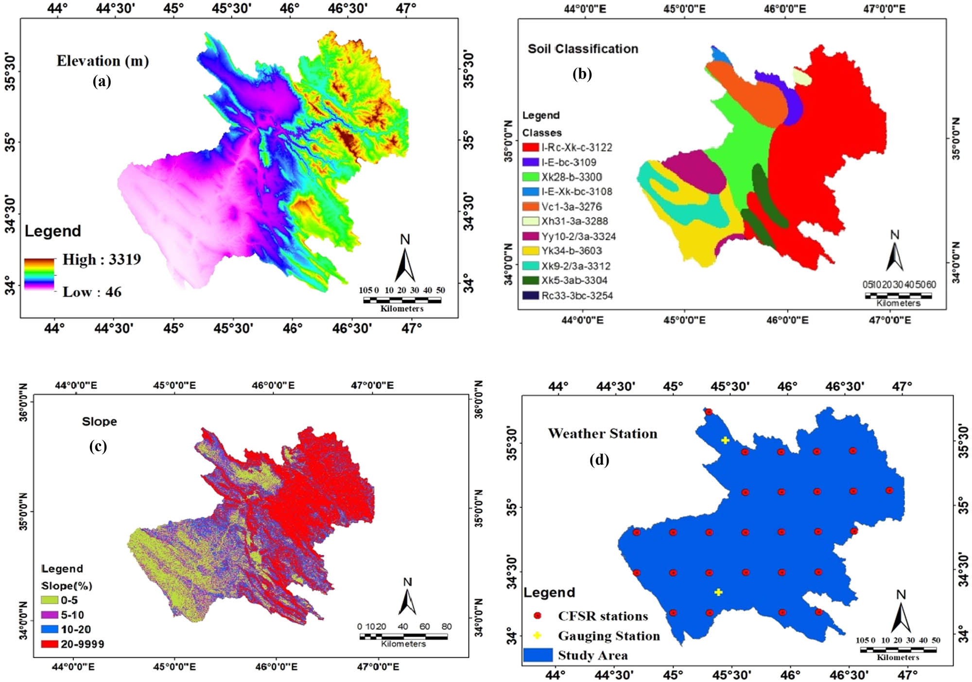
DRW information maps used in SWAT model. (a) Elevation, (b) soil classification, (c) slope, and (d) weather station.

4.2 Soil map

To understand how LULCC affects watershed’s hydrological components, soil data are important [2]. The soil type map for the present study was gained from Food and Agriculture Organization FAO-UNISCO soil, downloaded from the site https://www.fao.org/soils-portal/data in 2018. Eleven main soil sets were specified in the DRW, as shown in Table 1.

Table 1

Soil categories in the watershed of the Diyala River

No.	FAO soil code name	Code in arc SWAT	Hydrologic group	Soil type	Clay	Silt	Sand	Area (km²)
1	3108	I-E-Xk-bc-3108	D	Loam	24	43	34	140.17
2	3109	I-E-bc-3109	C	Loam	22	42	36	692.31
3	3122	I-Rc-Xk-c-3122	D	Loam	26	41	33	12142.78
4	3254	Rc33-3bc-3254	D	Loam	27	39	34	3.87
5	3276	Vc1-3a-3276	D	Clay	55	30	15	1983.51
6	3288	Xh31-3a-3288	D	Clay loam	34	34	31	189.05
7	3300	Xk28-b-3300	D	Clay loam	35	39	26	3135.82
8	3304	Xk5-3ab-3304	D	Clay loam	36	22	42	1110.97
9	3312	Xk9-2/3a-3312	D	Clay loam	31	32	36	1630.58
10	3324	Yy10-2/3a-3324	D	Clay	41	33	26	1570.99
11	3603	Yk34-b-3603	D	Loam	26	32	41	3052.53

Land use categories in the SWAT model are assigned four-letter codes. Therefore, LULC maps of the DRW were joined to SWAT land-use databases using these codes. The dominant characteristic of soil quality in the study area is Loam, Clay, and Clay Loam, and the hydrological group of the soil is classified according to group D. Figure 2b shows the classification of the soil maps in the DRW.

4.3 LULC

The LULC data from 2000 to 2020 were used to assess the effects of LULC variation on the hydrological components. For the present study, LULC was classified into five classes as indicated in Table 2 and, therefore, to study the impacts of LULCC in the study basin, each model has been well simulated each model separately.

Table 2

LULC category in the study area

No.	Definition in FAO	Definition in SWAT	SWAT code
1	Areas planted with herbaceous crops irrigated	Agricultural land generic	AGRL
2	Areas covered with bushes, open/closed shrubs, and combined with a small tree	Range brushland/shrubland	RNGB
3	Areas of rock or soil have foothills and valleys with a little diffusion vegetation for the entire year	Barren/wasteland areas	BARR
4	Areas that are covered with structures made by humans, such as paved roads, buildings, houses, towns, cities	Built-up area	URBN
5	Water-dominated areas all year round, such as rivers, lakes, and reservoirs	Water bodies	WATR

4.4 Slope

HRUs were classified into four categories of land slope (0–5, 5–10, 10–20, and above 20%), as shown in Figure 2c. HRUs were defined for the amounts of threshold as 0% for all datasets, soil, slope, and land use, then for each of the 33 sub-basins, HRUs were created.

4.5 Weather data

To construct the SWAT model for the studied watershed area, daily weather data are required, such as rainfall, minimum and maximum temperature, humidity relative, solar radiation, and wind speed. In SWAT, climate information can be provided from metrological station data in the study area or by data generated from the weather generation model (wgen) after checking the validity of the data measured by statistical analysis using Climate Forecast System Reanalysis (CFSR) of the global weather station. This method has been applied in many studies [23,26].

Therefore, to validate the results, we compared the precipitation from Khanaqen station with the precipitation from CFSR in a monthly time step from 1996 to 2014. During the monthly comparison, the values of R ² and Nash–Sutcliffe efficiency (NSE) were 0.77 and 0.76, respectively, which are within acceptable limits (Figure 3).

Figure 3

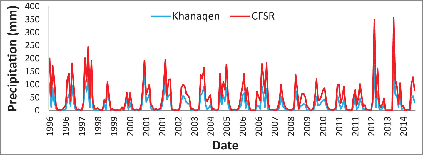
A monthly relation between CFSR and precipitation observed at Khanaqen meteorological station for the period 1996–2014.

4.6 Stream flow data

Daily stream flow data records for stream flow were gathered from gauging Hemren station (HS) and Derbendikhan station (DS) (Administration of HD and DD, Iraq, 2022, unpublished data) from 1996 to 2020. The average monthly data for flow were used for calibration and validation of the SWAT model.

5 Model set up

SWAT version 2012.10_5 was downloaded and its toolbar was integrated into GIS 10.5 to model hydrological systems. Based on the DEM collected, UTM 38 N coordinates were projected, and the drainage basin was divided into 33 sub-basins.

Sub-basins of the watershed were discretized using an automatic delineation DEM of (30 × 30) m. A definition of HRUs, LULC, slope, and soil class was executed by multiple classes of HRU using 0% for the threshold land use, slope, and soil to make it compatible with SWAT. There were construction 784 and 899 HRUs for the land uses for 2000 and 2020, respectively. After that, weather data were defined, and the model was with the default parameters with 4 years as a warm-up period. Then, SWAT simulation, sensitivity, calibration, and validation of the results were done. And finally, I ran the SWAT model for new parameters and obtained the results.

6 Criteria of calibration and validation in SWAT

Calibration is an operation to learn and amend input parameters to the observed value. At the same time, a validation compares model outputs with an independent dataset without altering parameters obtained during calibration [2].

The model of SWAT was calibrated and validated automatically using the sequential uncertainty fitting algorithm application (SUFI-2), which is embedded in the Uncertainty Procedures SWAT-CUP package [24].

To calibrate a sub-watershed or watershed, sensitive parameters must be identified to reduce the number of parameters that must be optimized before SWAT calibration and validation [4].

SUFI-2 determines the domain for any parameter, and then the Latin cube method is used to create many groups among calibration parameters; after that run, the model with each combination and the obtained outcomes are compared with the observed data to achieve the goal [24].

The model was validated and calibrated using SUFI-2 with monthly stream flow observed data, which was recorded in two gauging stations using LULC 2000: outlets of the DS and HS from 1996 to 2020. For the two outlets, the period from January 2000 to December 2013 was taken as calibration, and the period from January 2014 to December 2020 as a validation.

7 Performance of the model

The simulated and measured data were compared to evaluate the model’s performance. If the evaluation is within the range specified in Table 3, the performance is good; if it does not match, modify the input parameters until the best results are obtained.

Table 3

Performance ratings for recommended statistics for monthly time step [13,36]

Performance rating	Pbias (%)	R ²	NSE
Very good	Pbias < ± 10	0.8 ≤ R ² ≤ 1.0	0.75 < NSE ≤ 1.00
Good	±10 ≤ Pbias < ±15	0.7 ≤ R ² ≤ 0.75	0.65 < NSE ≤ 0.75
Satisfactory	±15 ≤ Pbias < ±25	0.5 ≤ R ² ≤ 0.6	0.50 < NSE ≤ 0.65
Unsatisfactory	Pbias > ±25	R ² < 0.5	NSE ≤ 0.50

In general, SWAT outputs were evaluated based on three statistical criteria [31]: coefficient of determination (R ²), NSE, and the percent bias (Pbias) as included in equations (6)–(8), respectively [23].

The coefficient of determination (R ²) shows the variance as a proportion between the observed and simulated values; it ranges between 0 and 1 and gives a reference of the relationship as a linear between the observed and simulated variables [32,33]. R ² is calculated as follows:
(6) R 2 = ∑ i = 1 n ( OB i − OM ) × ( SI i − SM ) ( ∑ i = 1 n ( OB i − OM ) 2 ) 0.5 × ( ∑ i = 1 n ( SI − SM ) 2 ) 0.5 2 .
NSE: The proportional values of the remaining variable, when compared to the variance of the observed data, range from (−∞ to 1) [34].

When the NSE value is closer to 1, this means there is good agreement between observed and simulated values. The formula of NSE is
(7) NSE = 1 − ∑ i = 1 n ( OB i − SI i ) 2 ∑ i = 1 n ( OB i − OM ) 2 .
Pbias is the amount of convergence and divergence between the measured and simulated values, and it is calculated as a percentage according to the following equation [15]:

(8) Pbias = ∑ i = 1 n ( OB i − SI i ) ∑ i = 1 n OB i × 100 ,

where OB_i is the measured values, OM is the average of measured values, SI_i is the simulated value, SM is the average of the simulated values, and n is the number of the observations to be considered.

In this study, based on the Pearson correlation matrix, linear correlations were evolved between hydrological components as dependent variables and LULC classes as independent variables, which have been applied in many studies [2,35].

8 Sensitivity assessment of the SWAT model

Initially, the DRW in the SWAT model has been carried out with initial parameters, and the outcomes have been displayed. Then, using SUFI-2 generated automatic calibration if we get to an acceptable match between observed and simulated values for the flow. The best parameters copy to Arc SWAT setup instead of the default parameters with the LULC 2000 map to find parameters with great sensitivity. Each iteration with 300 simulations was run, and the results of the analysis parameters are ranked with their increasing order of sensitivity.

9 Results and discussion

9.1 Discover of LULCC

Using supervised classification and satellite imagery Landsat, the LULCC for the DRW was observed and classified for two reference years, 2000 and 2020; also, five accounting classes were compared between the two years, as shown in Table 4.

Table 4

LULCC from 2000 to 2020 in the study area

No.	LULC	Area in km²		LULC change (2000–2020)
No.	LULC	LULC 2000	LULC 2020	LULC change (2000–2020)
1	Agricultural land generic	211	94	−117
2	Barren/wasteland	24,634	23,473	−1,161
3	Range brush/shrubland	453	517	64
4	Built up area	178	1345	1,167
5	Water bodies	176	223	47
	Total	25,652	25,652

Table 4 presents information about the area of LULC, while Figure 4 compares qualitative LULCC in 2000 and 2020 in the study area.

Figure 4

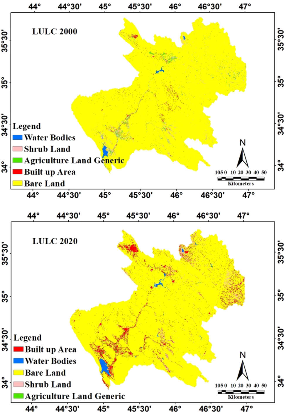
Spatial distribution of LULC in DRW in 2000 and 2020.

Fast growth in the built-up class is observed in an extra amount of 1,167 km² from 2000 to 2020. Population growth, settlement (built-up) area expansion, and social and economic factors are responsible for the increase [4,5]. The shrubland area has also increased by 64 km²; however, the bare land was reduced from 24,634 km² in 2000 to 23,473 km² in 2020 due to increasing settlement area. The water bodies were a little increased from 176 km² in 2000 to 223 km² in 2020 due to an increase in the reservoirs of DD and HD, which occurred due to a large amount in average annual precipitation in 2019 with amounts of 480 mm (Administration of HD and DD, Iraq, 2022, unpublished data). Agricultural lands decreased by 117 km² during the same period despite the increase in the rain due to the lack of economic feasibility in agriculture and people resorting to imported foods that are cheaper in addition to fluctuating amounts of precipitation from year to year.

In contrast, the wasteland areas decreased by 1,171 km² due to the tendency of people to increase settlement areas because of maximized population and urban expansion.

Changes occurred in all categories of LULC. However, the most significant changes were observed in the built-up (urbanization) areas. LULCC between 2000 and 2020 in various sub-basin areas was calculated (Figure 5). They displayed how the built-up, agricultural land generic, barren land, shrubland, and water bodies have changed spatially in various sub-basins of the DRW.

Figure 5

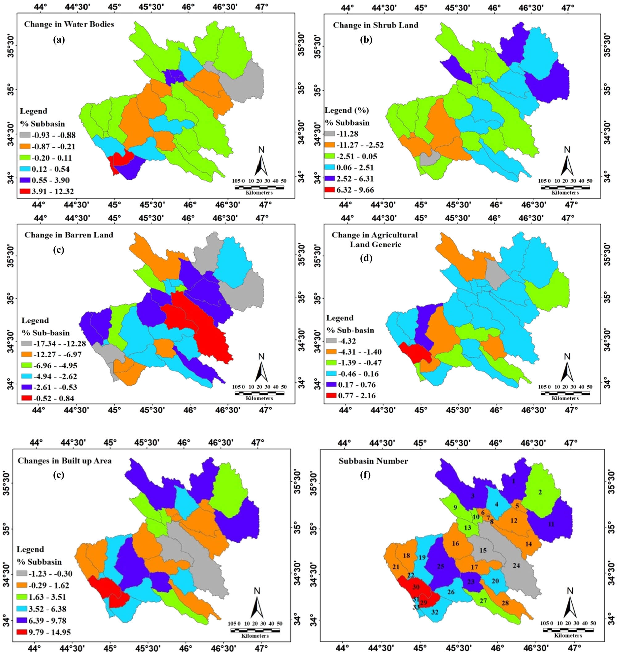
LULU changes in sub-basins (a) water bodies, (b) shrub lands, (c) barren land, (d) agricultural land generic, (e) built-up area, and (f) sub-basin number in the Diyala River basin (2000–2020).

In the water bodies area, the basin increased from 0.69% in 2000 to 0.87% in 2020 which increases in sub-basin 31(12.3%) and sub-basin 33(8.3%) and reduces in sub-basin 11(−0.93%) according to Figure 5a.

Figure 5b shows the change in shrub lands in sub-basins from 9.66% in sub-basin 8 to −11.28% in sub-basin 29. The quantity of barren land in the basin decreased by – 4.5%, while the sub-basin area was found in sub-basin 8 (−17.3%), sub-basin 1 (−15.17%), sub-basin 30 (−13.38%), and sub-basin 15 (0.84%), as illustrated in Figure 5c. Similarly, at the basin, the agricultural land generic has reduced from 0.82% in 2000 to 0.37% in 2020, whereas at the sub-basin level, the higher value in sub-basin 30 (2.1%) and the minimum value in sub-basin 4 (−4.32%), as shown in Figure 5d.

In Figure 5e and at the level of the sub-basin area, the built-up changes are between 14.9 and 1.2%, whereas at the basin level, 5.2% over the same period. The higher increase in urban areas was specified in sub-basin 29 (14.9%), sub-basin 30 (14.6%), and sub-basin 25 (9.8%).

9.2 Accuracy of the land use classification

From Tables 5 and 6 and according to this study, there are 158 and 143 random reference points for the years 2000 and 2020 that were carried out to assist the accuracy of LULCC, which is spread over the entire study area.

Table 5

Confusion matrix of LULC in 2000

LULC	WB	BU	BS	SL	AG	Total	User’s (%)
WB	61	0	2	1	0	64	95.31
BU	1	30	1	0	0	32	93.75
BS	0	0	16	1	1	18	88.89
SL	1	0	0	21	2	24	87.5
AG	0	0	2	1	17	20	85
Total	63	30	21	24	20	158	OA = 91.77
Producer’s (%)	96.83	100	76.19	87.5	85		ka = 88.97

WB: water body; BU: built up; BS: bare soil; SL: shrub land; AG: agricultural land generic.

Table 6

Confusion matrix of LULC in 2020

LULC	WB	BU	BS	SL	AG	Total	User’s (%)
WB	57	0	1	0	0	58	98.28
BU	0	22	1	0	0	23	95.65
BS	0	0	17	1	0	18	94.44
SL	0	0	0	23	1	24	95.44
AG	0	0	0	0	20	20	100
Total	27	22	19	24	21	143	OA = 97.2
Producer’s (%)	100	100	89.47	95.83	95.24		ka = 96.26

WB: water body; BU: built up; BS: bare soil; SL: shrub land; AG: agricultural land generic.

For ground-truthing, imagery of Google Earth in 2000 and 2020 was used. For the two Landsat images, the OA and ka were equal to 91.77 and 88.97% for 2000, and 97.2 and 96.26% for 2020, respectively. The results obtained comply with the minimum standard accuracy of 85% for the classification of LULC [2]. From the results, it can be noticed that most pixels have been correctly classified. The results of the obtained ka values are considered very well when compared with the permissible values, which are between 0.81 and 1 [3,5].

By technique of intersecting LULC classes from 2000 to 2020, an LULC transformation matrix was improved for the LULCC from 2000 to 2020 by overlaying the classified LULC map for the year 2000 with the classified LULC map in 2020 and specifying the areas where the LULCC does not change from one class to another [7].

9.3 Sensitivity analysis

At first, 20 parameters were chosen for the sensitivity analysis according to previous studies. After conducting a series of simulations, the most sensitive of these parameters was chosen. Table 7 shows that the most sensitive parameter values were taken through the calibration process.

Table 7

Sensitivity parameters for the streamflow in the study area

Rank	Parameter name	Description	Fitted value	Initial range
Rank	Parameter name	Description	Fitted value	min	max
1	R__CN2.mgt	SCS runoff curve number factor	−0.054	−0.5	0.5
2	R__SOL_AWC(. ).sol	Available water capacity of the soil layer	0.1	−0.3	0.5
3	V__ALPHA_BF.gw	The alpha factor for base flow	0.71	0	1
4	V__GW_DELAY.gw	Delay of groundwater	240	30	450
5	R__ESCO.hru	The factor of soil evaporation	0.64	0	1
6	V_PCPD(. ).wgn	The mean number of rainy days per month	13.8	0	31
7	R__GW_REVAP.gw	Groundwater “revap” coefficient	0.025	0.02	0.2
8	R__CH_K2.rte	Effective hydraulic conductivity in main channel alluvium	117.5	5	130
9	R__REVAPMN.gw	Threshold depth of water in the shallow aquifer for “revap” to occur (mm)	65.58	0	100
10	R__OV_N.hru	Manning’s “n” value for overland flow	0.1	−0.3	0.3
11	R__SOL_K(. ).sol	Saturated hydraulic conductivity	0.24	−0.1	0.35
12	R__CH_N2.rte	Manning’s “n” value for the main channel	0.21	0	0.3
13	R__SLSUBBSN.hru	Average slope length	0.02	0	0.2
14	R__SMFMX.bsn	Maximum melt rate for snow during the year (occurs on the summer solstice)	18	0	20
15	V__GWQMN.gw	Threshold depth of water in the shallow aquifer required for return flow to occur (mm)	1	65.3	100

9.4 Calibration and validation model

A time series was plotted between simulated and observed values of stream flow as a monthly flow for the calibration period (January 2000 to December 2013) and validation period (January 2014 to December 2020) for the two gauging stations in HD and DD as shown in Figures 6 and 7, respectively. The statistic values for the model’s performance for the R ², NSE, and Pbias are shown in Table 8. According to Table 8, the model’s performance is good.

Figure 6

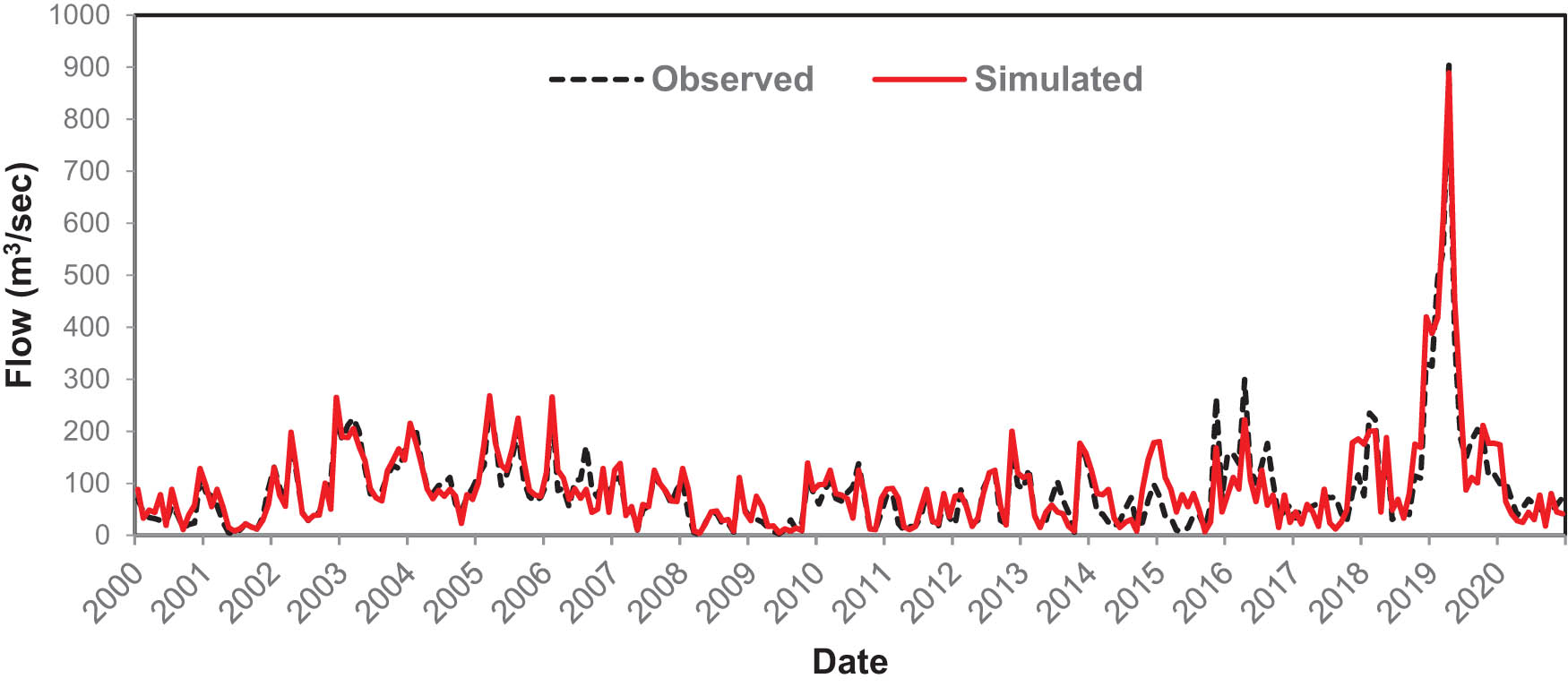
Calibration and validation of the SWAT model in HD from 2000 to 2020.

Figure 7

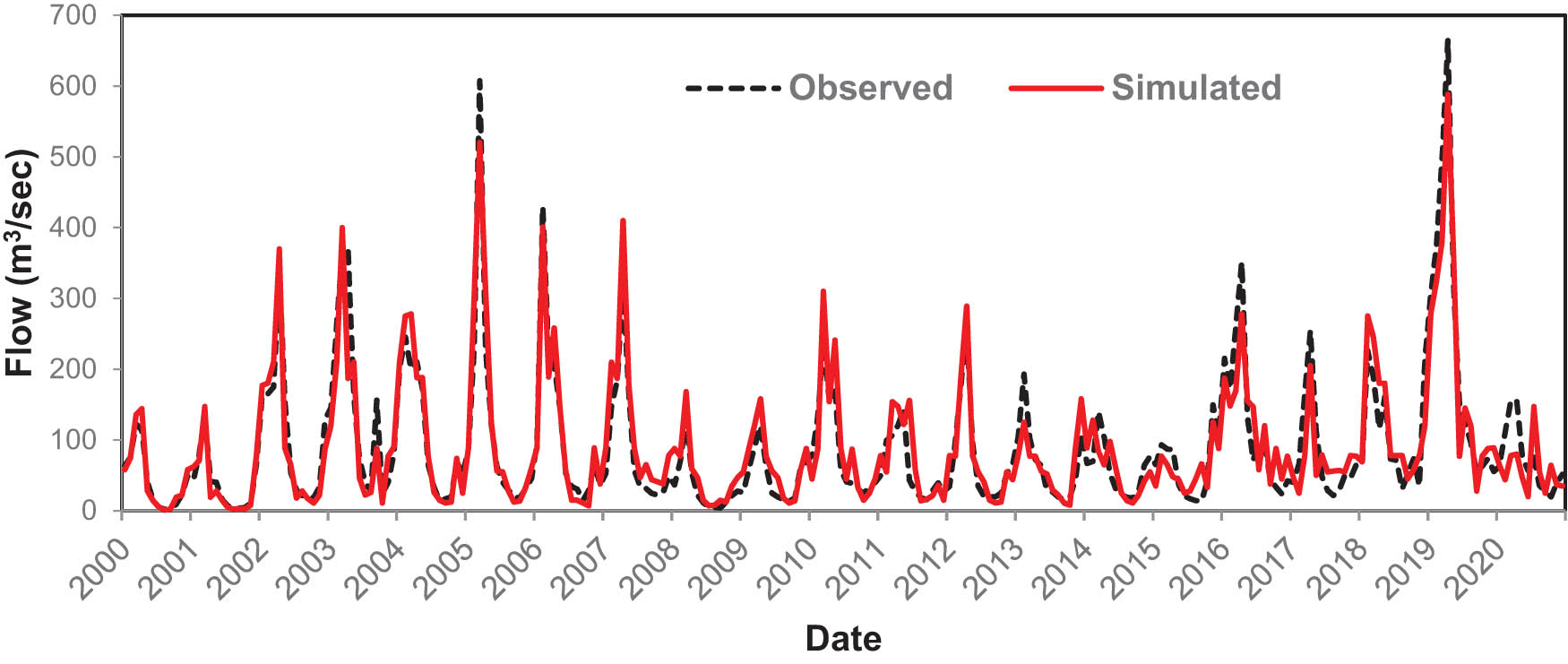
Calibration and validation of the SWAT model in DD from 2000 to 2020.

Table 8

Model evaluation criteria for streamflow modeling throughout calibration and validation time

Statistical indices	Gauging station
	HD		DD
	Calibration	Validation	Calibration	Validation
R ²	0.85	0.84	0.88	0.85
NSE	0.87	0.85	0.87	0.85
Pbias (%)	4.2	5.8	+6.8	−4.1
R-factor	0.54	0.38	0.48	0.38
P-factor	0.72	0.74	0.74	0.71

9.5 Impact of LULCC on water resources

9.5.1 Basin-scale

Table 9 shows that the mean yearly basin (2000–2020) values of the WYLD, LATQ, SURQ, ET, and PER were simulated from every LULC map. A baseline scenario of the 2000 LULC map is used to determine the effect of LULCC on hydrology. According to the map of LULC 2000, the mean yearly WYLD on the basin is 4.77 mm less than the 2020 LULC map compared to the simulation period (2000–2020).

Table 9

Summary of LULCC and average annual water balance for the DRW from 2000 to 2020, using 2000 and 2020 LULC maps

Time period	AG (%)	BL (%)	WB (%)	SL (%)	BU (%)	SURQ (mm)	WYLD (mm)	PER (mm)	LATQ (mm)	ET (mm)
2000	0.82	96.0	0.67	1.77	0.69	107.82	113.65	7.49	4.52	202.9
2020	0.37	91.5	0.87	2.02	5.2	112.67	118.42	7.21	4.42	209.8
2000–2020	−0.45	−4.5	0.2	0.25	4.51	4.85	4.77	−0.28	−0.10	6.9

Also, the mean yearly SURQ for the LULC 2020 was 4.85 mm, which was bigger than that of the map of LULC 2000, which grew by 4.3%. In contrast, the mean annual PER for the LULC 2000 map was 0.28 mm, lower than the 2020 LULC map. In the basin, the expansion in built-up lands generally leads to decreasing percolation [4]. Similarly, LATQ decreased by a very small amount of 0.1 mm from 2000 to 2020 LULC maps.

ET decreased from LULC map 2000 to LULC map 2020 by 6.9 mm, associated with increasing water bodies. Typically, an increase in SURQ and a decrease in PER in over basin were connected with the increase in the urban area. At the sub-basin level, the variations in hydrological components are higher than the model precision concerning LULCC.

9.5.2 At the sub-basin scales

Using correlation analysis, the spatial effect of LULCC was investigated between proportional LULCC and change in components of hydrological gained through variation in simulation using LULC maps in 2000 and 2020 [5,35].

The relationship between LULC and hydrological components (at the sub-basin level) can be clarified using the correlation coefficient (R) in the correlation matrix shown in Table 10. Also, it references the kind of transformation among classes of LULC in various sub-basins of DRW. There is no doubt that LULCC is affecting hydrological components at a sub-watershed level in a significant way.

Table 10

Correlation coefficient was calculated between changes in the percentage of LULC and changes in the hydrological components between 2000 and 2020 in the DRW

	URBN	WATR	RNGB	AGRL	BARR	ET	PERC	SURQ	WYLD	LAT_Q
URBN	1.00
WATR	0.08	1.00
RNGB	−0.42	−0.20	1.00
AGRL	−0.20	−0.03	0.27	1.00
BARR	−0.56	−0.50	−0.28	−0.22	1.00
ET	0.13	0.77	−0.02	0.02	−0.56	1.00
PERC	−0.26	−0.11	0.69	0.24	−0.25	0.15	1.00
SURQ	0.85	0.11	−0.37	−0.25	−0.47	0.06	−0.36	1.00
WYLD	0.66	0.04	−0.27	−0.34	−0.32	0.08	−0.40	0.81	1.00
LAT_Q	−0.31	−0.11	0.16	−0.14	0.24	0.02	−0.07	−0.30	0.31	1.00

A minus correlation (R = −0.56) between the built-up area and barren area shows that decreasing barren area drives revenue in the built-up. Similarly, urban area correlated with shrubland area (R = −0.42) and agricultural area (R = −0.2). That means the sub-basin’s agricultural, barren, and shrub lands decreased because of built-up expansion. Also, the hydrological components for the correlation matrix detect the relationship between LULCC in the same catchment areas.

By minimizing the analysis to a sub-basin level, it is possible to get sufficient learning of the main hydrological processes in the basin [4].

Figure 8 illustrates changes in the sub-basin for the WYLD, SURQ, LATQ, PER, and ET in the LULC from 2000 to 2020. The expansion in built-up areas had a plus correlation with WYLD (R = 0.66), SURQ (R = 0.85), and ET (R = 0.13); on the contrary, a negative relation with PER (R = −0.26) and LATQ (R = −0.31). Sub-basin analysis provides high clarity for the hydrological processes in the basin, as shown in Figure 8a.

Figure 8

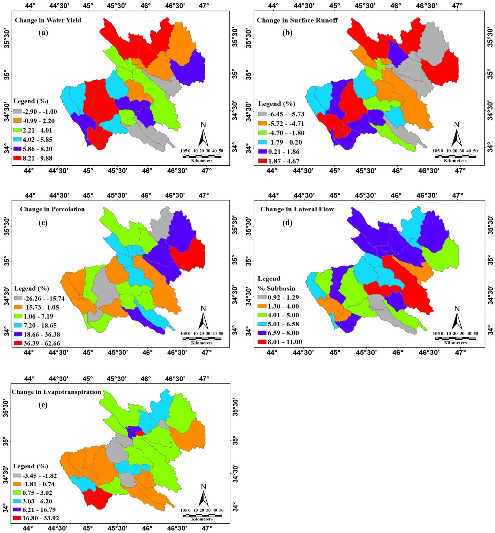
Hydrological components at the sub-basin scale from 2000 to 2020: (a) water yield, (b) SURQ, (c) percolation, (d) lateral flow, and (e) evapotranspiration.

The change in average yearly SURQ differs from −6% in sub-basin 28 to 4.67% in sub-basin 29 (14.95% increase in built-up areas), as described in Figure 8b.

Expansion in the built-up area in sub-basin 29 (14.95%), sub-basin 30 (14.64%), and sub-basin 25 (3.85%) illustrated an increase in SURQ by 4.67, 4.25, and 3.85% for sub-basins 29, 30, and 25, respectively. The high correlation between the built-up area and SURQ shows the growth in the built-up area concerning changes in SURQ. Similarly, expansion in the sub-basins built-up area leads to an increase in WYLD. The mean yearly changes in WYLD were between −2.9% in sub-basin 14 and 9.88% in sub-basin 3 – the increase in WYLD links with increasing SURQ and, subsequently, with expansion in the built-up area.

In sub-basin 29, with expansion in built-up area by 14.95% connected with increase in SURQ by 4.67% and WYLD by 8.67%. Similarly, sub-basin 30 (14.95%) expansion in built-up areas and sub-basin 25 expansion in built-up area (14.64%) shows an increase in SURQ 4.25 and 3.85%, leading to an increase in WYLD 7.25 and 8.85%. Generally, there was a high correlation between increases in an urban area and an increase in WYLD [4].

The water that attains the major river channel through the soil profile is called the LATQ. It has a significant impact on the soils at lower depths, which have impermeable layers. The LATQ varies from 1.29% in sub-basin 23 to 17% in sub-basin 11. Figure 8c shows the PER changes from −26.26% in sub-basin 29 (which has a higher increase in a built-up area of 14.9%) to 62.66% in sub-basin 11.

The high lateral flow is appreciated in sub-basin 17 (11%) and sub-basin 24 (9.02%). Figure 8d offers a relation between LATQ and changes in built-up areas in the basin.

ET includes transpiration and evaporation from vegetation and soil [4]. The difference between precipitation and ET is that water is useful for management and human use. ET changes from −3.45% in sub-basin 5 to 33.92% in sub-basin 8, as shown in Figure 8e.

Figure 8e shows a high correlation of coefficient (R = 0.77) between water bodies and ET. In the sub-basin with high built-up, a marginal decline in ET was observed.

For example, increase in water bodies in sub-basin 33, sub-basin 8, and sub-basin 29 had just 8.22, 3.57, and 7.13% growth, which illustrated an increase in ET by 33.92, 33.39, and 28.16%, respectively.

10 Conclusions

The SWAT model can be used to find the impact of LULCC on the ET, SURQ, WYLD, PER, and LATQ in DRW, which witnessed several changes from 2000 to 2020.

The summarized conclusions are as follows:

The weather data from the CFSR are considered reliable to represent the weather data inputs into the SWAT model.
The resolution of (30 × 30) m LULC map for Landsat satellite images is suitable for showing changes in LULC at the supervised classification, as this resolution has been used in many studies [2,35].
The possibility of using the SWAT model for hydrological representation in DRW is without problems, with calibration and verification of the results using SUFI.
Despite the increase in the built-up area from 0.96% in the year 2000 to 5.2% in the year 2020, as well as the decrease in barren land from 96 to 91.5%, the impacts on the level of hydrological components are small about the basin.
The increase in urban expansion and the decrease in wastelands were considered the two largest variables at the basin level during the study period. Therefore, it was studied in more detail at the level of the sub-basins. Using statistical correlation analysis, it was found that the increase in urban expansion has a positive relationship with the increase in SURQ and WYLD, as the increasing SURQ has negative effects on the DRW by increasing environmental problems by generating erosion.
ET is slightly affected by urban expansion, but it has a strong positive relationship with the increase in water bodies and a negative with barren lands.
There is a negative relationship between the decline of wastelands and urban expansion, which indicates that urban expansion tends more to desert lands, which leads to their decline.

Therefore, this study may be provided to project future strategies for managing water resources in DRW.

We strongly recommend that more future research to be carried out on the River basin to investigate the effect of LULCC on the relationship of change in the runoff with flooding and hydrological response. Also, the local authorities should participate in setting up more points for climate information and that it should be distributed sufficiently and regularly in the region, where poor data obtained lead to the program’s implementation being an unacceptable and unreliable result.

tel: +964 07702690516

Funding information: The authors state no funding involved.
Conflict of interest: The authors state no conflict of interest.
Competing interest: The authors state no competing interest.
Data availability statement: Most datasets generated and analyzed in this study are in this submitted manuscript. The other datasets are available on reasonable request from the corresponding author with the attached information.

References

[1] Osei MA, Amekudzi LK, Wemegah DD, Preko K, Gyawu ES, Obiri-Danso K. The impact of climate and land-use changes on the hydrological processes of Owabi catchment from SWAT analysis. J Hydrol: Reg Stud. 2019;25:100620.10.1016/j.ejrh.2019.100620Search in Google Scholar

[2] Kenea U, Adeba D, Regasa MS, Nones M. Hydrological responses to land use land cover changes in the fincha’a watershed. Ethiopia Land. 2021;10(9):916.10.3390/land10090916Search in Google Scholar

[3] Aga HT. Effect of land cover change on water balance components in Gilgel Abay catchment using swat model. Netherlands: University of Twente; 2019.Search in Google Scholar

[4] Samal DR, Gedam S. Assessing the impacts of land use and land cover change on water resources in the Upper Bhima river basin, India. Environ Chall. 2021;5:100251.10.1016/j.envc.2021.100251Search in Google Scholar

[5] Gyamfi C, Ndambuki JM, Salim RW. Hydrological responses to land use/cover changes in the Olifants Basin, South Africa. Water. 2016;8(12):588.10.3390/w8120588Search in Google Scholar

[6] Worku T, Khare D, Tripathi S. Modeling runoff–sediment response to land use/land cover changes using integrated GIS and SWAT model in the Beressa watershed. Environ Earth Sci. 2017;76:1–14.10.1007/s12665-017-6883-3Search in Google Scholar

[7] Ganapathi H, Phukan M, Vasudevan P, Palmate SS. Assessing the impact of land use and land cover changes on the water balances in an urbanized peninsular region of India. In Current directions in water scarcity research. Netherlands: Elsevier; 2022. p. 225–42.10.1016/B978-0-323-91910-4.00014-5Search in Google Scholar

[8] Larbi I, Obuobie E, Verhoef A, Julich S, Feger KH, Bossa AY, et al. Water balance components estimation under scenarios of land cover change in the Vea catchment, West Africa. Hydrol Sci J. 2020;65(13):2196–209.10.1080/02626667.2020.1802467Search in Google Scholar

[9] Da Silva VDP, Silva MT, Souza EPD. Influence of land use change on sediment yield: a case study of the sub-middle of the São Francisco river basin. Eng Agríc. 2016;36:1005–15.10.1590/1809-4430-eng.agric.v36n6p1005-1015/2016Search in Google Scholar

[10] dos Santos JYG, Montenegro SMGL, Silva RM, Santos CAG, Quinn NW, Dantas APX, et al. Modeling the impacts of future LULC and climate change on runoff and sediment yield in a strategic basin in the Caatinga/Atlantic forest ecotone of Brazil. Catena. 2021;203:105308.10.1016/j.catena.2021.105308Search in Google Scholar

[11] Huang TC, Lo KFA. Effects of land use change on sediment and water yields in Yang Ming Shan National Park, Taiwan. Environments. 2015;2(1):32–42.10.3390/environments2010032Search in Google Scholar

[12] Abu-Zreig M, Hani LB. Assessment of the SWAT model in simulating watersheds in arid regions: Case study of the Yarmouk River Basin (Jordan). Open Geosci. 2021;13(1):377–89.10.1515/geo-2020-0238Search in Google Scholar

[13] Birhanu SY, Moges MA, Sinshaw BG, Tefera AK, Atinkut HB, Fenta HM, et al. Hydrological modeling, impact of land-use and land-cover change on hydrological process and sediment yield; case study in Jedeb and Chemoga watersheds. Energy Nexus. 2022;5:100051.10.1016/j.nexus.2022.100051Search in Google Scholar

[14] Mengistu AG, van Rensburg LD, Woyessa YE. Techniques for calibration and validation of SWAT model in data scarce arid and semi-arid catchments in South Africa. J Hydrol: Reg Stud. 2019;25:100621.10.1016/j.ejrh.2019.100621Search in Google Scholar

[15] Awotwi A, Anornu GK, Quaye-Ballard JA, Annor T, Forkuo EK, Harris E, et al. Water balance responses to land-use/land-cover changes in the Pra River Basin of Ghana, 1986–2025. Catena. 2019;182:104129.10.1016/j.catena.2019.104129Search in Google Scholar

[16] Juma LA, Nkongolo NV, Raude JM, Kiai C. Assessment of hydrological water balance in Lower Nzoia Sub-catchment using SWAT-model: towards improved water governace in Kenya. Heliyon. 2022;8(7):e09799.10.1016/j.heliyon.2022.e09799Search in Google Scholar PubMed PubMed Central

[17] Nyatuame M, Amekudzi LK, Agodzo SK. Assessing the land use/land cover and climate change impact on water balance on Tordzie watershed. Remote Sens Appl: Soc Environ. 2020;20:100381.10.1016/j.rsase.2020.100381Search in Google Scholar

[18] Kouchi DH, Esmaili K, Faridhosseini A, Sanaeinejad SH, Khalili D, Abbaspour KC. Sensitivity of calibrated parameters and water resource estimates on different objective functions and optimization algorithms. Water. 2017;9(6):384.10.3390/w9060384Search in Google Scholar

[19] Wagner P, Kumar S, Schneider K. An assessment of land use change impacts on the water resources of the Mula and Mutha Rivers catchment upstream of Pune, India. Hydrol Earth Syst Sci. 2013;17(6):2233–46.10.5194/hess-17-2233-2013Search in Google Scholar

[20] Manhi HK, Al-Kubaisi QYS. Estimation annual runoff of Galal Badra transboundary Watershed using Arc Swat model, Wasit, East of Iraq. Iraqi Geol J. 2021;54:69–81.10.46717/igj.54.1D.6Ms-2021-04-26Search in Google Scholar

[21] Abbaspour KC, Rouholahnejad E, Vaghefi S, Srinivasan R, Yang H, Kløve B. A continental-scale hydrology and water quality model for Europe: Calibration and uncertainty of a high-resolution large-scale SWAT model. J Hydrol. 2015;524:733–52.10.1016/j.jhydrol.2015.03.027Search in Google Scholar

[22] Risal A, Parajuli PB, Dash P, Ouyang Y, Linhoss A. Sensitivity of hydrology and water quality to variation in land use and land cover data. Agric Water Manag. 2020;241:106366.10.1016/j.agwat.2020.106366Search in Google Scholar

[23] Khayyun TS, Alwan IA, Hayder AM. Hydrological model for Hemren dam reservoir catchment area at the middle River Diyala reach in Iraq using ArcSWAT model. Appl Water Sci. 2019;9:1–15.10.1007/s13201-019-1010-0Search in Google Scholar

[24] Abbas N, Wasimi SA, Al-Ansari N. Impacts of climate change on water resources in Diyala River Basin, Iraq. J Civ Eng Archit. 2016;10(9):1059–74.10.17265/1934-7359/2016.09.009Search in Google Scholar

[25] Al-Khafaji MS, Al-Chalabi RD. Impact of climate change on the spatiotemporal distribution of stream flow and sediment yield of Darbandikhan watershed, Iraq. Eng Technol J. 2020;38(2 Part A):265–76.10.30684/etj.v38i2A.156Search in Google Scholar

[26] Naqi NM, Al-Jiboori MH, Al-Madhhachi A-ST. Statistical analysis of extreme weather events in the Diyala River basin, Iraq. J Water Clim Change. 2021;12(8):3770–85.10.2166/wcc.2021.217Search in Google Scholar

[27] Kareem HH, Alkatib AA. Future short-term estimation of flowrate of the Euphrates river catchment located in Al-Najaf Governorate, Iraq through using weather data and statistical downscaling model. Open Eng. 2022;12(1):129–41.10.1515/eng-2022-0027Search in Google Scholar

[28] Tadesse W, Whitaker S, Crosson W, Wilson C. Assessing the impact of land-use land-cover change on stream water and sediment yields at a watershed level using SWAT. Open J Mod Hydrol. 2015;5(3):68–85.10.4236/ojmh.2015.53007Search in Google Scholar

[29] Devia GK, Ganasri BP, Dwarakish GS. A review on hydrological models. Aquat Procedia. 2015;4:1001–7.10.1016/j.aqpro.2015.02.126Search in Google Scholar

[30] Gu X, Yang G, He X, Zhao L, Li X, Li P, et al. Hydrological process simulation in Manas River Basin using CMADS. Open Geosci. 2020;12(1):946–57.10.1515/geo-2020-0127Search in Google Scholar

[31] Akoko G, Le TH, Gomi T, Kato T. A review of SWAT model application in Africa. Water. 2021;13(9):1313.10.3390/w13091313Search in Google Scholar

[32] Megersa L, Tamene D, Koriche S. Impacts of land use land cover change on sediment yield and stream flow: A case of finchaa hydropower reservoir, Ethiopia. UK. Int J Sci Technol. 2017;6:763–81.Search in Google Scholar

[33] Al-Ansari N, Abdellatif M, Ali S, Knutsson S. Long term effect of climate change on rainfall in northwest Iraq. Open Eng. 2014;4(3):250–63.10.2478/s13531-013-0151-4Search in Google Scholar

[34] Saputra AWW, Zakaria NA, Weng CN. Changes in land use in the Lombok River Basin and their impacts on river basin management sustainability. In IOP Conference Series: Earth and Environmental Science. IOP Publishing; 2020.Search in Google Scholar

[35] Serur AB, Adi KA. Multi-site calibration of hydrological model and the response of water balance components to land use land cover change in a rift valley Lake Basin in Ethiopia. Sci Afr. 2022;15:e01093.10.1016/j.sciaf.2022.e01093Search in Google Scholar

[36] Nie W, Yuan Y, Kepner W, Nash MS, Jackson M, Erickson C. Assessing impacts of Landuse and Landcover changes on hydrology for the upper San Pedro watershed. J Hydrol. 2011;407(1–4):105–14.10.1016/j.jhydrol.2011.07.012Search in Google Scholar

Received: 2023-03-31

Revised: 2023-05-01

Accepted: 2023-05-06

Published Online: 2023-10-10

This work is licensed under the Creative Commons Attribution 4.0 International License.

Articles in the same Issue

https://doi.org/10.1515/eng-2022-0456

Keywords for this article

Arc SWAT model; Diyala River; hydrological model; LULC changes

Creative Commons

BY 4.0