Dislocated time sequences – deep neural network for broken bearing diagnosis

Pramudyana Agus Harlianto; Teguh Bharata Adji; Noor Akhmad Setiawan

doi:10.1515/eng-2022-0402

Artikel Open Access

Dislocated time sequences – deep neural network for broken bearing diagnosis

Pramudyana Agus Harlianto , Teguh Bharata Adji und Noor Akhmad Setiawan

Veröffentlicht/Copyright: 31. März 2023

Veröffentlicht von

Veröffentlichen auch Sie bei De Gruyter Brill

Manuskript einreichen Informationen für Autor*innen

Aus der Zeitschrift Open Engineering Band 13 Heft 1

Abstract

One of the serious components to be maintained in rotating machinery including induction motors is bearings. Broken bearing diagnosis is a vital activity in maintaining electrical machines. Researchers have explored the use of machine learning for diagnostic purposes, both shallow and deep architecture. This study experimentally explores the progress of dislocated time sequences–deep neural network (DTS–DNN) used to improve multi-class broken bearing diagnosis by using public data from Case Western Reserve University. Deep architectures can be utilized with the purpose of simplifying or avoiding any traditional feature extraction process. DNN is utilized for avoiding the pooling operation in Convolution neural network that could remove important information. The obtained results were compared with the present techniques. The examination resulted in 99.42% average accuracy which is higher than the present techniques.

Keywords: dislocated time sequences; deep neural network; broken bearing diagnosis; accuracy; multi-class

1 Introduction

In many cases, electric motors are the equipment that plays a major role in making the production system function. Maintenance activities will be expensive because they can involve unprepared stoppage and harm to the production process due to equipment damage, such as induction motor damage [1].

Fault diagnosis is an important activity in maintaining electrical machines. Fault diagnosis has the capability to decrease repair costs and avoid accidents [2,3]. Capability to identify and diagnose the faults is the greatest technology in condition-based maintenance systems, especially for rotating machines [4]. One important component in an electric engine is a bearing.

Bearings are considered a vital element in an electric motor or engine [5]. Broken bearings are the foremost cause of engine damage, so diagnosing of broken bearing is vital [6,7]. Diagnosing broken bearing is able to be performed in the old-style technique or utilizing present methods by using machine learning (ML) or deep learning approaches.

The technique of diagnosing broken bearings has made utilization of ML approach. Selection of proper algorithms and influencing input variables are very important to analyze broken conditions [8,9]. ML methods have the capability of answering the problem of remote control, diagnosing the broken part, and non-linearity [10]. Some of the approaches used to be combined with ML for feature extraction are analysis of statistic [4,11], transformation signal by using Fourier method [12], time frequency transformation (wavelet) [13,14], empirical mode decomposition (EMD) [8,15,16], representation of sparse [17], and dimensionality reduction (DR) [18]. ML methods have been utilized for diagnosing purposes such as support vector machine (SVM) [19,20], Artificial neural networks [21], models of hidden Markov [22], random forest (RF) approach [4], and using method of k-nearest neighbor [23,24]. These approaches are habitually considered in approaches with un-deep architectures or shallow configurations. These shallow configuration approaches have limitations when they come to current fault diagnosis problems. The limitations include overfitting, un-convergence training, poor performance, and difficulty with nonlinear and complex functions [24].

Several approaches have been assessed by researchers for improving limitations of conventional approaches. The approach of deep learning has been broadly utilized for diagnosing broken bearing. For example, the bearing broken at rolling elements and planetary gearboxes were diagnosed by utilizing Deep artificial neural configuration [25]. Convolution artificial neural configuration/network (CNN) is utilized to obtain the determining features to diagnose the broken condition of rotating machines [24,26,27]. Dislocated time sequences CNN (DTS–CNN) was utilized to advance CNN configuration, constructed to handle the features signals of mechanics [28]. Deep statistical analysis was used for vibration signals feature learning generated from a rotating machine [29]. The algorithm of artificial fish swam is utilized for optimizing the determining parameters of the deep autoencoder [30]. The method of deep belief networks (DBNs) with adaptive learning by using packet of double-three complex wavelets (DTCWPT) were assessed for broken bearing diagnosis by using data from Case Western Reserve University (CWRU) [31].

For diagnosing broken bearings, deep learning still requires a transformation process to transform raw signal time domain to another domain such as frequency or wavelet. DBN with DTCWPT still requires time frequency signal input on diagnosing broken bearing from CWRU. The best accuracy achieved for 16 classes bearing faults was 95.2% [31]. DBN, CNN, and Sparse auto encoder successfully achieved accuracy of 96.87, 99.125, and 100% for 6 classes broken bearing from CWRU. Three of these methods transformed raw signal into wavelet scalogram [24]. DTS–CNN successfully diagnoses broken bearings from raw signal time domains from private datasets. The accuracy achieved by DTS–CNN is 96.32% [28].

The combined DTS–CNN approach allows CNN to excerpt the features that are continuously fed to SoftMax for classification. The result of excerpting the feature is that there is the potential for duplication (redundancy) and potential for containing useless information. It is certain that this condition will have an impact on the classifier’s performance. The other aspect that influences classifiers performance include how many input features are used [28]. The significant mistake in CNN could be caused by a pooling operation. The pooling operation also works as a destroyer (disaster) [32]. There is a possibility that location information was removed by pooling layers [33].

The state of the art (currently available approach) of broken bearing diagnosis is summarized in Table 1.

Table 1

Currently available approach of broken bearing diagnosis

Current approach	Limitation
Shallow configuration of ML such as neural network, SVM	Shall be combined with feature extraction, for example, analysis of statistics, Fourier transformation, transformation of wavelet, EMDs, representation of sparse, and DR. Shallow configuration could not directly utilize time domain signal for diagnosing broken bearing.
Shallow configuration of ML such as neural network, SVM	There are limitations such as overfitting, un-convergence training, poor performance, difficulty with nonlinear, and complex functions.
DBN	Requires time frequency signal as input (wavelet). The performance (accuracy) is 95.2%.
(DTS–CNN)	There is a significant mistake in CNN that could be caused by a pooling operation. The performance (accuracy) achieved is 96.32%.
(DTS–CNN)	There is a possibility to improve this accuracy utilizing simpler and faster deep learning configuration (DNN).

The problems to be solved in this study are: (1) feature learning problem so that deep learning could be used as end-to-end diagnosis approach to robotically learn features and diagnose fault; (2) improving the accuracy of broken bearing diagnostic problem for 16 classes data from CWRU by directly using raw signal in time domain.

Inspired by DTS–CNN, the DTS–DNN is projected for performing feature learning. Pooling operation is avoided by using DNN with the ultimate goal of improving the accuracy.

Combination of DTS–DNN is proposed as feature learning component to avoid traditional feature extraction that requires special expertise for extracting the feature. The use of time domain signal is chosen to overcome the potential broken signal due to sliding, multiple failures, and potential interference.

The novelty of this study includes the utilization of a new method (DTS–DNN) for diagnosing broken bearing and also to improve the accuracy of the existing methods that only achieved 95.5–96.32%. Combination of DTS and DNN was never used by previous researchers. In this work it is proven that DTS–DNN improved the accuracy in diagnosing bearing broken.

2 Deep learning models for broken bearing diagnosis

Recent work on utilizing deep learning models to diagnose broken bearings is discussed in this section.

DBN with DTCWPT was used to diagnose broken bearings by using data from CWRU [31]. There are 16 broken bearing classes employed with the accuracy of 95.2%. This method requires transformation from the time domain. Transformation was performed by using DTCWPT. Compared with DBN–DTCWPT, the proposed study used the same dataset from CWRU with 16 bearing fault classes. Our proposed method did not require transformation since raw signal time domain is directly dislocated by using DTS.

DTS–CNN is used to diagnose broken bearings by using private datasets [28]. Three-dimensional (3D) CNN layers are used as feature learning. The classification is made by SoftMax. The accuracy is 96.32%. This method used the original signal in the time domain and there is no mechanism to transform it. Compared to DTS–CNN, our proposed method uses a public dataset from CWRU instead of a private dataset, hence easier to replicate and validate. One-dimensional (1D) DNN is used for feature learning. DNN avoids pooling operation and reduces the parameters.

CNN is used to diagnose broken bearing by using data from CWRU dataset [24]. There are 6 broken bearing classes used. The accuracy is 99.125%. This method requires scalogram wavelets that have an 8 × 8 scale and 10 batch size. Compared to this CNN, our proposed method uses a raw signal time domain instead of a transformed signal. The number of bearing fault classes is 16. DTS is combined with DNN in our proposed method, namely, DTS–DNN.

3 DTS and DNN

DTS is used to dislocate the input signal before the signal is used by DNN. The DTS operation is represented as follows:

(1) D ( m , i ) = x ( ( 0.5 m ( m + 1 ) x s ) , i ) ,

where D: dislocated output, m: number of dislocated signal (0, 1, 2, 3, …), i: decimal number of 0, 1, 2, 3, …, (w−1), n or w: window length, k or s: dislocation step.

A detailed view of a dislocated operation is shown in Figure 1. As shown in Figure 1, the extracted signal has a length of w. The main components of DTS are m, w, and s. s is the length of the extracted signal or called window. m determines how many signals will be obtained from the original signal. s represents the dislocation step.

Figure 1

Detailed operation of dislocation.

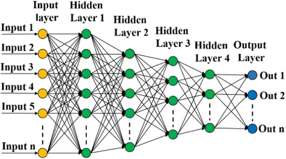
The DNN is used as a classifier. DNN is similar to Artificial neural configuration/network, consist of three layers: input, hidden, and output. Each layer is constructed by nodes, roughly modeled from nerve cell (neurons) in the brain. The different factors between neural networks and DNN are shown in the depth of the architectures (model). Typical DNN configuration is depicted in Figure 2.

Figure 2

General architecture of DNN.

As seen in Figure 2, the input layer is where the signal (sample) enters the DNN. The input layer has 256 elements, denoted as x = (Input 1, Input 2, … Input 256). Each node located in a hidden layer is linked with each input over the weights (shown as lines in Figure 2). In every node, in the hidden layer, the weight products are totaled and passed over a function as activation. The hidden layers are computed by h ^(t) (x). For the network with T hidden layers, the computation is as follows:

(2) f ( x ) = f [ a ( T + 1 ) ( h ( T ) ( a ( T ) ( ⋯ ( h ( 2 ) ( a ( 2 ) ( h ( 1 ) ( a ( 1 ) ( x ) ) ) ) ) ) ) ) ]

Every pre-activation function a ^(t)(x) is typically a linear operation with a matrix W ^(t) and bias b ^(t), which are capable of being combined into a parameter Φː

a ( t ) ( x ) = W ( t ) x + b ( t ) ,

a ( t ) ( x ˆ ) = F ( t ) x ˆ , t = 1 ,

a ( t ) ( h ˆ ( t − 1 ) ) = F ( t ) h ˆ ( t − 1 ) , t > 1 .

This “hat” denotes that the vector x has been appended with t. Hidden-layer activation functions h ^(t)(x) often have the same form at each level, but this is not a requirement.

In this study, supervised DNN will be utilized. The input for training is a time-based signal (sample), and the output is the type of broken bearing. The SoftMax layer is considered as output layer.

4 The proposed method

The proposed method (DTS–DNN) is anticipated in order to prevent pool operations in configuration of CNN for progressing the performance on diagnosing the broken bearing. DNN has a simpler arrangement, the configuration is set as 1D rather than 2D.

This complete work idea of this study is presented in Figure 3.

Figure 3

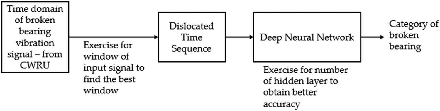
Whole idea of the work done in this study.

4.1 Architecture

The proposal for DTS–DNN configuration is portrayed in Figure 4. The DTS is already described in Section 3. DNN configuration contains four hidden layers that have nodes of are 256, 128, 64, and 32. This configuration is obtained based on trial and error. Initially, it is started by utilizing a neural network with one hidden layer configuration. The number 256 is obtained by seeing the signal form visually, where the number 256 already represents the shape of a one-wave signal. After observing its performance, and showing an accuracy that is still crisp, the hidden layers are added. The nodes number is half the nodes number in the previous hidden layer.

Figure 4

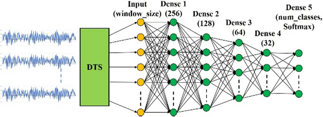
Proposed architecture of DTS–DNN.

The process of performance observation and addition of hidden layers continues until finally it matches the output layer of 16 nodes. The output layer denotes (presents) the broken bearing type.

For the proposed configuration, dislocated layer and DNN are utilized to extract the feature. SoftMax as a classifier is located in the last layer. The last output layer represents classification of broken bearing which is 16 categories. Adjustment of the weight (training) of both DNN and classifier (SoftMax) must be performed at the same time with the expectation to obtain minimum error between classifier and label in order to obtain higher accuracy. The DTS–DNN has more advantages to be applied for processing big data in industry because it is designed by using scheme of deep learning.

The deep learning mechanism is explained in Figure 5.

Figure 5

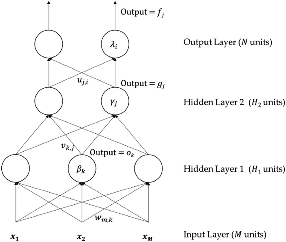
Typical configuration of DNN.

The final output is calculated as per equation (3) below, where β, γ, λ are bias, and σ is the activation function. The activation function is formulated in equation (5).

(3) f i = σ ∑ j = 1 H 2 u j , i σ ∑ k = 1 H 1 u k , j σ ∑ m = 1 M x m w m , k + β k + γ j + λ i .

Each class probability is provided by SoftMax function based on equation of activation function mentioned in equation (4).

(4) Soft Max ( Z i ) = exp ( Z i ) / ∑ j exp ( Z i ) ,

where Z represents the neuron values of the last output layer. These values are divided by the entirety of exponential values in arrange to normalize and after that change over them into probability.

4.2 Parameters optimization

In this proposal, activation function utilizes the rectified linear units (ReLU) function. Parameters are updated by utilizing Stochastic gradient descent algorithm (SGD) as an iterative method. SGD is one of the variations on the gradient descent method. Loss function utilizes categorical cross-entropy because there is only a category that is applied for each data point. The network is trained by utilizing back-propagation.

ReLUs are defined by mathematical equation (5).

(5) f ( x ) = 0 , x < 0 x , x ≥ 0 .

Categorical cross-entropy is a loss function that calculates the loss. With a number of datasets of n examples, the f _i(x) is a loss function with respect to the training example of index I, where x is the parameter vector. The objection function (lost function) is written in equation (6).

(6) f ( X ) = 1 n ∑ i = 1 n f i ( X )

The gradient of the objective function at x is calculated by using equation (7).

(7) ∇ f ( X ) = 1 n ∑ i = 1 n ∇ f i ( X ) .

If gradient descent is used, the computational cost for each independent variable iteration is б(n), which grows linearly with n. SGD reduces the computational cost at each iteration. At each iteration of SGD, an index i ∈ { 1 , … , n } is sampled uniformly for data examples at random, and the gradient ∇ f i ( x ) is computed to update x as per equation (8):

(8) X ← X − η ∇ f i ( X ) ,

where η is the learning rate. Computational cost for each iteration drops from б(n) of the gradient descent to the constant б(1). The stochastic gradient ∇ f i (x) is an unbiased estimate of the full gradient ∇f(x) because

(9) E i ∇ f i = 1 n ∑ i = 1 n ∇ f i ( X ) = ∇ f ( X ) .

Validation of the SGD is shown in Figure 6. In this case, the plot shows that the model seems to have converged. The line plots for cross-entropy show good convergence behavior, although somewhat bumpy. The model may be well configured giving no sign of over or under fitting.

Figure 6

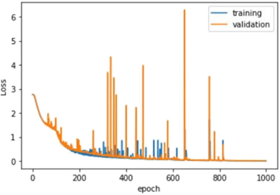
Plot for optimization performed by SGD.

5 Experimental design

Several simulations were performed by using data samples taken from CWRU that has Bearing Data Center [34]. Simulation was performed offline. These simulations utilized to verify the effectiveness of the DTS–DNN approach.

5.1 Proposed approach

The proposed method for this study is depicted in Figure 7.

Figure 7

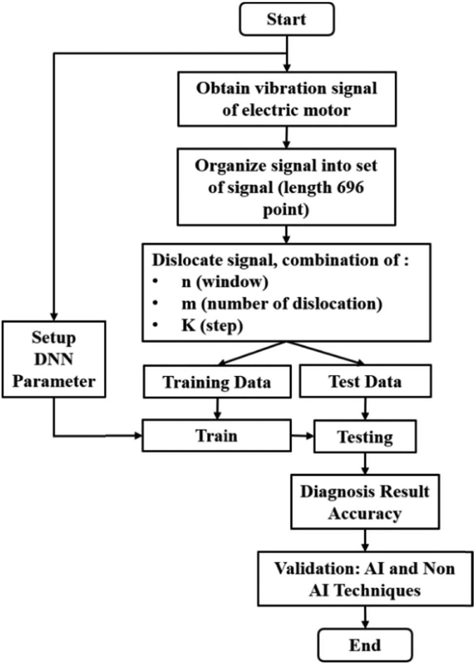
Flowchart of the proposed approach.

The steps are explained below:

Collect vibration signal from Bearing Data Center – CWRU. There are 16 signals representing 16 bearing conditions.
Organize signal. The length of each signal is 120,320 points or equivalents of 10.027 s. The signal is extracted to a sample with the length of each sample being 696 points (∼0.058 s).
Perform dislocations for variables n, m, and k.
Split data to two sets: data for training and data for testing. Proportion between training and testing shall be 80:20%.
Feed training data to DNN model for training.
Feed test data to trained DNN. The accuracy measured by confusion matrix.
Record the accuracy of the result.
Validate by benchmarking using both AI (Artificial Intelligence) and Non-AI techniques.

Note: training and testing were performed over and over to evaluate the impact of n, m, and k.

5.2 Vibration data description

The test bed configuration, components, and cross section are depicted in Figure 8. The configuration contains an electric induction motor that operates in three-phase electricity, turning around sensor, and a motor’s load. The ball bearing system has structure as shown on the right side. The ball bearing system has four main parts: external race, internal race, balls, and the cage encasing the balls for settling the balls.

Figure 8

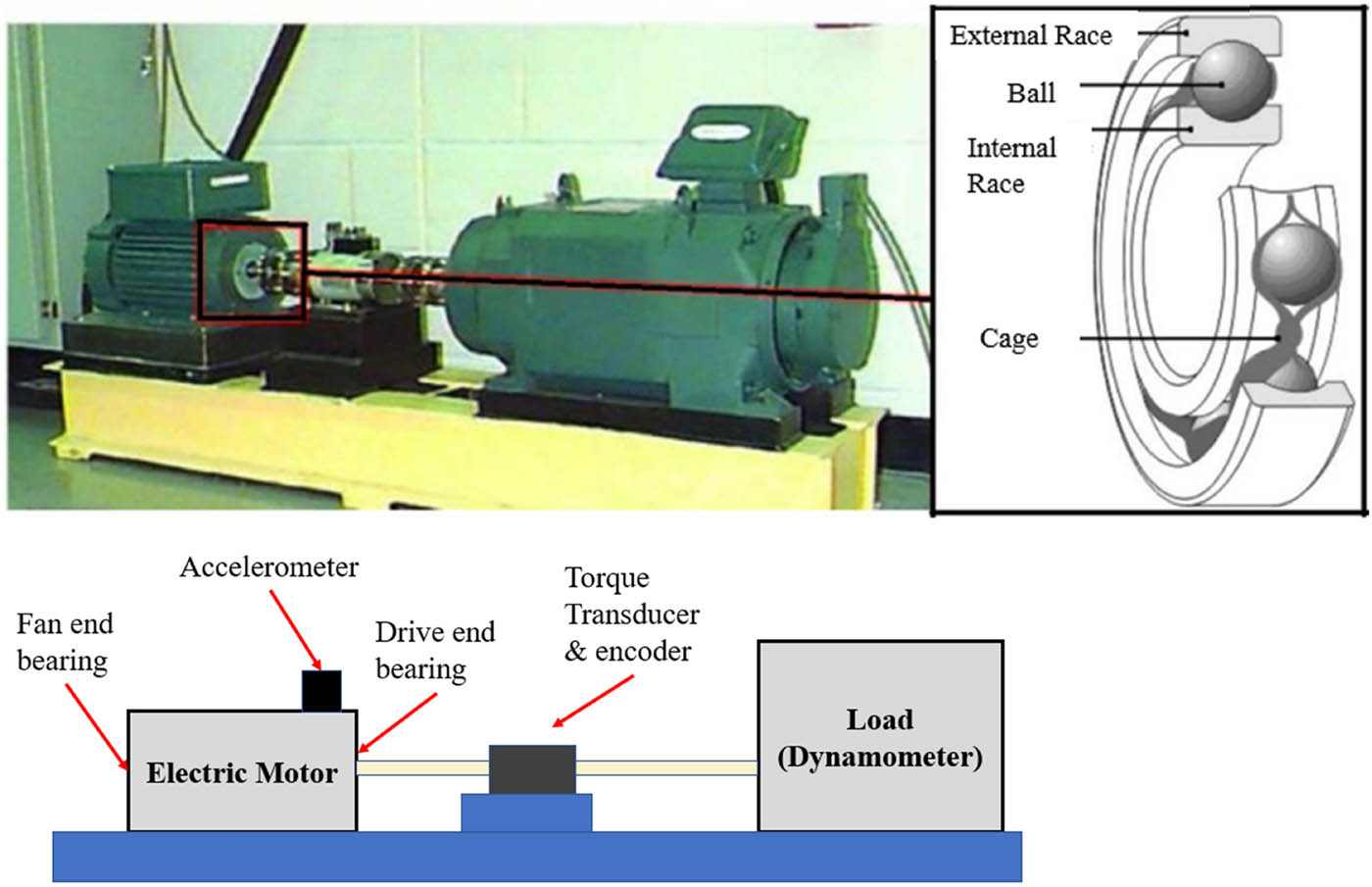
Test configuration.

Broken diameters consist of 0.007, 0.0014, 0.0021, and 0.0028 inches (1 inch = 25.4 mm). The sensor has a sampling rate of 12,000 Hz. The load taken is 0 hp. Single broken point is presented to the bearing utilizing electro-discharge machining.

Table 2 presents 16 condition for rolling bearing operation. The condition includes datasets for normal bearing, ball or rolling broken element, broken internal race, and broken external race. The broken external race is divided into three categories according to the broken position relative to the stack zone: “center” (broken position in the 6.00 o’clock), “orthogonal” (broken position in the 3.00 o’clock), and “opposite” (broken position in the 12.00 o’clock). The datasets are categorized by broken size (0.007–0.0028 inches).

Table 2

Operation conditions of bearing

No.	Operation condition	Broken diameter (inch)	External race broken orientation	Label of condition
1	Not broken	0.000″	—	0
2	Ball bearing	0.007″	—	1
3	Ball bearing	0.01″	—	2
4	Ball bearing	0.021″	—	3
5	Ball bearing	0.028″	—	4
6	Internal	0.007″	—	5
7	Internal	0.014″	—	6
8	Internal	0.021″	—	7
9	Internal	0.028″	—	8
10	External	0.007″	Vertical@3:00	9
11	External	0.007″	Center@6:00	10
12	External	0.007″	Opposite@12:00	11
13	External	0.014″	Center@3:00	12
14	External	0.021″	Vertical@3:00	13
15	External	0.021″	Center@6:00	14
16	External	0.021″	Opposite@12:00	15

The dataset used is secondary data downloaded from Bearing Data Center which is widely used for benchmarking diagnostic performance of bearing faults diagnosis. There is no missing value in the data.

The data are labeled. Refer to data record, the range of diagnosable is very broad from very easily diagnosable to not diagnosable. Datasets are exhibited from stationary to very non-stationary characteristics [35].

5.3 Variation in “s,” “m,” and window

The variations in “s,” “m,” and window (data point) are depicted in Table 3. There are 24 exercises for variation in “s,” “m,” and window.

Table 3

Variations in “s,” “m,” and window

s	m	Window (data point)
16	8	64	128	224	248	256	320
16	4	64	128	224	248	256	320
8	8	64	128	224	248	256	320
8	4	64	128	224	248	256	320

The value of m is determined based on the criteria that m × s is less or multiple periods of signal. For this research, m values are 4 and 8.

The window (w) is selected based on visual predictions of cyclical period of signal. Initial value of w is 256 based on visual observation. Visually, the cyclical period of the signal is 256. Value 248 used as a variation in 256 to anticipate actual cyclical period is little bit less than 256. Henceforth, the window value is the addition and subtraction for multiples of 64.

The initial s value is 8 based on DTS–CNN, where s = 8 produces the worst accuracy due to too much overlap [28]. The second value of s is 16 with the expectation to reduce the overlap.

5.4 Validation and benchmarking

The performance of DTS–DNN is validated using randomly repeated cross training-testing validation method with accuracy metric and benchmarked using other AI techniques and non-AI techniques. There are several AI techniques used to perform this benchmarking comparison, ranging from shallow and deep architectural techniques: support vector classifier (SVC), decision trees classifier, random forest classifier, naïve Bayes classifier, K-nearest neighbors (KNN), and DBN.

In shallow architecture, the raw signal will be transformed first into a frequency domain signal by utilizing the algorithm of Fast Fourier Transformation (FFT) before being fed to AI. These frequency domain signals are used to classify manually using non-AI techniques that were per-formed by using the mean of the selected frequency signal.

6 Results and discussion

This case study focuses on DTS–DNN for broken bearing diagnosis without manual feature selection.

6.1 Dislocated operation

The data used are secondary data taken from CWRU. There are 16 signals representing 16 bearing conditions. The signal length is 120,320 points, which is equal to signal length of 10.027 s. Each signal is divided into samples with a length of 696 points. This division is shown in Figure 9.

Figure 9

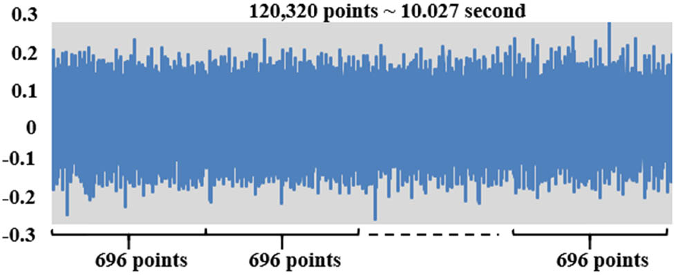
Signal Division.

The dislocated operation or working procedure is shown in Figure 10. From Figure 10, it can be seen that the extracted signal is performed each time. Signal has a length of w or n. The first extracted sample is started at point 0 (0 × s or k).

Figure 10

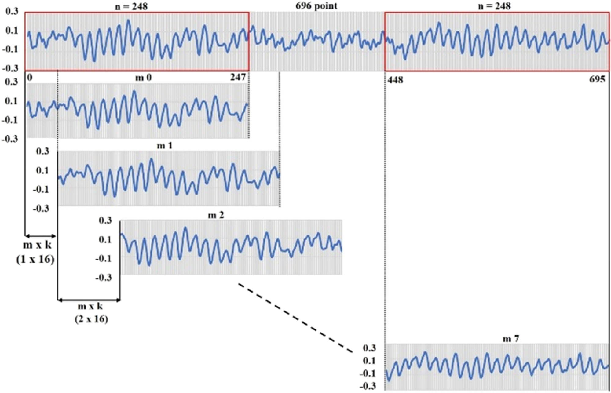
Dislocated operation.

The next sample is extracted starting at point s (1 × s). Then, translate 2 × s distance and excerpt other signals with the same length. Next translating 3 × s distance, next 4 × s distance, and so on. The number of translation is m × s distance and excerpts other signals. The extracted sample is then fed to DNN for classification process.

6.2 Training and testing

The network was trained by using 17,536 training data and tested by using 4,480 testing data (20%). For the best candidate, it was randomly repeated 15 times. Sixteen class classification problems are solved without overfitting phenomena. The obtained accuracy result is depicted in Figure 11. The model accuracy is depicted in Figure 12.

Figure 11

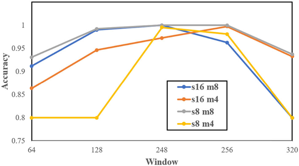
Comparison among “s,” “m,” and window.

Figure 12

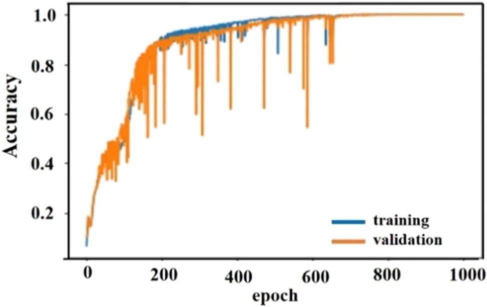
Model accuracy.

From Figure 11, it appears that windows 248 and 256 can produce an accuracy of 100%, namely, at s = 16 m = 8 (window 248) and s = 8 m = 8 (window 256). Narrowing (128, 64) and widening (320) of the window does not improve accuracy. It means that cyclical period of vibration signal is close or near to 248 and 256. It took approximately 0.02 s. A shortening or narrowing window will not capture all information in a cyclical period, while widening the window will mix information among cyclical periods.

The best combination is window 248, with s = 16 and m = 8. The performance test is carried out by using 15 random splits of training and test data, by using the same parameter window, w = 248, with s = 16 and m = 8. On average, the accuracy is 0.9942 with a standard deviation of 0.0149.

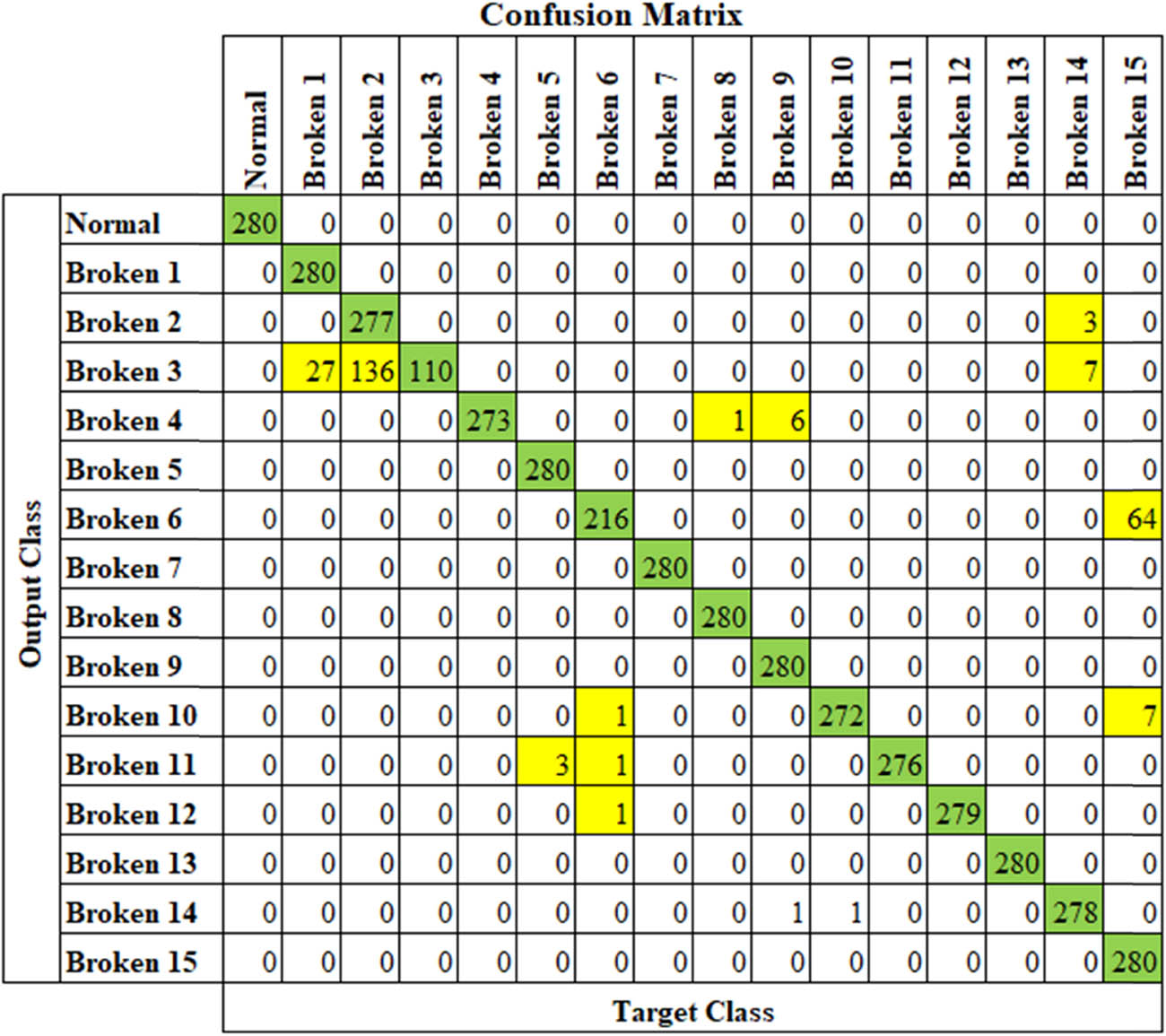
The performance of DTS–DNN is measured by using a confusion matrix. Confusion matrix for the good and worst performance is shown in Figures 13 and 14, respectively.

Figure 13

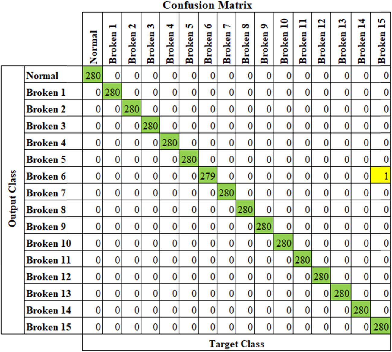
Confusion matrix for good performance model.

Figure 14

Confusion Matrix for worst performance model.

DTS–DNN performs well (99.4% average accuracy). DTS–DNN performs as a classifier at raw signal level that utilizes raw signals as the feed/input directly. Additional process for extracting features as the feeding to classifier is not required. The whole data of the signal was kept. The features could be learned automatically and directly by the model, without any human intervention.

6.3 Comparison with other AI techniques

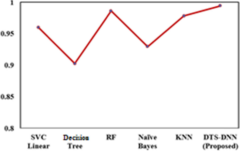
Comparisons were performed by using shallow AI /ML technique based on frequency domain that produced better accuracy than time domain. The dislocated samples are transformed to frequency domain, and then fed to shallow AI which are SVC linear, decision tree, RF, naïve Bayes, and KNN. The comparison is presented in Figure 15. The DTS–DNN is still competitive comparing to shallow AI/ML.

Figure 15

Comparison with shallow AI.

The proposed method is also compared by using the same experimental database on deep learning methods. This experiment utilized the same database used by Shao et al. [31] that came from CWRU’s Bearing Data Center. Both these experiments and Shao used the same number of bearing fault classes (16 classes).

Compared to shallow AI architecture and DBN as deep learning, the benefit of DTS–DNN is the capability to utilize time domain raw signal without any conversion or transformation to other signals such as frequency domain or wavelet-based. This DTS–DNN can overcome CNN’s weakness, which is the pool operation which can eliminate information. While in DNN, every node is configured to be connected, and all information are still available (no information is lost).

The comparison to DBN with DTCWPT is depicted in Table 4 [31].

Table 4

Bearing operation conditions

Items	Shao (DBN)	Proposed (DTS–DNN)
Dataset	CWRU	CWRU
Raw data	Vibration	Vibration
Input	Time–frequency	Time based
Deep learning	DBN	DNN
Classes	16	16
Accuracy	95.22%	99.42%

6.4 Comparison with non-AI techniques

Validation is done by using the frequency domain signal. Time-based signal is first transformed into a frequency-based signal by using FFT. Figure 16 depicts an example of the original time domain signal that is similar to the signal used by DTS–DNN. The transformed result is shown in Figure 17.

Figure 16

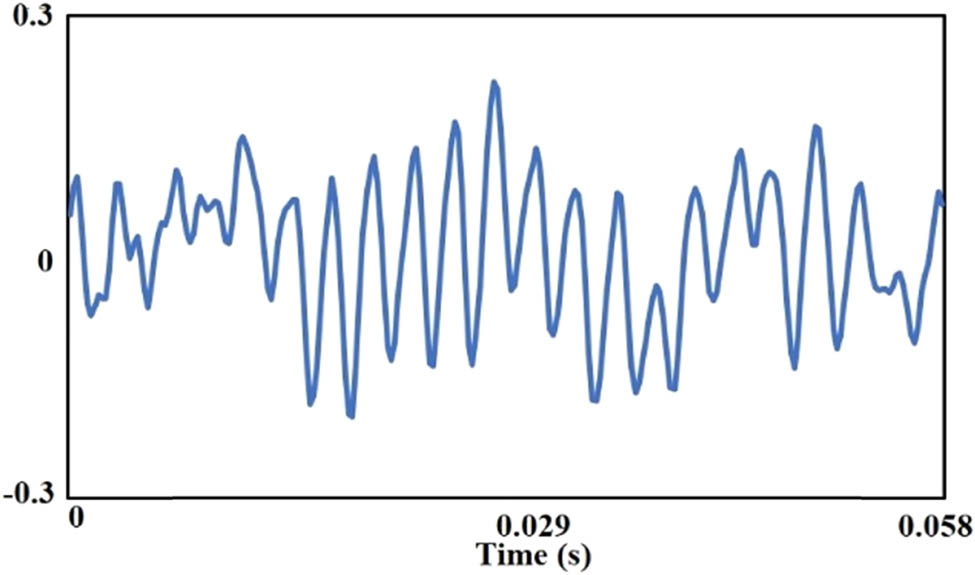
Time domain signal (normal bearing).

Figure 17

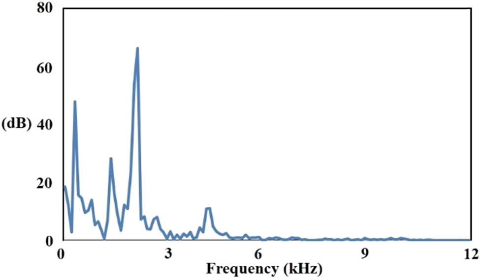
Frequency domain signal (normal bearing).

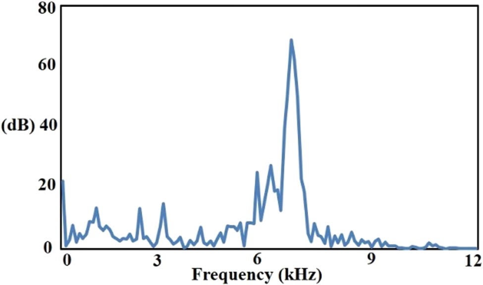
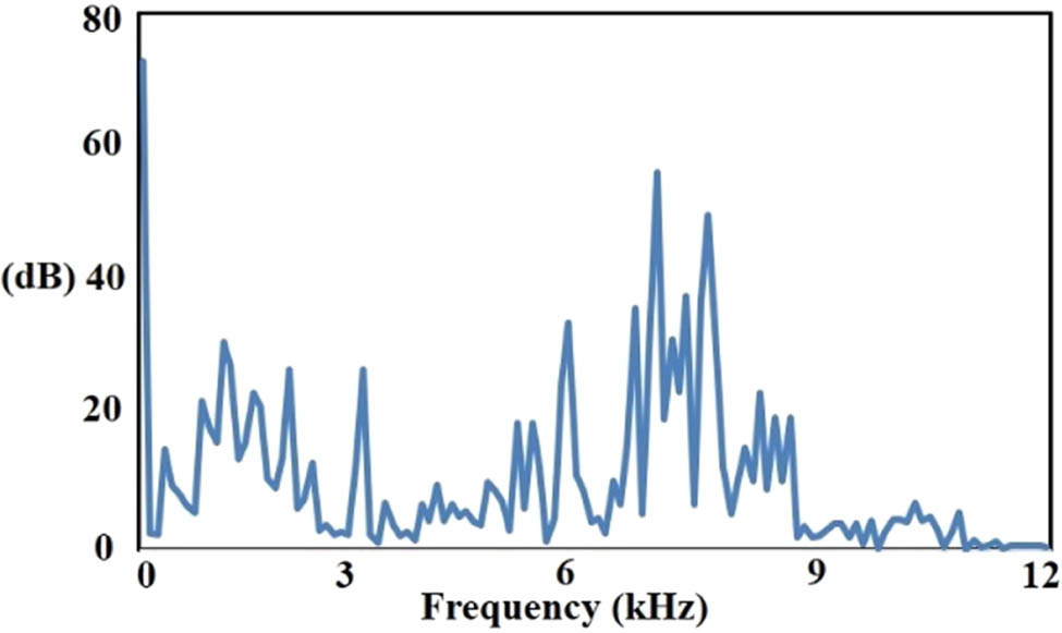
The example of frequency domain signal for broken ball component, broken internal race, and broken external race are depicted in Figures 18–20.

Figure 18

Frequency domain signal (broken ball).

Figure 19

Frequency domain signal (broken internal race).

Figure 20

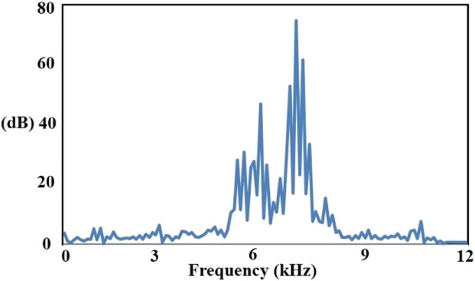
Frequency domain signal (broken external race).

Classification for non-AI was performed manually by using the mean of selected frequency. The result is shown in Table 5, and it is not competitive with AI techniques. The non-AI shall involve proper domain or subject matter expert for better result.

Table 5

Comparison of accuracy with non-AI technique

Items	Non-AI	Proposed (DTS–DNN)
Dataset	CWRU	CWRU
Raw data	Vibration	Vibration
Input	Frequency	Time based
Classes	16	16
Accuracy	25.3%	99.42%

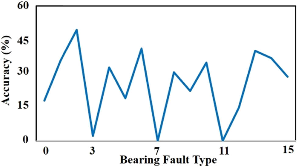
The accuracy for each broken bearing type is shown in Figure 21. This result is aligned with study results performed by Smith that the data for broken bearing extended from exceptionally simple diagnosable to not diagnosable. This result supports the need for developing better methods such as DTS–DNN.

Figure 21

Accuracy for each broken bearing (bearing fault) type.

7 Conclusion

Proposed method (DTS–DNN) has been offered to diagnose broken bearing of electric induction motor and produce higher accuracy (99.4% average accuracy). DTS–DNN becomes a promising alternative for broken bearing diagnosis by using raw signals directly without any human-crafted features. The overfitting could be mitigated because every node in the hidden layer is connected to each input through the weights. The cyclical period of the signal used in this research is approximately 0.02 s. Window sampling (k) should be chosen appropriately, and close to a cyclical period of signal to have a better result.

8 Recommendation

DTS–DNN is a potential method that could be utilized in other applications, not only for processing vibration signals. For future work, authors recommend to assess the possibility of implementation of DTS-DNN in other types of electrical motor and other rotating /moving machine, and also, to assess the possibility to utilize DTS–DNN in other similar signals such as electrocardiogram.

Acknowledgments

The authors extend their sincere appreciation and thanks to the Case Western Reserve University) for providing the experimental data of bearing vibration as free access.

Funding information: This research received no external funding.
Author contributions: Conceptualization, Noor Akhmad Setiawan and Pramudyana Agus Harlianto; methodology, Noor Akhmad Setiawan and Pramudyana Agus Harlianto; software, Pramudyana Agus Harlianto; validation, Noor Akhmad Setiawan, Pramudyana Agus Harlianto, and Teguh Bharat Adji; investigation, Pramudyana Agus Harlianto; resources, Pramudyana Agus Harlianto; writing – prepare original draft, Pramudyana Agus Harlianto; writing – review and editing, Noor Akhmad Setiawan and Teguh Bharata Adji; visualization, Pramudyana Agus Harlianto; supervision, Noor Akhmad Setiawan and Teguh Bharata Adji. All authors have read and agreed to the published version of the manuscript.
Conflict of interest: The authors declare no conflict of interest.

References

[1] Marcelo C, Terra I. Fault diagnosis of induction motors based on FFT. Fourier Transform - Signal Processing; 2012. 10.5772/37419.Suche in Google Scholar

[2] Daviu JA, Aviyente S, Strangas EG, Riera Guasp M. Scale invariant feature extraction algorithm for the automatic diagnosis of rotor asymmetries in induction motors. IEEE Trans Ind Inform. 2013;9(1):100–8. 10.1109/TII.2012.2198659.Suche in Google Scholar

[3] Gao Z, Cecati C, Ding SX. A survey of fault diagnosis and fault-tolerant techniques Part I: Fault diagnosis. IEEE Trans Ind Electron. 2015;62(6):3768–74. 10.1109/TIE.2015.2417501.Suche in Google Scholar

[4] Patel RK, Giri VK. Feature selection and classification of mechanical fault of an induction motor using random forest classifier. Perspect Sci. 2016;100(8):334–7. 10.1016/j.pisc.2016.04.068.Suche in Google Scholar

[5] Konar P, Chattopadhyay P. Bearing fault detection of induction motor using wavelet and support vector machines (SVMs). Appl Soft Comput. 2011;11(6):4203–11. 10.1016/j.asoc.2011.03.014.Suche in Google Scholar

[6] Vakharia V, Gupta VK, Kankar PK. Ball bearing fault diagnosis using supervised and unsupervised machine learning methods. Int J Acoust Vib. 2015;20(4):244–50. 10.20855/ijav.2015.20.4387.Suche in Google Scholar

[7] Kankar PK, Sharma SC, Harsha SP. Fault diagnosis of ball bearings using machine learning methods. Expert Syst Appl. 2011;38(3):1876–86. 10.1016/j.eswa.2010.07.119.Suche in Google Scholar

[8] Aggarwal A, Malik H, Sharma R, Feature Extraction using EMD and Classification through Probabilistic Neural Network for Fault Diagnosis f Transmission Line, 2016 IEEE 1st International Conference on Power Electronics, Intelligent Control and Energy Systems (ICPEICES), 2016, p. 1–6, doi: 10.1109/ICPEICES.2016.7853709.10.1109/ICPEICES.2016.7853709Suche in Google Scholar

[9] Malik H, Mishra S, Extreme learning machine-based fault diagnosis of power transformer using IEC TC10 and its related data, 2015 Annual IEEE India Conference (INDICON), 2015, pp. 1–5, doi:10.1109/INDICON.2015.7443245.10.1109/INDICON.2015.7443245Suche in Google Scholar

[10] Heda Z. Fault diagnosis and life prediction of mechanical equipment based on artificial intelligence. J Intell Fuzzy Syst. 2019;37(3):3535–44. 10.3233/JIFS-179157.Suche in Google Scholar

[11] Prieto MD, Cirrincione G, Espinosa AG, Ortega JA, Henao H. Bearing fault detection by a novel condition monitoring scheme based on statistical time features and neural networks. IEEE Trans Ind Electron. 2013;60(8):3398–407. 10.1109/TIE.2012.2219838.Suche in Google Scholar

[12] Huang NE, Shen Z, Long SR, Wu ML, et al. The empirical mode decomposition and the Hilbert spectrum for nonlinear and non-stationary time series analysis. R Soc Publ. 1998;454(1971):903–95. 10.1098/rspa.1998.0193.Suche in Google Scholar

[13] Yan R, Gao RX, Chen X. Wavelets for fault diagnosis of rotary machines: A review with applications. Signal Process. 2014;96:1–15. 10.1016/j.sigpro.2013.04.015.Suche in Google Scholar

[14] Ning J, Yao C, Yunyang L, Youyuan T, Intelligent fault diagnosis of rotating machines based on wavelet time-frequency diagram and optimized stacked denoising auto-encoder. IEEE Sens J. 2022;22(17):17139–50.10.1109/JSEN.2022.3193943Suche in Google Scholar

[15] Lei Y, Lin J, He Z, Zuo MJ. A review on empirical mode decomposition in fault diagnosis of rotating machinery. Mech Syst Signal Process. 2013;35(1–2):108–26. 10.1016/j.ymssp.2012.09.015.Suche in Google Scholar

[16] Cui H, Guan Y, Chen H. Rolling element fault diagnosis based on VMD and sensitivity MCKD. IEEE Access. 2021;9:120297–308. 10.1109/ACCESS.2021.3108972.Suche in Google Scholar

[17] Chen SS, Donoho DL, Saunders MA. Atomic decomposition by basis pursuit. Soc Ind Appl Mathematics. 2001;43(1):129–59, https://web.stanford.edu/group/SOL/papers/BasisPursuit-SIGEST.pdf.10.1137/S003614450037906XSuche in Google Scholar

[18] Van M, Jun KHee. Bearing defect classification based on individual wavelet local fisher discriminant analysis with particle swarm optimization. IEEE Trans Ind Inform. 2015;64(12):124–35. 10.1109/TII.2015.2500098.Suche in Google Scholar

[19] Liu R, Yang B, Zhang X, Wang S, Chen X. Time-frequency atoms-driven support vector machine method for bearings incipient fault diagnosis. Mech Syst Signal Process. 2016;75:345–70. 10.1016/j.ymssp.2015.12.020.Suche in Google Scholar

[20] Agrawal S, Giri VK, Giwari AN. Induction motor bearing fault classification using WPT, PCA and DSVM. J Intell Fuzzy Syst. 2018;35(5):5147–58. 10.3233/JIFS-169798.Suche in Google Scholar

[21] Gunerkar RS, Jalan AK, Belgamwar SU. Fault diagnosis of rolling element bearing based on artificial neural network. J Mech Sci Technol. 2019;33:505–11. 10.1007/s12206-019-0103-x.Suche in Google Scholar

[22] Tobon Mejia DA, Medjaher K, Zerhouni N, Tripot G. A data-driven failure prognostics method based on mixture of Gaussian hidden Markov models. IEEE Trans Reliab. 2012;61(2):491–503. 10.1109/TR.2012.2194177.Suche in Google Scholar

[23] Yu J. Local and nonlocal preserving projection for bearing defect classification and performance assessment. IEEE Trans Ind Electron. 2012;59(5):2363–76. 10.1109/TIE.2011.2167893.Suche in Google Scholar

[24] Duan L, Xie M, Wang J, Bai T. Deep learning enabled intelligent fault diagnosis: Overview and applications. J Intell Fuzzy Syst. 2018;35(5):5771–84. 10.3233/JIFS-17938.Suche in Google Scholar

[25] Jia F, Lei Y, Lin J, Zhou X, Lu N. Deep neural networks: A promising tool for fault characteristic mining and intelligent diagnosis of rotating machinery with massive data. Mech Syst Signal Process. 2016;72:303–15. 10.1016/j.ymssp.2015.10.025.Suche in Google Scholar

[26] Janssens O, Slavkovikj V, Vervisch B, Stockman K, Loccufier M, Verstockt S, et al. Convolutional neural network-based fault detection for rotating machinery. J Sound Vib. 2016;377:331–45. 10.1016/j.jsv.2016.05.027.Suche in Google Scholar

[27] Zhu D, Zhang Y, Zhao L. Fault diagnosis method for rolling element bearing with variable rotating speed using envelope order spectrum and convolutional neural network. J Intell Fuzzy Syst. 2019;37(2):3027–40. 10.3233/JIFS-190101.Suche in Google Scholar

[28] Liu R, Meng G, Yang B, Sun C, Chen X. Dislocated time series convolutional neural architecture: An intelligent fault diagnosis approach for electric machine. IEEE Trans Ind Inform. 2016;13(3):1310–20. 10.1109/TII.2016.2645238.Suche in Google Scholar

[29] Li C, Sánchez RV, Zurita G, Cerrada M, Cabrera D. Fault diagnosis for rotating machinery using vibration measurement deep statistical feature learning. Sensors Switz. 2016;16(6):895. 10.3390/s16060895.Suche in Google Scholar PubMed PubMed Central

[30] Shao H, Jiang H, Zhao H, Wang F. A novel deep autoencoder feature learning method for rotating machinery fault diagnosis. Mech Syst Signal Process. 2017;95:187–204. 10.1016/j.ymssp.2017.03.034.Suche in Google Scholar

[31] Shao H, Jiang H, Wang F, Wang Y. Rolling bearing fault diagnosis using adaptive deep belief network with dual-tree complex wavelet packet. ISA Trans. 2017;69:187–201. 10.1016/j.isatra.2017.03.017.Suche in Google Scholar PubMed

[32] Hearty J. Advanced Machine Learning with Python. PACKT Publishing Ltd; I. Birmingham - Mumbai. 2016. https://www.amazon.com/Advanced-Machine-Learning-Python-Hearty/dp/1784398632.Suche in Google Scholar

[33] Levine S, Finn C, Darrell T, Abbeel P. End-to-end learning of deep visuomotor policies. J Mach Learn Res. 2016;17:1–40, https://arxiv.org/abs/1504.00702.Suche in Google Scholar

[34] Case Western Reserve University Bearing Data Center. [Online]. Available: http://csegroups.case.edu/bearingdatacenter/home. [Accessed: 22-Oct-2017].Suche in Google Scholar

[35] Smith WA, Randall RB. Rolling element bearing diagnostics using the Case Western Reserve University data: A benchmark study. Mech Syst Signal Process. 2015;64–5:100–31. 10.1016/j.ymssp.2015.04.021.Suche in Google Scholar

Received: 2022-10-11

Revised: 2022-12-10

Accepted: 2023-01-04

Published Online: 2023-03-31

This work is licensed under the Creative Commons Attribution 4.0 International License.

Artikel in diesem Heft

https://doi.org/10.1515/eng-2022-0402

Schlagwörter für diesen Artikel

dislocated time sequences; deep neural network; broken bearing diagnosis; accuracy; multi-class

Creative Commons

BY 4.0

s	m	Window (data point)
16	8	64	128	224	248	256	320
16	4	64	128	224	248	256	320
8	8	64	128	224	248	256	320
8	4	64	128	224	248	256	320

s	m	Window (data point)
16	8	64	128	224	248	256	320
16	4	64	128	224	248	256	320
8	8	64	128	224	248	256	320
8	4	64	128	224	248	256	320

s	m	Window (data point)
16	8	64	128	224	248	256	320
16	4	64	128	224	248	256	320
8	8	64	128	224	248	256	320
8	4	64	128	224	248	256	320