1D-CNN: Classification of normal delivery and cesarean section types using cardiotocography time-series signals
-
Vidya Sujit Kurtadikar
 und
Himangi Milind Pande
und
Himangi Milind Pande

Abstract
Cardiotocography (CTG) is considered the gold standard for monitoring fetal heart rate (FHR) during pregnancy and labor to estimate the danger of oxygen deprivation. Visual interpretation of CTG traces is complex and frequently results in high rates of false positives and false negatives, leading to unfavorable and unwanted outcomes such as fetal mortality or needless cesarean surgery. If the data are well-balanced, which is uncommon in medical datasets, machine learning techniques can be helpful in interpretation. This study is designed to determine classification performance under various data balance approaches. We propose a robust methodology for the automated extraction of features that use a deep learning model based on the one-dimensional convolutional neural network (1D-CNN). We used a public database containing 552 intrapartum CTG recordings. Due to the imbalance in the dataset, the experiments were conducted under a variety of conditions such as (i) an unbalanced dataset, (ii) undersampling, (iii) a weighted binary cross-entropy approach, and (iv) oversampling utilizing the synthetic minority oversampling technique (SMOTE). We found an excellent sensitivity (99.80% for the unbalanced dataset, 96.25% for the weighted binary cross-entropy approach, and 99.81% with SMOTE) except for the under sampling situation, in which the sensitivity was 85.71%. Moreover, the 1D-CNN model incorporating SMOTE yielded promising results in 88% specificity, 93.72% quality index (QI), and 95.10% area under the curve. The model exhibited excellent performance in terms of sensitivity in every scenario except for undersampling. The oversampling of training data with SMOTE yielded a decent level of specificity, demonstrating the model’s strong predictive capacity. In addition, the SMOTE scenario resulted in fewer training epochs, which is another accomplishment.
1 Introduction
According to the World Health Organization’s statistical data, 2.4 million infant deaths occurred in the first month of life in 2020. Preterm delivery, issues during childbirth (birth asphyxia or lack of breathing), infections, and congenital disabilities accounted for most neonatal deaths in 2019 [1]. Fetal health is assessed during antepartum and intrapartum to diagnose hypoxia, the early stage of asphyxia. Experts and gynecologists use the Cardiotocography (CTG), which employs Doppler ultrasound and pressure sensors to monitor fetal heart rate (FHR) and uterine contraction (UC) noninvasively to evaluate fetal well-being. Although various standards for CTG interpretations exist, [2–4], the structure of the guidelines varies. These changes significantly impact observer agreement and dependability [5]. In addition, the intricate structure of CTG traces makes visual interpretation difficult, increasing the false-positive rate and resulting in unnecessary surgical births and cesarean sections [6,7]. Computer scientists have researched many semi-automatic and automatic algorithms to address these limitations. These algorithms extract trustworthy and vital information by leveraging all the untapped latent in the FHR and UC signals to enhance diagnostic efficacy [8–12]. Modern CTG interpretation studies emphasize objective approaches leveraging machine and deep learning. The present study utilized a deep learning method based on the one-dimensional convolutional neural network (1D-CNN) technique, which is well known for automatic feature extraction [13]. In addition, the imbalance in the dataset is addressed using various approaches. Therefore, the contributions of this work are multifold, as given below:
The current study is likely the first to experiment with and evaluate alternative scenarios based on the imbalance of the dataset.
Feature extraction is performed automatically using the 1D-CNN deep learning model.
The total training time is minimized in the SMOTE situation because very few epochs are required.
2 Literature review
The notable research based on machine and deep learning methods for analyzing CTG signals is mentioned here. Using the least-squares support vector machine (LS-SVM)-based model and particle swarm optimization [14] classified CTG traces into normal, suspect, and pathological classes with 91.62% accuracy. However, additional helpful evaluation criteria, such as sensitivity and a specificity, must be added. The categorization of FHR signals utilizing generative models (GMs) and Bayesian theory on private datasets yielded a sensitivity of 81.7% and a specificity of 60.0% [15]. The sparse SVM model led to classification results of 73% sensitivity and 75% specificity [16]. An ensemble classifier consisting of SVM, random forest (RF), and Fisher’s linear discriminant analysis (FLDA) classifiers resulted in a sensitivity of 87%, a specificity of 90%, area under the curve (AUC) of 96%, and a mean squared error of 9% [17]. Artificial neural networks performed admirably, with a sensitivity of 99.73% and a specificity of 97.94% as compared to other machine learning techniques [18]. The convolutional neural network (CNN) model with an AUC of 82% surpassed long short-term memory in [19]. For a private dataset, the CNN classifier achieved an accuracy of 93.24% [20]. The features were created using multivariate intrinsic mode functions to extract nonlinear and nonstationary relationships from FHR-UC signals [21]. The AdaBoost classifier achieved a sensitivity of 91.8%, a specificity of 95.5%, and, an AUC of 98% using those features. A sensitivity of 77.40% and a specificity of 93.86% were obtained using 12 pertinent features and the SVM model after testing with various feature selection methods and machine learning models [22].
Using the multimodal convolutional neural network (MCNN) model and the stacked MCNN model to classify an extensive private database, Petrozziello et al. [23] found that the MCNN model performed better. The recurrence plot transformed an FHR signal from one dimension to two dimensions. The classes were balanced by choosing a small number of matching records from each class, and the image dataset was enriched by modifying several recurrence plot parameters. CNN classifier attained 98.69% accuracy, 99.29% sensitivity, 98.10% specificity, and 98.70% AUC [24]. Several machine learning models used a mixture of traditional and common spatial pattern features as input, and the SVM classifier produced the best results with 74.29% sensitivity, 99.55% specificity, and 94.75% accuracy [25]. The bagging ensemble achieved 99.02% classification accuracy, a 99% F1-Score, and a 99.99% AUC [26]. The segmentation approach was employed for class balance, and CNN classification yielded an 80% sensitivity, 79% specificity, and 86% AUC [27]. The generative adversarial network (GAN) is used to augment FHR signals to handle the data imbalance problem, yielding 71.08% accuracy, 67.64% sensitivity, and 71.97% specificity [28]. The machine learning model has associated shortcomings in selecting optimal features, which is often complex, time-consuming, and requires skill. Recently, deep learning techniques have proven effective in a variety of real-world applications [29–31] for acquiring relevant and essential information without bias. Based on a 1D-CNN, we suggest a deep learning model, considering the significant benefits of autonomous feature learning and cutting-edge performance for one-dimensional data [13]. The experiment utilized an open-access dataset collected by the Czech Technical University (CTU) in Prague and the University Hospital in Brno (UHB) [32,33]. The dataset is unbalanced regarding cases and controls, including 46 cesarean section births (cases) and 506 vaginal births (controls). We conducted experiments to address this imbalance, considering various scenarios, including:
Considering the dataset without any balancing method (unbalanced dataset).
Undersampling the records from the control group to match the case group.
Using the weighted binary cross-entropy method, which assigns weights to classes such that one misclassification from the case category contributes to as many as 11 misclassifications in the control category (considering 46 cases vs 506 controls in the dataset).
Oversampling the minority class using the SMOTE [34], which is based on a combination of oversampling the minority group records and undersampling the majority group records. The oversampling uses k-nearest neighbors to generate synthetic examples in the feature space.
3 Materials and methods
This section explains the dataset used for various testing settings, the input normalization method used to normalize the FHR signal, and the network architecture employed in this study.
3.1 Dataset
The current study utilized the CTU-UHB intrapartum CTG dataset, freely available at Physionet [32,33]. The dataset comprised 552 intrapartum CTG samples carefully obtained from singleton pregnancies without known congenital disabilities or intrauterine growth restrictions. The significant attributes of the sample and attribute distributions are depicted in Table 1. The dataset consists of 506 recordings delivered vaginally, considered normal delivery cases (control group) in the current study, whereas 46 recordings were delivered by cesarean section (case group). Each record also contains FHR in bpm and UC in mmHg time-series data with a 4 Hz sampling frequency. The recordings are 90 min at maximum and are started at most 90 min prior to delivery. The second phase of labor took up to 30 min. The FHR signal served as the input layer for the 1D-CNN model in the current work under all data balance conditions discussed in Section 5. The present study aims to classify FHR signals in normal delivery and cesarean section records. Each record’s delivery-type parameter is considered the gold standard for the classification. The FHR pre-processing used in the current study is explained in Section 3.2.
The patient’s major parameters and statistics available in the CTU-UHB Database [32]
| Parameter name | Mean (Median) | Min | Max |
|---|---|---|---|
| Mother’s age (years) | 29.8 | 18 | 46 |
| Parity | 0.43 (0) | 0 | 7 |
| Gravidity | 1.43 (1) | 1 | 11 |
| Gestational age (weeks) | 40 | 37 | 43 |
| pH | 7.23 | 6.85 | 7.47 |
| Base excess |
|
|
|
| Base deficit in extracellular fluid (BDecf, mmol/l) | 4.60 |
|
|
| Apgar score (1 min) | 8.26 (8) | 1 | 10 |
| Apgar score (5 min) | 9.06 (10) | 4 | 10 |
| Infant weight (kg) | 3.408 | 1.970 | 4.750 |
| Infant sex (Female/Male): 259 / 293 | |||
| Type of delivery: Normal (vaginal) = 506, Cesarean section = 46 |
3.2 Dataset pre-processing
The movement of pregnant women and fetus, as well as incorrect sensor placement, can introduce noise in the FHR signal. The classification efficiency is highly influenced by input quality; therefore, the pre-processing phase is of utmost importance. The pre-processing used in this article is based on [24], where missing values were linearly interpolated, and missing values that lasted longer than 15 s were removed directly. If the absolute difference of two adjacent values was greater than 25 bpm, then interpolation was carried out between the initial sampling point and the first point of the next stable part. In addition, FHR values larger than 200 bpm or less than 50 bpm were considered extreme points and eliminated. The linear interpolation was used to fill up the corresponding segment.
3.3 Input normalization
The normalization method changes the features to a similar scale, which is essential to improve the classification model’s performance and training stability. This work employed the
In equation (1),
3.4 1D-CNN
Due to the unique property of combining feature mining and labeling procedures within one learning frame, 1D-CNNs have recently gained popularity in a variety of signal-processing applications. Compared to traditional multilayer perceptron (MLP) networks, it can process inputs with high efficacy. CNN has high fault tolerance and robustness and is simple to train and optimize [13].
The core CNN design contains an input layer, a convolution layer, a pooling layer, a fully linked layer, and an output layer. Figure 1 depicts the model employed in this research. A pair of convolution and max pooling layers were employed, succeeded by a layer that flattened the 1D-CNN to facilitate the creation of the fully connected MLP. The MLP comprised two dense layers consisting of 10 neurons and one neuron each, which were fully connected. Concerning binary classification, sigmoid activation was utilized in the output layer to classify the FHR signal input into normal and abnormal classes. At the convolution layer, rectified linear unit (ReLU) activation was applied. The parameter tuning was carried out for the convolution layer’s two essential parameters: the number of filters (denoted by variable n_filters) and the kernel size (denoted by variable kernel_s). The values of those parameters were determined empirically, as discussed in Section 5. The He initialization method was employed to initialize the kernel weights. The batch normalization enhanced the efficiency of the deep neural network concerning the training period and overall stability. The layer-wise parameter settings for the proposed 1D-CNN model are shown in Table 2. The detailed parameter tuning for n_filters and kernel_s used in the 1D-CNN layer is discussed in Section 5.2.

Architecture diagram for 1D-CNN model.
The layer-wise settings of the proposed 1D-CNN model
| Layer | Attribute | Value/strategy |
|---|---|---|
| Input | Data balancing | Unbalanced, undersampling, weighted binary cross-entropy, SMOTE |
| Activation function | ReLU | |
| Kernel size | kernel_s | |
| No. of filters | n_filters | |
| Initializer | He | |
| Batch normalization | Epsilon | 0.001 |
| Momentum | 0.99 | |
| Max-pooling | Pool size | 3 |
| Dense | No. of neurons | 10 |
| Activation function | Sigmoid | |
| Classification | No. of neurons | 1 |
| Activation function | Sigmoid | |
| Error handing | Binary cross-entropy |
The Adam optimization algorithm was utilized with an initial learning rate of 0.005. The problem of local minima was resolved by implementing the exponential learning rate decay approach, which regulates the change in learning rate across all layers. The hyperparameter settings used during the training phase are shown in Table 3.
The settings of the proposed 1D-CNN model during training phase
| Attribute | Value/strategy |
|---|---|
| Optimization algorithm | Adam |
| Initial learning rate | 0.005 |
| Learning rate decay | Exponential |
The equations (2)–(4) summarize the 1D-CNN model’s forward propagation operation. Below is a description of the convolution operation in the convolution layer:
where
The pooling layer’s objective is to minimize the size of feature maps. During max-pooling, the largest value was selected from the area of the feature space. Equation (4) represents the output
The fully linked MLP layer took its input from the flattened output of the pooling layer. The error rate for backpropagation is computed using binary cross-entropy, as shown in equation (5).
where
where
4 Performance evaluation
The performance of the 1D-CNN method was assessed using the parameters specified in equations (8)–(13). True positive, false positive, true negative, and false negative values are denoted as TP, FP, TN, and FN, respectively.
5 Experiments
This section describes the current study’s experimental setup, various experiments conducted for parameter tuning for the proposed 1D-CNN model, and methods for addressing data imbalance.
5.1 Experimental setup
The proposed method was employed using Python 3.9.7, TensorFlow 2.8.0, and Keras 2.8.0. All experiments were conducted with Intel R i5, RAM: 8 GB, x64-based processor.
5.2 Experiment one: parameter tuning of 1D-CNN layer
The proposed deep learning model is a layered architecture in which the core layer is 1D-CNN that decides classification performance. The most critical parameters that affect the convolution operation in the 1D-CNN model are the kernel_s and n_filters required for the optimal performance of the model. The following experiments were conducted to decide the optimal settings for these two parameters. The base condition of the CTU-UHB dataset, without any class balancing method, was used for performance tuning experiments. The layer-wise setting and hyperparameter settings were as per Tables 2 and 3. Considering initial experimentation, the model was trained using 50 epochs and 64 training examples per batch.
5.2.1 Experiment for n_filters
The dataset consists of 506 normal delivery records and 46 cesarean section records, as explained in Section 3.1. This unbalanced condition is considered for deciding on two crucial parameters, kernel_s and n_filters. During the initial preliminary experimentation, the performance was observed to be highly dependent on the n_filters. Therefore, initial experimentation for parameter tuning is conducted for the appropriate value of n_filters. The layer-wise parameters were in accordance with Table 2, except for n_filters. The training parameters were as mentioned in Table 3. The initial setting for kernel_s was kept as kernel_s = 15, and the n_filters = [1,2,3,4,5,6] were considered for tuning. The values are selected as per initial preliminary experiments. The model was trained using the cross-fold technique with 10 folds, and the result was averaged across 10 folds. Thirty-one simulations were carried out for each choice of n_filters, and statistical analysis of Acc, Se, Sp, QI, and AUC parameters was done by plotting the results using boxplots, as illustrated in Figure 2. The topmost plots denote the Acc and Pre plots; the middle row represents the Se and Sp boxplots, whereas the QI and AUC boxplots are represented in the bottommost row. The Acc and Pre boxplots suggested that n_filters = 1 is the optimal choice, whereas the Se parameter suggested that n_filters = 5 is an excellent choice.
![Figure 2
The boxplots for averaged performance parameters using different values of
n
_
f
i
l
t
e
r
=
[
1
,
2
,
3
,
4
,
5
,
6
]
n\_filter=\left[1,2,3,4,5,6]
across 10 folds. From top-left to top-right: Acc, Pre; from middle-left to middle-right: Se, Sp; from bottom-left to bottom-right: QI, and AUC. (a) Acc boxplot, (b) Pre boxplot, (c) Se boxplot, (d) Sp boxplot, (e) QI boxplot, and (f) AUC boxplot.](/document/doi/10.1515/jisys-2023-0047/asset/graphic/j_jisys-2023-0047_fig_002.jpg)
The boxplots for averaged performance parameters using different values of
The Se parameter is helpful to avoid unnecessary cesarean sections, while the Sp parameter is significant to avoid fetal compromise. The Sp parameter boxplot suggested that n_filters = 1 will be the best option. Boxplots of QI and AUC parameters also confirmed the same value. The n_filters = 1 value also yielded promising results in the acceptable range regarding the Se parameter and, therefore, was selected for further tuning the kernel_s parameter, as explained in Section 5.2.2.
5.2.2 Experiment for kernel_s
The following experiment was conducted to determine the value of the kernel_s parameter used in the convolutional layer. The
![Figure 3
The boxplots for averaged performance parameters using different values of
k
e
r
n
e
l
_
s
=
[
5
,
10
,
15
,
20
,
25
,
30
]
kernel\_s=\left[5,10,15,20,25,30]
across 10 folds. From top-left to top-right: Acc, Pre; from middle-left to middle-right: Se, Sp; from bottom-left to bottom-right: QI, and AUC. (a) Acc boxplot, (b) Pre boxplot, (c) Se boxplot, (d) Sp boxplot, (e) QI boxplot, and (f) AUC boxplot.](/document/doi/10.1515/jisys-2023-0047/asset/graphic/j_jisys-2023-0047_fig_003.jpg)
The boxplots for averaged performance parameters using different values of
5.3 Data balancing methods
The data imbalance in CTU-UHB regarding 506 normal delivery records (controls) and 46 cesarean section records (cases) was addressed by adopting the strategies outlined in subsections from Sections 5.3.1 to 5.3.4. The 1D-CNN model’s layer-wise settings and training hyperparameters were as per Tables 2 and 3. with
5.3.1 Unbalanced dataset
The first method can be viewed as a base condition in which the dataset was assessed without class balancing. The model was trained using 50 epochs and 64 training examples per batch. The training loss function and training Acc function are depicted in Figure 4 in parts (a) and (b), respectively, indicating training stability and convergence. The model was trained using the cross-fold technique with 10 folds, as explained in Section 5.2.
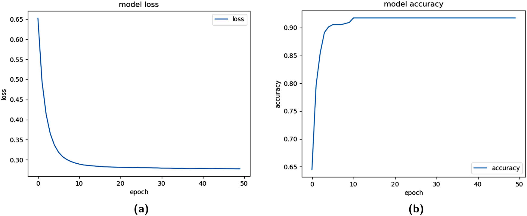
Training functions for fold=1 (Unbalanced dataset). (a) Training logloss plot and (b) training Acc plot.
5.3.2 Undersampling
In the undersampling scenario, all 46 case records were chosen, and 46 control records were chosen randomly from 506 records to match the total number of case records. Thus, 92 recordings were considered for the experiment. These 92 records were separated into a training split of 80%, a testing split of 20% of total records, and a validation split of 10% from the training split. The model underwent training with 200 epochs and 64 records per batch.
5.3.3 The weighted binary cross-entropy method
The imbalance in the dataset was addressed using the weighted binary cross-entropy approach. The weights were assigned to each class considering the proportion of 8.33% minority class vs 91.66% majority class. The weights resulted in one misclassification from the case category, contributing to as many as 11 misclassifications in the control category (considering 46 cases vs 506 controls in the dataset); the cross-fold method with 10 folds, a batch size of 64 examples. The 1D-CNN model was converged with 200 epochs during the training phase. The training logloss and Acc functions can be observed in Figure 5.
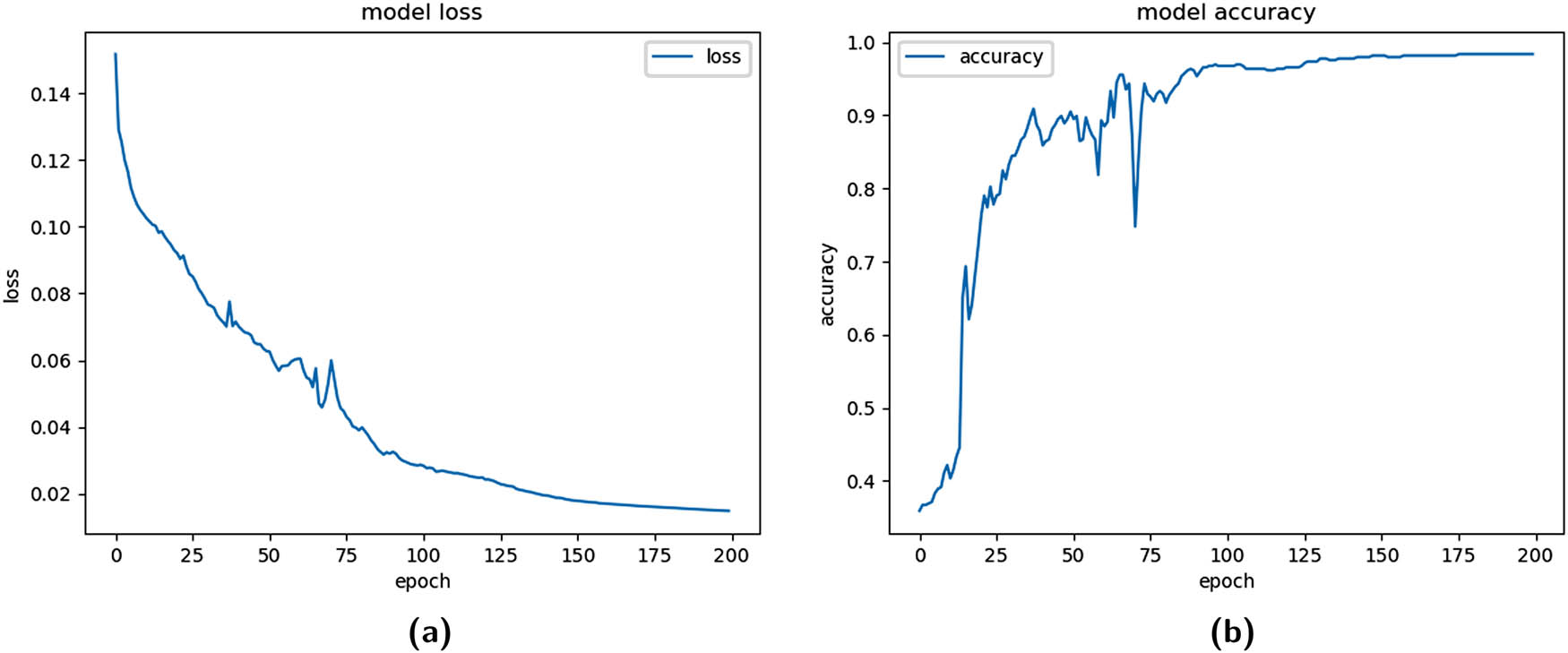
Training functions for fold = 1 (weighted binary cross-entropy). (a) Training logloss plot and (b) training Acc plot.
5.3.4 Oversampling using SMOTE
In the current approach, using SMOTE for oversampling, the minority class was made proportionate during the training phase. The cross-fold validation method was used with 10 folds, of which ninefolds were sent for SMOTE and then utilized for training, and onefold was preserved for testing. The model was empirically examined with different epoch values, and its performance was most remarkable for epoch 30, which is an outstanding accomplishment for the suggested model. The training logloss and Acc functions are illustrated in Figure 6.
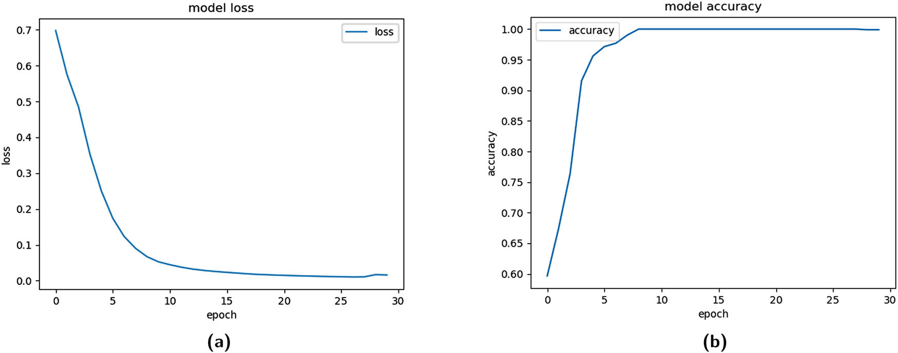
Training functions for fold = 1 (SMOTE). (a) Training logloss plot and (b) training Acc plot.
6 Results and discussion
The section enlists the results obtained in each data balancing approach. As discussed in Section 5, 31 simulations were carried out for each scenario, and the median (based on QI value) observation’s statistical parameters are reported here.
6.1 Unbalanced dataset
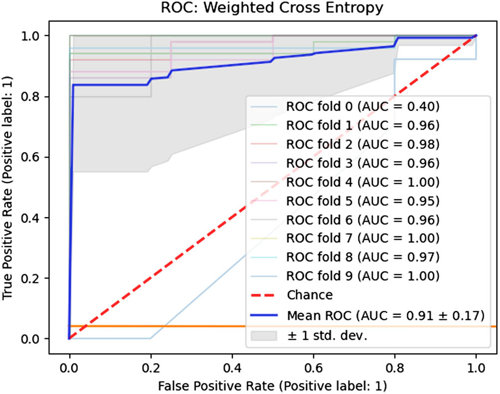
The unbalanced dataset was used as input for the 1D-CNN model, and Table 4 shows the various statistical parameters’ values during the training and testing phases. The median Se, Sp, and QI values were 0.9980, 0.1900, and 0.4355, whereas the AUC was 0.7140. The high value of Se shows that the model accurately detected cases of normal delivery, whereas low Sp suggests that cesarean section delivery cases were inadequately classified. The unbalanced data may be a contributing factor to this bias. The model demonstrated exceptional Acc, Pre, and F1-score performance during the test phase. Figure 7 shows the individual fold and overall mean AUC values.
1D-CNN model result for different class balance scenarios
| Phase | Loss | Acc | Pre | Se | Sp | QI | F1-Score | AUC |
|---|---|---|---|---|---|---|---|---|
| Unbalanced dataset | ||||||||
| Training (fold = 1) | 0.2774 | 0.9173 | 0.9173 | 1.00 | 0.00 | 0.00 | 0.9569 | 0.6027 |
| Training (fold = 10) | 0.1547 | 0.9517 | 0.9576 | 0.9912 | 0.5100 | 0.7125 | 0.9741 | 0.9058 |
| Testing | 0.2304 | 0.9312 | 0.9324 | 0.998 | 0.1900 | 0.4355 | 0.9641 | 0.7140 |
| Undersampling | ||||||||
| Training | 0.2119 | 0.9538 | 0.9429 | 0.9706 | 0.9355 | 0.9529 | 0.9565 | 0.9853 |
| Validation | 0.7354 | 0.50 | 0.5714 | 0.80 | 0.00 | 0.00 | 0.6666 | 0.30 |
| Testing | 0.8042 | 0.5263 | 0.4286 | 0.8571 | 0.3333 | 0.5345 | 0.5714 | 0.6667 |
| Weighted binary cross-entropy | ||||||||
| Training (fold = 1) | 0.0148 | 0.9839 | 0.9956 | 0.9868 | 0.9512 | 0.9688 | 0.9912 | 0.9967 |
| Training (fold = 10) | 0.0079 | 0.9940 | 1.00 | 0.9934 | 1.00 | 0.9967 | 0.9967 | 0.9953 |
| Testing | 0.2062 | 0.9458 | 0.9784 | 0.9625 | 0.7650 | 0.8581 | 0.9704 | 0.9180 |
| SMOTE | ||||||||
| Training (fold = 1) | 0.0601 | 0.9758 | 0.9656 | 0.9868 | 0.9648 | 0.9758 | 0.9761 | 0.9990 |
| Training (fold = 10) | 0.0003 | 1.00 | 1.00 | 1.00 | 1.00 | 1.00 | 1.00 | 1.00 |
| Testing | 0.0550 | 0.9875 | 0.9891 | 0.9981 | 0.8800 | 0.9372 | 0.9935 | 0.9510 |
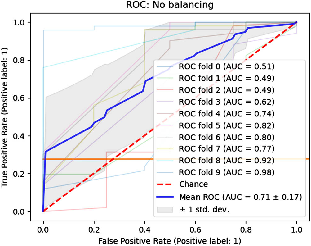
Fold-wise AUC values (unbalanced dataset).
6.2 Undersampling
The undersampling scenario considered 46 records from both classes. Table 4 lists the results for the undersampling example during the training, validation, and testing phases. This experiment produced low Se, Sp, QI, and AUC levels. The low results may be attributed to the small number of training instances used to build the model.
6.3 The weighted binary cross-entropy method
The weighted binary cross-entropy method resulted in boxplots for Se, Sp, and QI, as shown in the top row of Figure 8. The Se parameter ranged from 0.8757 (min) to 1.00 (max). The range of the Sp parameter was found to be 0.48 (min) to 0.9 (max). The low variance in the Se parameter suggests the model’s stability. The median Se, Sp, and QI are reported in Table 4 as 0.9625, 0.7650, and 0.8581, respectively. The Se value is adequate for identifying normal delivery records. The results obtained for the Sp and QI parameters are much better than those of the unbalanced dataset. Other metrics, such as Acc, Pre, and F1-Score, are also improved in the current scenario. Figure 9 provides the fold-wise AUC and mean AUC values.
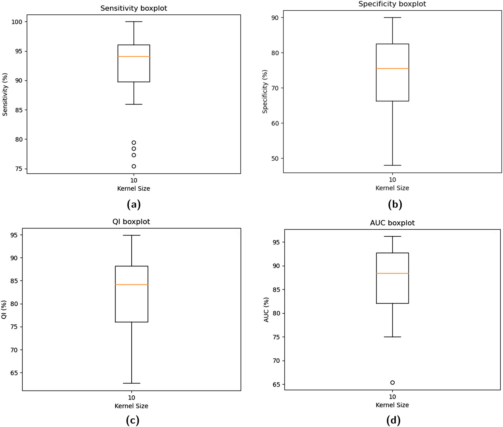
The boxplots for averaged performance parameters using
Fold-wise AUC values (weighted binary cross-entropy).
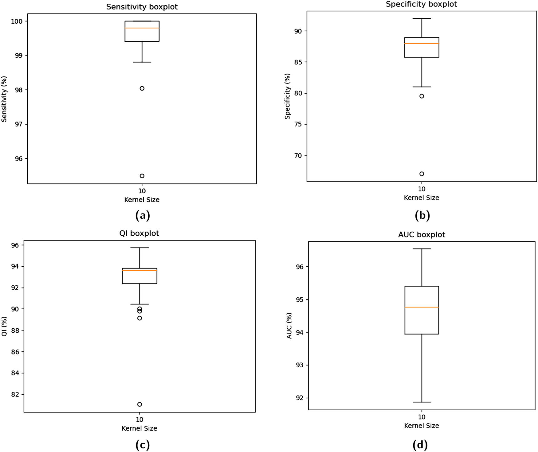
6.4 Oversampling using SMOTE
The SMOTE scenario used in the training phase resulted in Se, Sp, and QI boxplots, as represented by the bottom row in Figure 10. The range of Se parameter was 0.9881 (min) to 1.00 (max). The low variance from median to Q3 and zero variance from Q3 to max in the Se boxplot indicate a stable and consistent result. The range of the Sp parameter was found to be 0.81 (min)–0.92 (max). Once again, a low variance from the median to the Q3 value assures the model’s stability. The median Se value of 0.9981 and the Sp value of 0.88 are well balanced enough to discriminate between normal and cesarean sections, as supported by the outstanding QI of 0.9372 and AUC of 0.9510. The median values are represented in Table 4. Figure 11 depicts the fold-based and mean AUC values.
The boxplots for averaged performance parameters using
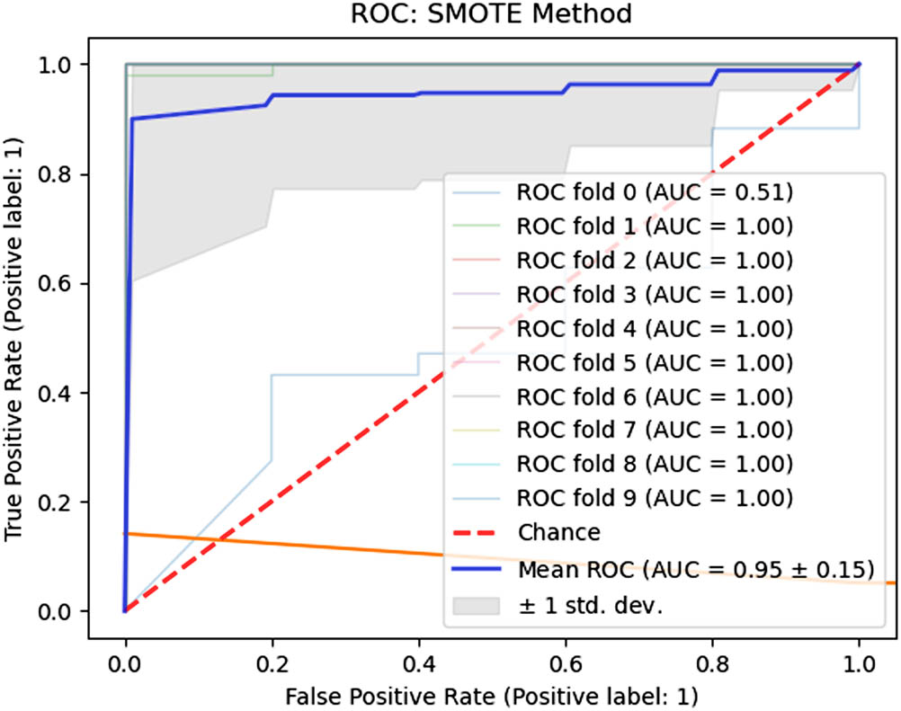
Fold-wise AUC values (SMOTE).
6.5 Comparison with existing literature
The findings of the suggested methodology are compared with the cutting-edge methods, with the CTU-UHB dataset serving as the fundamental criterion for the comparison. Table 5 summarizes the comparison’s results. The comparison uses the pertinent metrics Se, Sp, QI, and AUC. Case and control values are also mentioned since they influence the interpretation of the Se and Sp parameters. In the SMOTE oversampling situation, the Se and QI of the proposed technique are greater than those described in [17], while Sp is slightly lesser. In addition, complex engineering of features was required in [17]. Considering the scenario with weighted binary cross-entropy, the proposed approach has shown superior results than AUC [19] and [23]. Although Sp and AUC parameters in [21] are superior to the proposed method in the SMOTE scenario, Se is much better in the suggested method, and QI is almost equal to that in [21]. In addition, Saleem et al. [21] required complex feature engineering. Given the condition of an unbalanced dataset in [22] and the current work, the Se is still higher in this situation. Although [24] yielded better results regarding Sp, QI, and AUC, a few records from the CTU-UHB dataset were chosen for this study. In contrast, the present research used all available records, and Se is still performing better. The current analysis used a one-dimensional FHR signal, while a two-dimensional image generated from a one-dimensional FHR signal was used as input for the 2D-CNN method in [24]. The generation of two-dimensional images is an overhead and will require more computational power. In addition, one notable limitation when employing 2D-CNN is high computational requirements, which demand specialized hardware, especially for training. In this regard, 2D-CNN is not appropriate for applications that operate in real-time on mobile and low-power/low-memory devices [13]. All the parameters are higher in the proposed method than those in the study by Alsaggaf et al. [25] with the requirement of significant feature engineering. The segmentation approach was employed for class balancing in [27], and the current system’s performance utilizing the SMOTE scenario is superior for all assessment parameters. GAN addressed the imbalance in the dataset [28], but the suggested scheme excelled in all parameters.
Comparison with state-of-the-art
| Method | Data division criteria | Case and control value | Class balancing approach | Se (%) | Sp (%) | QI (%) | AUC (%) |
|---|---|---|---|---|---|---|---|
| Ensemble classifier (FLDA,RF,SVM) [17] | Type of delivery | Case:1 Control:0 | SMOTE | 87.00 | 90.00 | 88.49 | 96.00 |
| CNN [19] | pH value | Case:1 Control:0 | Weighted binary cross-entropy | — | — | — | 82.00 |
| AdaBoost [21] | Type of delivery | Case:0 Control:1 | SMOTE | 91.80 | 95.50 | 93.63 | 98.00 |
| SVM [22] | pH value | Case:1 Control:0 | — | 77.40 | 93.86 | 85.23 | 88.74 |
| MCNN and stacked MCNN [23] | pH value | Case:1 Control:0 | Weighted binary cross-entropy | — | — | — | 82.00 |
| CNN [24] | pH value | Case:0 Control:1 | Down sampling + image augmentation | 99.29 | 98.10 | 98.69 | 98.70 |
| SVM [25] | pH value, BDecf, Apgar score (1m & 5m) | Case:1 Control:0 | — | 74.29 | 99.55 | 86.00 | 89.30 |
| CNN [27] | Type of delivery | Case:0 Control:1 | Segmentation | 80.00 | 79.00 | 79.50 | 86.00 |
| CNN [28] | pH Value | Case:1 Control:0 | GAN data augmentation | 67.64 | 71.97 | 69.77 | — |
| Proposed method (1D-CNN) | Type of delivery | Case:0 Control:1 | 1. Unbalanced dataset | 99.80 | 19.00 | 43.55 | 71.40 |
| Type of delivery | Case:0 Control:1 | 2. Undersampling | 85.71 | 33.33 | 53.45 | 66.67 | |
| Type of delivery | Case:0 Control:1 | 3. Weighted binary cross-entropy | 96.25 | 76.50 | 85.81 | 91.80 | |
| Type of delivery | Case:0 Control:1 | 4. SMOTE | 99.81 | 88.00 | 93.72 | 95.10 |
6.6 Discussion
The CTG is an important fetal monitoring instrument during the intrapartum and antepartum phases. The CTG tracings are evaluated according to the FIGO criteria, yet inter-observer and intra-observer variability remains and may lead to unnecessary surgical births and cesarean sections. Recently, machine learning techniques have improved classification performance by reducing variance. An optimal set of input features, which remains challenging and time-consuming, influences the classification performance. The proposed model employed a 1D-CNN, suitable for a one-dimensional input, and has the notable trait of combining the feature mining and categorization methods in a single unit. The class balance is rarely present in medical datasets and is the second aspect influencing classification performance. The current study addresses the class imbalance problem using various scenarios: (i) considering the original unbalanced dataset; (ii) undersampling the dataset; (iii) employing the weighted binary cross-entropy method; and (iv) oversampling the dataset with SMOTE. The parameter tuning for the 1D-CNN model is done for two essential parameters: n_filters and kernel_s, as it highly impacts the overall performance of convolutional operation. The Se for the imbalanced dataset is 99.80%, which is an excellent classification rate for true positives (normal delivery cases) and suggests that unnecessary operational deliveries can be avoided. The bias introduced by an unbalanced dataset may account for a lower Sp value in this scenario. Due to the insufficient training examples, the outcome of the undersampling scenario needed improvement. During the weighted binary cross-entropy scenario, the 1D-CNN model performs significantly better than the unbalanced scenario, as Sp increases by 57.5%, QI by 42.26%, and AUC by 20.4%. However, a slight decrease in the Se by 3.55% can be observed here. The overall outcome due to the weighted cross-entropy method is significantly better than the unbalanced scenario. Compared to the weighted binary cross-entropy technique, SMOTE significantly increased around 11.5% in Sp, 7.91% in QI, 3.3% in AUC, and 3.56% in Se. Figure 12 shows a comparison graph of the four crucial parameters, Se, Sp, QI, and AUC, generated using four class balancing scenarios: unbalanced dataset, undersampling, weighted binary cross-entropy, and SMOTE. The graph demonstrates that the 1D-CNN model outperforms in terms of Sp, QI, and AUC in the SMOTE scenario compared to the rest.
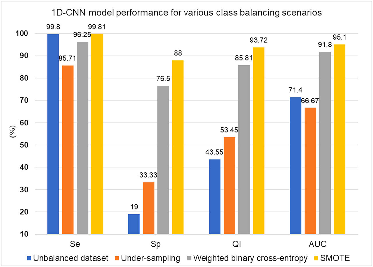
1D-CNN model performance under different class balance scenarios.
The boxplots for Se, Sp, QI, and AUC also mark stability and consistent performance due to the very low variance in the acceptable range during the SMOTE scenario, as shown in Figure 10.
The Se plays a crucial role in preventing unnecessary interventions during labor. Apart from undersampling, the suggested model is robust enough to demonstrate consistent Se in all circumstances. The Sp is a crucial metric as it helps avoid fetal compromise; hence, a rise in Sp in the SMOTE scenario is paramount. Although the Sp value in the training phase is relatively high in the SMOTE scenario due to the availability of oversampled case records, it dropped during the testing phase. The reason might be a smaller number of case records available during the testing phase. The learning rate decay and batch normalization method lead to early network convergence, ultimately lowering the number of training epochs in unbalanced and SMOTE conditions. This feature makes the proposed network worth using with portable devices, where less memory and power requirements must be satisfied. Second, the low computational requirement of the 1D-CNN model, without any additional overhead for input preparation during the testing phase, makes it suitable for real-time applications. The system’s stable and consistent performance may be due to correctly handling zero values in the FHR signal during the input normalization phase. The most crucial factor significantly impacting the overall performance is the proper selection of n_filters and kernel_s for the convolutional layer. After conducting many trials in each case, the authors carefully selected these values during fine-tuning experimentation. The fine-tuning of these values leads to satisfactory results regarding Se, Sp, QI, and AUC. The experiments for hyperparameter setting and layer-wise parameters also contributed to the overall results. However, the authors strongly feel that other deep learning methods combined with CNN might help increase overall predictive capability in SP, QI, and AUC values. The overall outcomes are promising for using this SMOTE method to avoid unnecessary cesarean sections and to detect fetal compromise. The comparison with the state-of-the-art methods is also encouraging toward the model’s usefulness in clinical practices.
7 Conclusion
The proposed framework automatically extracts features from an FHR signal using a 1D-CNN method. The experimentation employed a dataset with open access. The dataset was balanced using undersampling, weighted binary cross-entropy, and SMOTE methods. In all circumstances, besides undersampling, the sensitivity is very promising. The SMOTE scenario resulted in a Se of 99.81%, a Sp of 88%, a QI of 93.72%, and an AUC of 95.10%. Thus, the model has applicability in avoiding unnecessary cesarean sections and fetal compromise during the antepartum and intrapartum phases. In addition, the SMOTE scenario required a few epochs during the 1D-CNN training phase, significantly reducing training time. The proposed one-dimensional method is simple and does not require much input preparation compared to the two-dimensional model, and due to this lack of overhead, it will undoubtedly be helpful in real-time applications on portable low-memory/power devices.
In future work, we will evaluate the robustness of the suggested model using other datasets. In addition, different deep-learning variants adapted to time-series input can be used.
Acknowledgement
The authors thank the editor and referees for their insightful comments and suggestions.
-
Funding information: The authors state no funding involved.
-
Author contributions: Vidya Sujit Kurtadikar: conceptualization & design, methodology, software, validation, writing-original draft. Himangi Milind Pande: supervision, writing – reviewing and editing.
-
Conflict of interest: The authors state no conflicts of interest.
-
Data availability statement: The datasets analysed during the current study are available in the physionet repository, https://physionet.org/content/ctu-uhb-ctgdb/1.0.0/.
References
[1] Newborn Mortality. [homepage on the Internet]. Key facts, [updated 2022 January 28; cited 2023 April 02]. Available from: https://www.who.int/news-room/fact-sheets/detail/levels-and-trends-in-child-mortality-report-2021/.Suche in Google Scholar
[2] Ayres-de-Campos D, Spong CY, Chandraharan E. FIGO intrapartum fetal monitoring expert consensus panel. FIGO consensus guidelines on intrapartum fetal monitoring: Cardiotocography. Int J Gynaecol Obstet. 2015;131(1):13–24. 10.1016/j.ijgo.2015.06.020. Suche in Google Scholar PubMed
[3] NICE [homepage on the Internet]: Fetal monitoring in labour ∣ Guidance [updated 2022 December 14; cited 2023 April 02]. Available from: https://www.nice.org.uk/guidance/ng229/. Suche in Google Scholar
[4] Macones GA, Hankins GD, Spong CY, Hauth J, Moore T. The 2008 National Institute of Child Health and Human Development workshop report on electronic fetal monitoring: update on definitions, interpretation, and research guidelines. Obstetrics Gynecol. 2008;112(3):661–6. 10.1097/AOG.0b013e3181841395. Suche in Google Scholar PubMed
[5] Santo S, Ayres-de-Campos D, Costa-Santos C, Schnettler W, Ugwumadu A, Da Graça LM, et al. Agreement and accuracy using the FIGO, ACOG and NICE cardiotocography interpretation guidelines. Acta Obstetricia et Gynecologica Scandinavica. 2017;96(2):166–75. 10.1111/aogs.13064. Suche in Google Scholar PubMed
[6] Abdulhay EW, Oweis RJ, Alhaddad AM, Sublaban FN, Radwan MA, Almasaeed HM. Review article: non-invasive fetal heart rate monitoring techniques. Biomed Sci Eng. 2014;2(3):53–67. 10.12691/bse-2-3-2. Suche in Google Scholar
[7] Lobo Marques JA, Cortez PC, Madeiro JPDV, Fong SJ, Schlindwein FS, Albuquerque VHCD. Automatic cardiotocography diagnostic system based on Hilbert transform and adaptive threshold technique. IEEE Access. 2019;7:73085–94. 10.1109/ACCESS.2018.2877933. Suche in Google Scholar
[8] Ayres-de Campos D, Bernardes J, Garrido A, Marques-de-Sá J, Pereira-Leite L. SisPorto 2.0: a program for automated analysis of cardiotocograms. J Maternal-fetal Med. 2000;9(5):311–8. 10.1002/1520-6661(200009/10)9:5<311::AID-MFM12>3.0.CO;2-9. Suche in Google Scholar
[9] Pardey J, Moulden M, Redman CW. A computer system for the numerical analysis of nonstress tests. Amer J Obstetric Gynecol. 2002;186(5):1095–103. 10.1067/mob.2002.122447. Suche in Google Scholar
[10] Romano M, Bifulco P, Ruffo M, Improta G, Clemente F, Cesarelli M. Software for computerised analysis of cardiotocographic traces. Comput Meth Programs Biomed. 2016;124:121–37. 10.1016/j.cmpb.2015.10.008. Suche in Google Scholar
[11] Ayres-de-Campos D, Rei M, Nunes I, Sousa P, Bernardes J. SisPorto 4.0 - computer analysis following the 2015 FIGO Guidelines for intrapartum fetal monitoring. J Matern Fetal Neonatal Med. 2017;30(1):62–7. 10.3109/14767058.2016.1161750. Suche in Google Scholar
[12] Cömert Z, Kocamaz AF. Open-access software for analysis of fetal heart rate signals. Biomed Signal Process Control. 2018;45:98–108. 10.1016/j.bspc.2018.05.016. Suche in Google Scholar
[13] Kiranyaz S, Avci O, Abdeljaber O, Ince T, Gabbouj M, Inman DJ. 1D convolutional neural networks and applications: A survey, Mech Syst Signal Proces. 2021;151:107398. 10.1016/j.ymssp.2020.107398. Suche in Google Scholar
[14] Yılmaz E, Kılıkçıer C. Determination of fetal state from cardiotocogram using LS-SVM with particle swarm optimization and binary decision tree. Comput Math Meth Med. 2013;487179. 10.1155/2013/487179. Suche in Google Scholar PubMed PubMed Central
[15] Dash S, Quirk JG, Djurić PM. Fetal heart rate classification using generative models. IEEE Trans Biomed Eng. 2014;61(11):2796–805. 10.1109/TBME.2014.2330556. Suche in Google Scholar PubMed
[16] Spilka J, Frecon J, Leonarduzzi R, Pustelnik N, Abry P, Doret M. Sparse support vector machine for intrapartum fetal heart rate classification. IEEE J Biomed Health Inform. 2017;21(3):664–71. 10.1109/JBHI.2016.2546312. Suche in Google Scholar PubMed
[17] Fergus P, Selvaraj M, Chalmers C. Machine learning ensemble modelling to classify caesarean section and vaginal delivery types using Cardiotocography traces. Comput Biol Med. 2018;93:7–16. 10.1016/j.compbiomed.2017.12.002. Suche in Google Scholar PubMed
[18] Cömert Z, Kocamaz AF. Comparison of machine learning techniques for fetal heart rate classification. Acta Phys Polonica A. 2017;32:451–4. 10.12693/APhysPolA.132.451. Suche in Google Scholar
[19] Petrozziello A, Jordanov I, Aris Papageorghiou T, Christopher Redman WG, Georgieva A. Deep learning for continuous electronic fetal monitoring in labor. Annual International Conference of the IEEE Engineering in Medicine and Biology Society. IEEE Engineering in Medicine and Biology Society. Annual International Conference. 2018. p. 5866–9. 10.1109/EMBC.2018.8513625. Suche in Google Scholar PubMed
[20] Jianqiang L, Luxiang H, Zhixia S, Yifan Z, Min F, Bing L, et al. Automatic classification of fetal heart rate based on convolutional neural network. IEEE Internet Things J. 2019;6(2):1394–401. 10.1109/JIOT.2018.2845128. Suche in Google Scholar
[21] Saleem S, Naqvi SS, Manzoor T, Saeed A, Ur Rehman N, Mirza J. A strategy for classification of “Vaginal vs. Cesarean Section” delivery: Bivariate empirical mode decomposition of cardiotocographic recordings. Frontiers Physiol. 2019;10:246. 10.3389/fphys.2019.00246. Suche in Google Scholar PubMed PubMed Central
[22] Cömert Z, Şengür A, Budak Ü, Kocamaz AF. Prediction of intrapartum fetal hypoxia considering feature selection algorithms and machine learning models. Health Inform Sci Syst. 2019;7(1):17. 10.1007/s13755-019-0079-z. Suche in Google Scholar PubMed PubMed Central
[23] Petrozziello A, Redman CWG, Papageorghiou AT, Jordanov I, Georgieva A. Multimodal convolutional neural networks to detect fetal compromise during labor and delivery. IEEE Access. 2019;7:112026–36. 10.1109/ACCESS.2019.2933368. Suche in Google Scholar
[24] Zhao Z, Zhang Y, Comert Z, Deng Y. Computer-aided diagnosis system of fetal hypoxia incorporating recurrence plot with convolutional neural network. Front Physiol. 2019;10:255. 10.3389/fphys.2019.00255. Suche in Google Scholar PubMed PubMed Central
[25] Alsaggaf W, Cömert Z, Nour MK, Polat K, Brdesee HS, Toğaçar M. Predicting fetal hypoxia using common spatial pattern and machine learning from cardiotocography signals. Appl Acoustics. 2020;167:107429. 10.1016/j.apacoust.2020.107429. Suche in Google Scholar
[26] Subasi A, Kadasa B, Kremic E. Classification of the cardiotocogram data for anticipation of fetal risks using bagging ensemble classifier. Proc Comput Sci. 2020;168:34–9. 10.1016/j.procs.2020.02.248. Suche in Google Scholar
[27] Fergus P, Chalmers C, Montanez CC, Reilly D, Lisboa P, Pineles B. Modelling segmented cardiotocography time-series signals using one-dimensional convolutional neural networks for the early detection of abnormal birth outcomes. IEEE Trans Emerging Topics Comput Intelligence. 2021;5(6):882–92. 10.1109/TETCI.2020.3020061. Suche in Google Scholar
[28] Puspitasari RDI, Ma’sum M, Alhamidi MR, Kurnianingsih W, Jatmiko W. Generative adversarial networks for unbalanced fetal heart rate signal classification. ICT Express. 2022;8(2):239–43. 10.1016/j.icte.2021.06.007. Suche in Google Scholar
[29] LeCun Y, Bengio Y, Hinton G. Deep learning. Nature. 2015;521(7553):436–44. 10.1038/nature14539. Suche in Google Scholar PubMed
[30] Nie D, Trullo R, Lian J, Wang L, Petitjean C, Ruan S, et al. Medical image synthesis with deep convolutional adversarial networks. IEEE Trans Bio-med Eng. 2018;65(12):2720–30. 10.1109/TBME.2018.2814538. Suche in Google Scholar PubMed PubMed Central
[31] Chen TE, Yang SI, Ho LT, Tsai KH, Chen YH, Chang YF, et al. S1 and S2 heart sound recognition using deep neural networks. IEEE Trans Bio-med Eng. 2017;64(2):372–80. 10.1109/TBME.2016.2559800. Suche in Google Scholar PubMed
[32] Chudáček V, Spilka J, Burša M, Janků P, Hruban L, Huptych M, et al. Open access intrapartum CTG database. BMC Pregnancy Childbirth. 2014;14:16. 10.1186/1471-2393-14-16. Suche in Google Scholar PubMed PubMed Central
[33] Goldberger AL, Amaral LA, Glass L, Hausdorff JM, Ivanov PC, Mark RG, et al. PhysioBank, PhysioToolkit, and PhysioNet: components of a new research resource for complex physiologic signals. Circulation. 2000;101(23):E215–20. 10.1161/01.cir.101.23.e215. Suche in Google Scholar PubMed
[34] Chawla NV, Bowyer KW, Hall LO, Kegelmeyer WP. SMOTE: synthetic minority over-sampling technique. J Artif Intell Res. 2002;16:321–57. 10.1613/jair.953. Suche in Google Scholar
© 2024 the author(s), published by De Gruyter
This work is licensed under the Creative Commons Attribution 4.0 International License.
Artikel in diesem Heft
- Research Articles
- A study on intelligent translation of English sentences by a semantic feature extractor
- Detecting surface defects of heritage buildings based on deep learning
- Combining bag of visual words-based features with CNN in image classification
- Online addiction analysis and identification of students by applying gd-LSTM algorithm to educational behaviour data
- Improving multilayer perceptron neural network using two enhanced moth-flame optimizers to forecast iron ore prices
- Sentiment analysis model for cryptocurrency tweets using different deep learning techniques
- Periodic analysis of scenic spot passenger flow based on combination neural network prediction model
- Analysis of short-term wind speed variation, trends and prediction: A case study of Tamil Nadu, India
- Cloud computing-based framework for heart disease classification using quantum machine learning approach
- Research on teaching quality evaluation of higher vocational architecture majors based on enterprise platform with spherical fuzzy MAGDM
- Detection of sickle cell disease using deep neural networks and explainable artificial intelligence
- Interval-valued T-spherical fuzzy extended power aggregation operators and their application in multi-criteria decision-making
- Characterization of neighborhood operators based on neighborhood relationships
- Real-time pose estimation and motion tracking for motion performance using deep learning models
- QoS prediction using EMD-BiLSTM for II-IoT-secure communication systems
- A novel framework for single-valued neutrosophic MADM and applications to English-blended teaching quality evaluation
- An intelligent error correction model for English grammar with hybrid attention mechanism and RNN algorithm
- Prediction mechanism of depression tendency among college students under computer intelligent systems
- Research on grammatical error correction algorithm in English translation via deep learning
- Microblog sentiment analysis method using BTCBMA model in Spark big data environment
- Application and research of English composition tangent model based on unsupervised semantic space
- 1D-CNN: Classification of normal delivery and cesarean section types using cardiotocography time-series signals
- Real-time segmentation of short videos under VR technology in dynamic scenes
- Application of emotion recognition technology in psychological counseling for college students
- Classical music recommendation algorithm on art market audience expansion under deep learning
- A robust segmentation method combined with classification algorithms for field-based diagnosis of maize plant phytosanitary state
- Integration effect of artificial intelligence and traditional animation creation technology
- Artificial intelligence-driven education evaluation and scoring: Comparative exploration of machine learning algorithms
- Intelligent multiple-attributes decision support for classroom teaching quality evaluation in dance aesthetic education based on the GRA and information entropy
- A study on the application of multidimensional feature fusion attention mechanism based on sight detection and emotion recognition in online teaching
- Blockchain-enabled intelligent toll management system
- A multi-weapon detection using ensembled learning
- Deep and hand-crafted features based on Weierstrass elliptic function for MRI brain tumor classification
- Design of geometric flower pattern for clothing based on deep learning and interactive genetic algorithm
- Mathematical media art protection and paper-cut animation design under blockchain technology
- Deep reinforcement learning enhances artistic creativity: The case study of program art students integrating computer deep learning
- Transition from machine intelligence to knowledge intelligence: A multi-agent simulation approach to technology transfer
- Research on the TF–IDF algorithm combined with semantics for automatic extraction of keywords from network news texts
- Enhanced Jaya optimization for improving multilayer perceptron neural network in urban air quality prediction
- Design of visual symbol-aided system based on wireless network sensor and embedded system
- Construction of a mental health risk model for college students with long and short-term memory networks and early warning indicators
- Personalized resource recommendation method of student online learning platform based on LSTM and collaborative filtering
- Employment management system for universities based on improved decision tree
- English grammar intelligent error correction technology based on the n-gram language model
- Speech recognition and intelligent translation under multimodal human–computer interaction system
- Enhancing data security using Laplacian of Gaussian and Chacha20 encryption algorithm
- Construction of GCNN-based intelligent recommendation model for answering teachers in online learning system
- Neural network big data fusion in remote sensing image processing technology
- Research on the construction and reform path of online and offline mixed English teaching model in the internet era
- Real-time semantic segmentation based on BiSeNetV2 for wild road
- Online English writing teaching method that enhances teacher–student interaction
- Construction of a painting image classification model based on AI stroke feature extraction
- Big data analysis technology in regional economic market planning and enterprise market value prediction
- Location strategy for logistics distribution centers utilizing improved whale optimization algorithm
- Research on agricultural environmental monitoring Internet of Things based on edge computing and deep learning
- The application of curriculum recommendation algorithm in the driving mechanism of industry–teaching integration in colleges and universities under the background of education reform
- Application of online teaching-based classroom behavior capture and analysis system in student management
- Evaluation of online teaching quality in colleges and universities based on digital monitoring technology
- Face detection method based on improved YOLO-v4 network and attention mechanism
- Study on the current situation and influencing factors of corn import trade in China – based on the trade gravity model
- Research on business English grammar detection system based on LSTM model
- Multi-source auxiliary information tourist attraction and route recommendation algorithm based on graph attention network
- Multi-attribute perceptual fuzzy information decision-making technology in investment risk assessment of green finance Projects
- Research on image compression technology based on improved SPIHT compression algorithm for power grid data
- Optimal design of linear and nonlinear PID controllers for speed control of an electric vehicle
- Traditional landscape painting and art image restoration methods based on structural information guidance
- Traceability and analysis method for measurement laboratory testing data based on intelligent Internet of Things and deep belief network
- A speech-based convolutional neural network for human body posture classification
- The role of the O2O blended teaching model in improving the teaching effectiveness of physical education classes
- Genetic algorithm-assisted fuzzy clustering framework to solve resource-constrained project problems
- Behavior recognition algorithm based on a dual-stream residual convolutional neural network
- Ensemble learning and deep learning-based defect detection in power generation plants
- Optimal design of neural network-based fuzzy predictive control model for recommending educational resources in the context of information technology
- An artificial intelligence-enabled consumables tracking system for medical laboratories
- Utilization of deep learning in ideological and political education
- Detection of abnormal tourist behavior in scenic spots based on optimized Gaussian model for background modeling
- RGB-to-hyperspectral conversion for accessible melanoma detection: A CNN-based approach
- Optimization of the road bump and pothole detection technology using convolutional neural network
- Comparative analysis of impact of classification algorithms on security and performance bug reports
- Cross-dataset micro-expression identification based on facial ROIs contribution quantification
- Demystifying multiple sclerosis diagnosis using interpretable and understandable artificial intelligence
- Unifying optimization forces: Harnessing the fine-structure constant in an electromagnetic-gravity optimization framework
- E-commerce big data processing based on an improved RBF model
- Analysis of youth sports physical health data based on cloud computing and gait awareness
- CCLCap-AE-AVSS: Cycle consistency loss based capsule autoencoders for audio–visual speech synthesis
- An efficient node selection algorithm in the context of IoT-based vehicular ad hoc network for emergency service
- Computer aided diagnoses for detecting the severity of Keratoconus
- Improved rapidly exploring random tree using salp swarm algorithm
- Network security framework for Internet of medical things applications: A survey
- Predicting DoS and DDoS attacks in network security scenarios using a hybrid deep learning model
- Enhancing 5G communication in business networks with an innovative secured narrowband IoT framework
- Quokka swarm optimization: A new nature-inspired metaheuristic optimization algorithm
- Digital forensics architecture for real-time automated evidence collection and centralization: Leveraging security lake and modern data architecture
- Image modeling algorithm for environment design based on augmented and virtual reality technologies
- Enhancing IoT device security: CNN-SVM hybrid approach for real-time detection of DoS and DDoS attacks
- High-resolution image processing and entity recognition algorithm based on artificial intelligence
- Review Articles
- Transformative insights: Image-based breast cancer detection and severity assessment through advanced AI techniques
- Network and cybersecurity applications of defense in adversarial attacks: A state-of-the-art using machine learning and deep learning methods
- Applications of integrating artificial intelligence and big data: A comprehensive analysis
- A systematic review of symbiotic organisms search algorithm for data clustering and predictive analysis
- Modelling Bitcoin networks in terms of anonymity and privacy in the metaverse application within Industry 5.0: Comprehensive taxonomy, unsolved issues and suggested solution
- Systematic literature review on intrusion detection systems: Research trends, algorithms, methods, datasets, and limitations