Wheat freshness recognition leveraging Gramian angular field and attention-augmented resnet
-
Weiya Shi
 and
Liang Chen
and
Liang Chen

Abstract
During storage, wheat kernels undergo complex biochemical changes that affect their quality. Therefore, accurate and rapid measure of wheat freshness has immense economic and societal value. Using biophotonics and deep learning, this article explores the intricate relationship between wheat's ultra-weak bioluminescence signatures and its freshness. First, we select an advanced biophotonic system to capture time-varying bioluminescence data from kernels, which is then transformed into two-dimensional image styles employing the innovative Gramian angular field (GAF) method. Second, the image data serve as input to our proposed GAF-ResNet-GCT network architecture, which is specifically designed for wheat freshness classification and discrimination. The results underscore the effectiveness of our approach, demonstrating the model's remarkable ability to swiftly and precisely identify freshness with accuracy and robustness. The findings presented herein offer a groundbreaking scientific methodology for rapid, non-destructive wheat freshness detection, thereby advancing the application of biophotonics technology within the agricultural sector.
1 Introduction
With a booming global population and advances in the food industry, food security has become a top concern for governments and international organizations around the world. As a cornerstone food crop globally, wheat stands at the forefront of this discourse, with its yield and quality intimately tied to food security and the stability of national economies. During storage, wheat kernels inherently consume their own nutrients to sustain vital metabolic processes. However, with prolonged storage, the enzymatic activity within the grains gradually decreases or ceases, the respiration rates diminish, and the protoplasmic colloidal structure loses its compactness. The changes have a profound impact on the physical and chemical properties of wheat, leading to a deterioration in its edibility and processing performance.
As a crucial quality benchmark, the wheat kernel freshness encompasses both the duration of post-harvest storage and the subsequent series of quality changes that occur. Fresh wheat is typically superior quality, whereas prolonged storage can result in aged wheat, characterized by protein denaturation, elevated fatty acid levels, and alterations in chemical composition, all of which adversely affect the baking quality and flavor of the resulting flour. Consequently, accurate assessment of wheat freshness is of paramount practical significance, influencing key aspects of the grain procurement, storage, marketing, and processing chain.
Globally, the study of wheat freshness is a pivotal part of grain science research endeavors. Across international boundaries, a myriad of studies have delved into the physiological and biochemical variations in wheat and analyzed their impact on overall quality. Meanwhile, domestically, scholars have directed heightened attention toward exploring the intricate relationship between wheat freshness and its edible qualities.
Currently, the methods for identifying wheat freshness primarily encompass sensory evaluation and various biochemical approaches [1]. Sensory evaluation relies heavily on the subjective experience of the operator and is prone to interference from external factors, resulting in poor reproducibility. The evaluation results vary from person to person, making it suitable only as an auxiliary method. Physical tests such as the measurement of color and hardness are simple and easy to perform, but they lack accuracy. For example, Zhan et al. [2] conducted research on wheat freshness using thermal analysis techniques; Zhao et al. [3] used an electronic nose method to detect wheat of different origins and varieties, finding that this method also had a certain degree of effectiveness in identifying the origin and variety of wheat samples. Chemical analysis, such as the determination of protein content and fatty acid value, although more accurate, involves complex operations and is time-consuming. It generally requires complex pretreatment of the samples to be tested, and the various chemical reagents used in the detection process can cause certain environmental pollution. For example, He et al. [4] used the guaiacol method for rapid identification of wheat freshness; Yang et al. [5] applied the tetrazolium salt method to judge wheat freshness. These methods have certain limitations in practical applications, making it difficult to meet the demands of modern large-scale grain circulation. Therefore, the development of a rapid, accurate, and non-destructive technology for detecting wheat freshness has important practical needs in enhancing the efficiency and level of wheat quality management.
In recent years, some new testing technologies have been introduced into the study of wheat freshness. Liu et al. [6] used Fourier transform infrared spectroscopy to study wheat with different storage durations. The results showed that samples of the same variety produced in different years had similar spectra, but there were differences in the absorption intensity ratios, which increased with the extension of storage time. Wu et al. [7] applied near-infrared spectroscopy technology for non-destructive analysis of the changing trends of major chemical components during the short-term natural aging process of wheat seeds and combined with support vector machines to establish a rapid analytical model for discriminating the degree of natural aging of wheat seeds. Additionally, some studies [8] have utilized terahertz time-domain spectroscopy to test wheat samples stored for different years, obtaining optical parameters such as refractive index and absorption coefficient at specific wavelength bands. The results indicate that there are differences in the refractive index and absorption coefficient among wheat samples stored in different years, providing a novel experimental method for detecting and analyzing wheat freshness.
However, the above-mentioned detection methods all have certain limitations. Some require extensive manual intervention, which may compromise the objectivity of the detection results. Others lack a clear scientific correlation between the detection indicators and the characteristics, resulting in poor reproducibility of the results. Therefore, there is an urgent need to introduce new data sources and modern data analysis methods. Both theories and extensive practices have shown that wheat quality is essentially related to the activity and vitality of wheat grains. Consequently, the research approach can be shifted to exploring new information carriers of wheat's vital state and, based on this, investigating the degree of correlation between this information and its freshness. This serves as the starting point of this paper.
Inspired by the rapid development of biophotonic technology and deep learning, this research aims to integrate biophotonic analysis technology with modern signal processing and analysis theories. It seeks to explore, from a novel perspective, the mapping relationship between the freshness of wheat and the changing process of its biophotonic radiation state in order to develop a new, rapid, comprehensive, and non-destructive method for assessing wheat freshness. This research endeavors to broaden the application fields and research avenues of biophotonic analysis technology.
2 Related works
2.1 Biophotonics technology
Biophoton emission (BPE) pertains to the spontaneous emission of photons by biomolecules within living organisms during their transition from a higher to a lower energy state without the need for external stimuli. Although this emission is inherently feeble, modern photoelectric detection technologies are adept at capturing its subtle intensity. The spectral spectrum of BPE predominantly spans the 200–800 nm range, exhibiting a continuous distribution. Based on the presence or absence of external optical stimulation, BPE can be broadly classified into two categories: spontaneous bioluminescence and delayed bioluminescence. Amidst the relentless advancement of ultra-weak light detection technologies and profound investigations into biological information transmission, remarkable strides have been achieved in the realm of BPE research, as evidenced by studies [9,10].
In recent years, the burgeoning biophotonics technology has progressively garnered attention for its application in grain quality analysis. Wu et al. [11] conducted pioneering analytical research on the delayed luminescence characteristics of wheat samples, exploring variations across varieties and harvest years. Their findings underscored discernible differences in ultra-weak luminescence intensity, attributed to both production year and vitality within the same variety. Furthermore, Liang et al. [12] achieved remarkable precision in distinguishing four wheat varieties through the innovative integration of ultra-weak spontaneous light signals with power spectrum feature analysis. Previous investigations have consistently highlighted significant disparities in the spontaneous photon emission levels of wheat samples from diverse storage periods. Gong et al. [13,14], leveraging biophotonic instrumentation, conducted a meticulous study on the biophotonic signals of five wheat samples with varying storage histories. By incorporating an enhanced multi-scale permutation entropy algorithm for feature extraction from the photon signals, they revealed a compelling trend: the permutation entropy values of photon counts escalated with the prolongation of storage duration. This groundbreaking discovery furnishes empirical evidence for the efficacy of biophotonics in detecting wheat freshness, opening new avenues for quality assurance in the grain industry.
2.2 Feature extraction
Currently, the cornerstone of biophotonics research revolves around utilizing biophotonic testing equipment to accumulate photon emissions from experimental samples over time, generating one-dimensional time series data. This data primarily undergoes feature extraction in the statistical or frequency domains, subsequently leveraging diverse machine learning classification algorithms, such as support vector machines and BP neural networks, for discrimination. These methodologies fall under the umbrella of Time Series Classification (TSC), where time series data are arranged sequentially in time, capturing the dynamic changes within a system or process. TSC poses a pivotal yet intricate challenge in data mining, aimed at grouping time series data into distinct categories based on their inherent characteristics. To tackle this, researchers have devised a range of sophisticated techniques, including dynamic time warping [15], which aligns time series to measure their similarity; Bag-of-SFA Symbols [16], which captures local patterns; shapelet-based methods [17], which identify discriminatory subsequences; and Collective of Transformation Ensembles [18], an ensemble approach. Additionally, a multitude of machine learning algorithms [19] have been adapted to this domain, further enriching the TSC toolkit.
However, whether these extracted features are the most suitable for determining wheat quality and whether other more suitable features can be extracted from biophoton data remain to be seen. Most of these studies are still at the laboratory stage and have not yet formed a complete theoretical system or widely applied technical standards. In recent years, deep learning, as an important branch of artificial intelligence, is widely used in multiple fields such as image recognition, natural language processing, and speech recognition. Convolutional neural network (CNN) [20] is one of the most popular deep learning models, which, unlike traditional "feature-based" classification frameworks, do not require manual feature extraction. During the deep learning process, feature extraction involves automatically learning and identifying useful features from a large amount of data through multi-layer network structures, significantly enhancing the performance of models in various AI tasks. Their powerful feature extraction and pattern recognition capabilities enable them to perform excellently in processing one-dimensional time series data, such as electroencephalogram analysis [21], anomaly detection [22], etc.
Motivated by this inquiry, could the accumulated one-dimensional biophoton data potentially be transformed into two-dimensional images, facilitating further analysis via deep learning techniques? In the realm of mathematics, there exist proven methodologies for converting one-dimensional data into two-dimensional images, including but not limited to the relative position matrix [23], recurrence plot [24], Gramian angular field (GAF) [25,26], and Markov transition field [27]. These methods offer promising avenues for transforming our biophoton data into a format more amenable to deep learning-based processing and analysis.
In this study, we endeavor to transform the amassed wheat biophoton data into two-dimensional visual representations and subsequently leverage CNNs for feature extraction and classification, thereby validating the feasibility of differentiating wheat freshness utilizing biophotonic techniques. Initially, we collect biophoton data from wheat samples spanning multiple years and employ the GAF method to transform these temporal data into two-dimensional image data. Subsequently, we select the ResNet architecture as our primary network for feature extraction and classification tasks. To further refine classification performance, we integrate the Gaussian context transformer (GCT) attention mechanism, enhancing the network's ability to prioritize and learn from salient features within its layers. This approach aims to improve the accuracy and robustness of wheat freshness discrimination based on biophotonic analysis.
The main contributions of this article are summarized as follows:
Propose the adoption of biophotonic technology to address the method of distinguishing wheat freshness, thereby catalyzing the transition of this advanced technology from the confines of the laboratory into practical, real-world applications.
Innovatively propose the use of the GAF method to encode biophotonic data, transforming the original one-dimensional time-series data into two-dimensional data, with the pixels of the GAF image maintaining the correlation between the original time-series data.
Leveraging the residual network architecture and the attention mechanism, the GAF-ResNet-GCT network is proposed, a novel approach designed to amplify both the feature extraction capabilities and recognition performance of deep learning networks, ushering in a new era of enhanced accuracy and efficiency.
3 Materials and methods
To accurately discriminate wheat freshness, it is imperative to first acquire biophoton data from wheat samples spanning various years. This section delves into the experimental apparatus utilized, outlines the experimental protocol, and outlines the fundamental attributes of the gathered biophoton data. Then, the proposed GAF-ResNet-GCT architecture and implementation steps will be introduced.
3.1 The experimental equipment and configuration
This experiment employs the BPCL-ZL-TGC ultra-weak photon acquisition instrument as the primary measuring device, as depicted in Figure 1. The instrument is comprehensively designed, comprising four integral components: a measurement darkroom, collection equipment, signal analysis instruments, and a user-friendly front-end software interface. The measurement darkroom serves as the repository for test samples, ensuring optimal conditions for photon detection. The collection equipment, guided by software settings, diligently gathers the biophoton counts emanating from the samples within the darkroom. Subsequently, the signal analysis instruments meticulously process the collected data, performing essential analyses before seamlessly integrating the results into the intuitive front-end software for display, facilitating straightforward interpretation and analysis.
The BPCL-ZL-TGC ultra-weak photon acquisition instrument (taken by the author using a mobile phone in the school's food processing laboratory, permission and authorization have been obtained from the laboratory).
Prior to the measurement process, the samples underwent a rigorous pre-treatment phase within a darkroom for a duration of 30 min. This step was crucial in mitigating the disruptive effects of ambient light, ensuring the accuracy and reliability of the subsequent measurements. Environmental conditions were meticulously controlled, with an indoor temperature maintained at (28 ± 2)°C, a precise measurement temperature of (27.5 ± 0.5)°C, and an indoor humidity level kept within (45 ± 5)%. Furthermore, the test spectral wavelength range was set to encompass 380 to 620 nm, and the equipment operated at a standard voltage of 220 V, 50 Hz, ensuring optimal performance throughout the experimental procedure.
The wheat samples with storage years of 2020, 2021, 2022, and 2023 were collectively purchased from the local wheat seed market around October 2023. All relevant experimental work was initiated shortly after sample collection and completed between late 2023 and early 2024. Each precisely weighed sample (10.00 ± 0.02 g) underwent a 1,000-s measurement period, with biophoton counts meticulously recorded every second. Upon completion, we segmented the data from each experimental sample into ten equal parts, yielding a comprehensive dataset comprising 4,000 experimental samples, with 1,000 samples dedicated to each year.
Figure 2 distinctly showcases the temporal variation of photon counts for randomly selected wheat samples, spanning the years 2020–2023. The x-axis denotes time, while the y-axis represents the photon count, providing a clear visual representation of the dynamics. While these graphs exhibit characteristics akin to time series data, each year's sample data also possesses distinctive features, underscoring their uniqueness. Despite a discernible pattern in the data distribution, it is not immediately apparent which year's data corresponds to which graph. Therefore, to effectively distinguish between these samples, the implementation of feature extraction techniques and the application of classification algorithms becomes imperative.
Photon counts for wheat samples from each year from 2020 to 2023.
The determination of specific features to extract from the data often lacks a definitive criterion. Traditional approaches encompass the extraction of statistical features (e.g., mean, variance) and the transformation of time-series data into the frequency domain through techniques like Fourier transform and wavelet transform. However, this article innovatively harnesses the power of deep learning, which circumvents the manual selection of features by enabling the autonomous discovery of discriminative characteristics. To this end, we employ the GAF methodology, transforming one-dimensional time-series data into two-dimensional image data. This transformation facilitates the utilization of deep learning algorithms, which can then learn and extract the distinguishing features in an automated fashion.
3.2 Related concepts of GAF representation
The GAF is a method that converts one-dimensional time-series data into two-dimensional images. The core of the GAF method lies in pairing the data points in the time series, calculating the cosine of the angle between them, and representing these calculations as pixel values in an image. This method can effectively capture the dynamic and periodic characteristics of time-series data, preserving the complete information and temporal dependencies of the time series. Specifically, the GAF encompasses two forms: the Gramian angular summation field (GASF) and the Gramian angular difference field (GADF). GASF generates an image by calculating the cosine of the sum of angles between each pair of time series values in a polar coordinate system, while GADF generates an image by calculating the sine of the difference in angles.
The implementation of the GAF typically involves the following steps:
Preprocessing and normalization: Preprocess the raw time series data by normalizing it to a specific interval (e.g., [0, 1] or (−1, 1)) to eliminate potential impacts from different scales on the results. This is typically achieved using the min–max normalization method. Assuming there is a time series
(1)Constructing the Gram matrix: Treat each data point in the time series as a vector in a high-dimensional space and compute the inner product between these vectors to form the so-called Gram matrix. Each element of this matrix represents the similarity between two data points. The Gram matrix is expressed as shown in formula (2):
(2)where each element is the inner product of two time series data points, as shown in formula (3):
(3)As the elements in the Gram matrix follow a Gaussian distribution centered at 0, it is difficult to distinguish its information from Gaussian noise. Moreover, since univariate time series are one-dimensional, the dot product cannot differentiate between valuable information and Gaussian noise, thus necessitating a change in space. Inspired by polar coordinate transformation, we will construct a bijective mapping between the one-dimensional time series and a two-dimensional space, mapping the preprocessed time series values into a polar coordinate system, where the timestamps serve as the radii, and the scaled values are converted into angles through the inverse cosine function. The transformation formula is as follows:
(4)(5)where
As any operation analogous to an inner product inevitably combines the information from two different observations into a single value, the following definitions are typically used for performing inner product calculations. This enables better preservation of the complete information and temporal dependencies within the time series, ensuring no information is lost
(6)Generate GAF image: Based on the definitions of GASF or GADF mentioned above, the cosine or sine values of the angles for each pair of values in the polar coordinate system can be calculated to generate a two-dimensional image
Figure 3 presents the GASF and GADF images corresponding to the wheat biophoton data for different years shown in Figure 2.
The GASF and GADF images corresponding to biophoton data shown in Figure 2.
The advantage of the GAF approach lies in its unique ability to seamlessly integrate temporal information from time-series data with the prowess of deep learning algorithms, which have garnered immense popularity in image processing. This fusion not only elevates the efficiency of feature extraction but also streamlines the entire data analysis process. By converting one-dimensional time-series data into two-dimensional image representations, GAF paves the way for the application of advanced deep learning techniques, thereby simplifying and enhancing the analysis.
3.3 ResNet
CNNs are widely utilized models in deep learning, characterized by their core features of local connectivity, parameter sharing, and automatic feature extraction. Despite CNNs' powerful feature extraction capabilities, they still face challenges when dealing with extremely deep networks. As the number of network layers increases, the training error tends to gradually decrease and reach saturation, but then as the number of layers further increases, the training error rises again, manifesting as the so-called degradation problem. The emergence of ResNet [28] effectively addresses this issue by introducing shortcut connections, which not only ensures the depth of the network but also optimizes gradient propagation, making the network easier to train and converge. This is of great significance for complex tasks in practical applications, such as high-precision image classification and large-scale image processing.
Specifically, the residual block in ResNet comprises two paths: one is the path for normal convolution operations, which typically begins with a convolution layer, followed by a batch normalization layer and a ReLU activation function. This combination helps reduce internal covariate shifts and accelerates the training process. The ReLU activation function adds nonlinearity, enabling the network to learn more complex patterns, followed by another convolution operation and batch normalization. The other path is an identity mapping path. As shown in Figure 4, finally, the outputs of these two paths are added together to form the final output of the residual block. This output is then activated by a ReLU activation function, generating the final output feature of the residual block.
Residual block in ResNet.
As illustrated in the Figure 4, x represents the input, and F(x) denotes the output of the residual block before the second activation function. The core formula of the residual block can be expressed as
This design has two key advantages: First, it simplifies the learning process because instead of learning a complete output, it learns a residual mapping. Second, it provides a shortcut that allows skipping some layers, alleviating the problem of gradient vanishing, enabling deeper networks to be effectively trained. The residual blocks in ResNet are mainly classified into two types: basic residual blocks and bottleneck residual blocks. A basic residual block consists of two 3 × 3 convolutional layers, each followed by a batch normalization layer and a ReLU activation function. The input passes through these convolutional layers and is then added to the original input, before being output through a ReLU activation function. The bottleneck residual block contains three convolutional layers: The first 1 × 1 convolutional layer is used to reduce the number of channels, followed by a 3 × 3 convolutional layer, and finally, another 1 × 1 convolutional layer to restore the original number of channels. This design reduces computational complexity while retaining sufficient information.
3.4 GCT attention module
The primary role of introducing attention mechanisms into CNN is to enhance the model's ability to focus on critical information within the input data, thereby improving the model's performance and efficiency, such as the channel attention mechanism SE [29]. However, literature [30] points out that the SE module tends to learn a negative correlation between features, meaning that when the difference between the global context and the average value increases, the obtained attention excitation value will correspondingly decrease. Based on this correlation, literature [31] proposes GCT for modeling global context, where GCT can directly replace the two fully connected layers in SE with a Gaussian function that incorporates negative correlation. Compared to SE, GCT is able to better learn the negative correlation between global context and attention activation values with fewer introduced parameters, thereby enhancing the model's expressive power.
The basic structure of GCT is illustrated in Figure 5. GCT comprises three parts: GCA (global context aggregation), normalization, and Gaussian context excitation. Specifically, a feature map of dimension
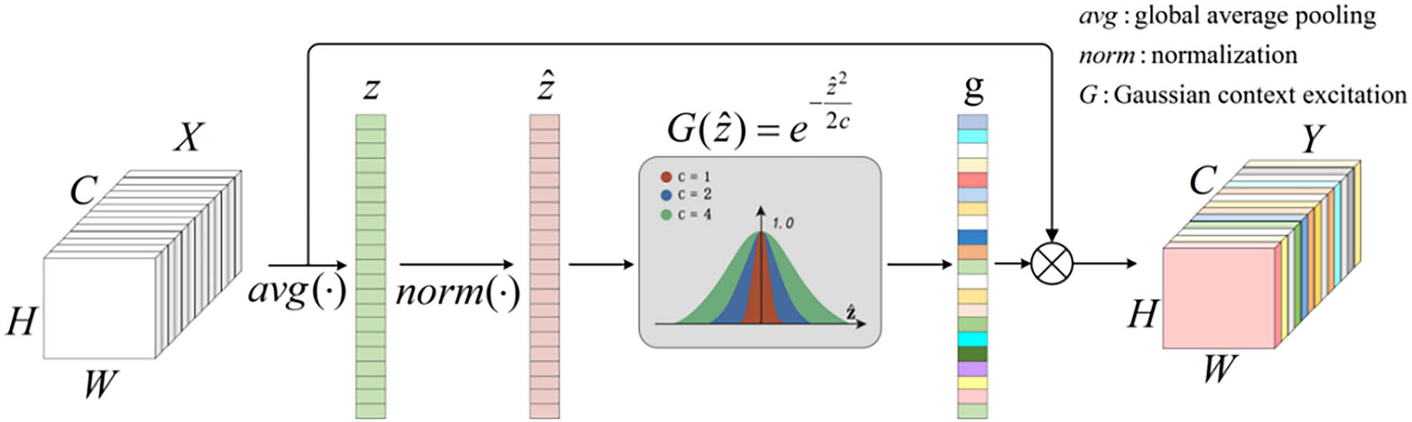
Schematic diagram of the GCT network structure.
In the equation, C denotes the number of channels, while H and W represent the width and height of the feature map, respectively. Afterwards, z undergoes feature normalization using the function norm(), as shown in the following equation:
In the equation,
The normalized result
Combining all the above operations into a single equation, we construct the GCT module, as shown in the following equation:
3.5 Proposed GAF-Resnet-GCT network
This article proposes the integration of the GCT attention mechanism within residual blocks, constituting a novel architecture dubbed the GAF-ResNet-GCT network. This attention mechanism augments ResNet's capabilities by enabling it to autonomously discern and extract more discriminative features across various levels, dynamically learn optimal feature weights, and subsequently adjust the significance of features across channels. As a result, the representational prowess of the network is significantly bolstered. The diagram of the network structure is shown in Figure 6.
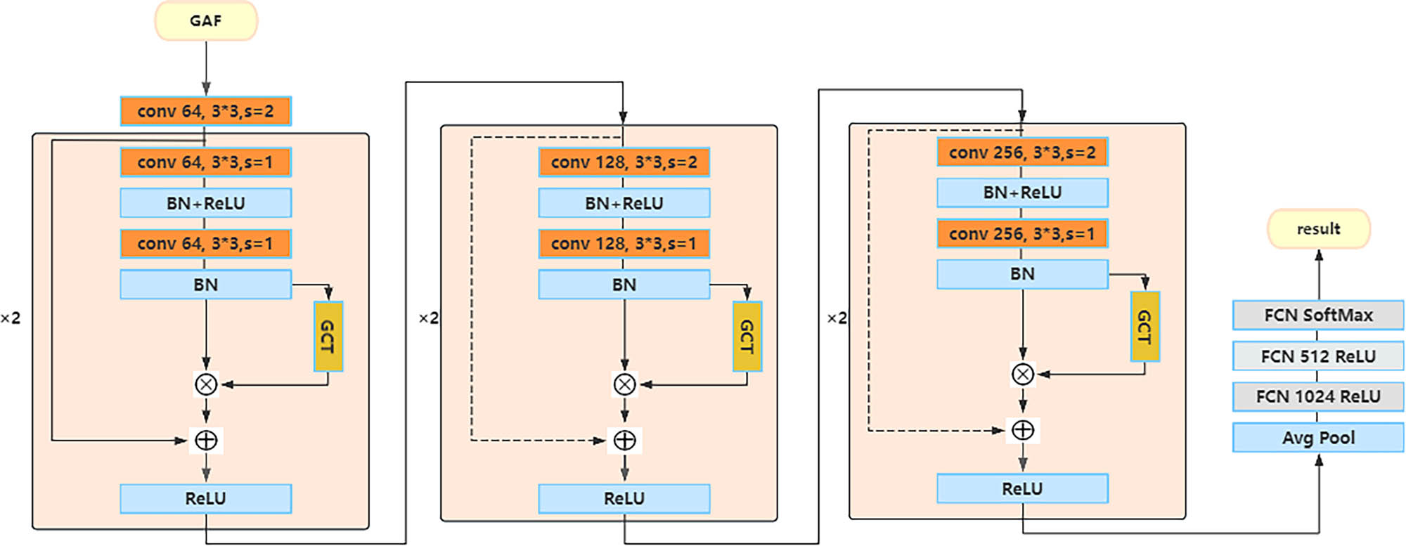
The diagram of the proposed GAF-Resnet-GCT network structure.
The entire network architecture consists of six residual blocks. The GAF image is initially passed through a standard convolutional layer for extracting initial features, followed by six residual blocks. In the third and fifth residual blocks, the first convolution halves the input image size and doubles the number of channels; hence, a 1 × 1 convolution is used to implement the shortcut connection. All other connections use identity mappings directly. Within the residual blocks, batch normalization and the ReLU function are applied after the convolutional layers. In the output stage, global average pooling is used to adjust the multi-channel data into a one-dimensional format, which is then connected to three fully connected layers. The numbers of neurons in these fully connected layers are 1,024, 512, and the number of classification categories (four categories in this experiment), respectively. The middle fully connected layer uses the ReLU activation function, while the final layer employs the SoftMax function to calculate the maximum probability value. In the residual module, the GCTmodule receives the feature map from the previous layer as input and generates a channel attention weight matrix through an attention layer. This weight matrix is then used to perform a weighted summation on the input feature map, resulting in a feature map that contains global context information. This process not only enhances the spatial representation capabilities of the features but also enables the network to focus on the information regions that are more critical to the task.
3.6 Diagnostic procedure of proposed method
Figure 7 illustrates the diagnostic procedure of the proposed GAF-Resnet-GCT.

The diagnostic process of the proposed GAF-Resnet-GCT. Source: Created by the authors.
The detailed procedures for freshness diagnosis are as follows:
To collect photon data from wheat samples spanning multiple years using a BPCL-ZL-TGC ultra-weak photon system
To transform biophoton data into two-dimensional images used GAF.
Construct the GAF-Resnet-GCT model, configure the network hyperparameters such as learning rate, the number of training iterations, and initialize the network weights.
The GAF-Resnet-GCT is trained utilizing the samples from the training set, and the deviation between the network's output and the sample labels is computed utilizing the cross-entropy loss function. This error is then propagated back through the network according to the Adam gradient descent algorithm, leading to an update of the network's weight parameters. The network's performance is assessed using the validation set after each training iteration; however, error backpropagation and updates to the network weights are not executed during this evaluation phase.
The fully trained GAF-Resnet-GCT is employed to evaluate the test set and provide the ultimate diagnostic outcome.
3.7 Evaluation metrics
Accurately assessing the performance of a model is crucial. To ensure a comprehensive evaluation of the model, this article adopts Accuracy, Precision, Recall, and F1 Score as key indicators to evaluate the model's performance. Each of these metrics reflects the model's performance from different angles, complementing each other and collectively providing a comprehensive measurement standard for model evaluation. Their calculation formulas are as follows:
where TP, FP, FN, and TN, respectively, represent the number of true positives, false positives, false negatives, and true negatives.
4 Results and discussions
To facilitate model training and evaluation, we partitioned the experimental data into training, validation, and test sets in an 8:1:1 ratio and employed a rigorous 10-fold cross-validation approach to ensure the accuracy and reliability of our experimental results.
The NVIDIA GeForce GTX 4090d graphics card was utilized for model training, ensuring high-performance computational capabilities. The training process was configured with a batch size of 32, optimized using the Adam algorithm, which is renowned for its efficiency in gradient descent optimization. To enhance generalization and prevent overfitting, a Dropout parameter of 0.5 was employed, alongside an initial learning rate of 1 × 10⁻³. After every ten steps of model updates, a rigorous evaluation was conducted on the validation set to identify the optimal weight configuration that yields the highest accuracy, thus safeguarding against overfitting to the training data.
4.1 Comparative experiments with other methods
To rigorously evaluate the efficacy of our proposed algorithm, we selected a diverse array of deep learning algorithms (CNN, ResNet) and traditional machine learning algorithms (KNN, SVM, BP) as benchmarks for classification performance comparison. Notably, traditional machine learning approaches necessitate manual feature selection, which encompassed six statistical features: median, mean, quartile deviation, mean deviation, variance, and coefficient of variance in this study. This comprehensive evaluation framework allowed us to assess the strengths and limitations of our algorithm in comparison to both modern deep learning and established machine learning techniques. Table 1 presents the experimental results.
Experimental results using different methods
| KNN | SVM | BP | CNN | ResNet | GAF-ResNet-GCT | |
|---|---|---|---|---|---|---|
| Accuracy | 0.816 ± 0.014 | 0.872 ± 0.020 | 0.892 ± 0.016 | 0.912 ± 0.009 | 0.918 ± 0.007 | 0.931 ± 0.011 |
| Precision | 0.817 ± 0.015 | 0.873 ± 0.021 | 0.894 ± 0.016 | 0.914 ± 0.009 | 0.920 ± 0.007 | 0.933 ± 0.010 |
| Recall | 0.816 ± 0.015 | 0.872 ± 0.020 | 0.892 ± 0.016 | 0.912 ± 0.009 | 0.918 ± 0.007 | 0.931 ± 0.011 |
| F1 score | 0.816 ± 0.014 | 0.872 ± 0.021 | 0.892 ± 0.016 | 0.912 ± 0.009 | 0.918 ± 0.007 | 0.931 ± 0.011 |
The table reveals that among the three traditional methods – KNN, SVM, and BP – the accuracy rates stand at 81.6, 87.2, and 89.2%, respectively, with their precision, recall, and F1 scores demonstrating relative parity. Notably, the BP algorithm and SVM algorithm outshine in classification performance. These methods rely on six manually selected statistical features as inputs into various machine learning algorithms. Nevertheless, the manual selection of features from the biophotonic time-series data, lacking optimality, limits the optimality of classification results. Consequently, there remains a pressing need for feature optimization through diverse methodologies to further enhance performance.
Both CNN and ResNet, rooted in deep learning algorithms, eliminate the dependency on manual feature selection by enabling the network to learn autonomously. The accuracy rates of these two methods stand at 91.2 and 91.8%, respectively, with ResNet marginally surpassing CNN due to its innovative use of residual structures. These structures facilitate more efficient updates and iterations of network weights, contributing to slightly higher accuracy. Notably, even with a moderately deep network architecture in this experiment, the effectiveness of both methods is expected to escalate with an increase in the number of layers. Furthermore, this study validates the feasibility of transforming one-dimensional biophotonic data into two-dimensional GAF graphs and subsequently leveraging deep learning for feature extraction and classification, underscoring the potential of this proposed approach.
Upon integrating the attention mechanism GCT, the GAF-ResNet-GCT network achieved a notable improvement in accuracy, reaching 93.1%, marking a 1.3% increase over the baseline ResNet model. This enhancement underscores the power of the attention mechanism in enhancing the network's ability to prioritize key features and elevate classification precision, ultimately translating into higher classification accuracy. Moreover, this achievement underscores the significant potential of incorporating attention mechanisms into deep learning frameworks, as proposed in this article, to bolster overall performance. To make the results clearer, Figure 8 presents bar charts corresponding to the results of different algorithms in Table 1.
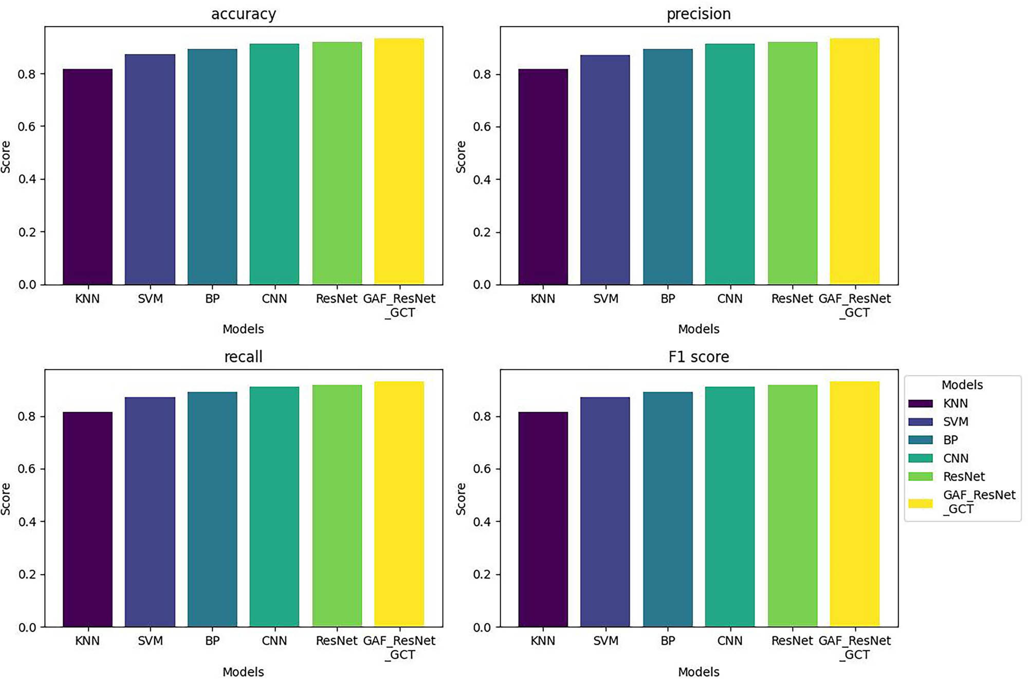
Experimental results using different methods.
4.2 Comparative experiment between GASF and GADF
To assess the impact of the two GAF methods – GASF and GADF – on experimental outcomes, additional experiments have been conducted. While previous tests employed GASF, the hyperparameters utilized in this section mirror those for training GASF images, ensuring a fair comparison. Table 2 summarizes the results. Initially, employing GADF to generate the two-dimensional matrix and inputting it into the proposed network revealed a notable improvement in accuracy, reaching 94.3%, a 1.3% increase over GASF. A closer examination of the two-dimensional graphs from Figure 3 reveals that GADF outperforms GASF in color intensity, detail rendering, and line proportion, contributing to its superior detection accuracy. Furthermore, an intriguing discovery was made when both GASF and GADF-generated graphs were shuffled and fed into the network: the accuracy climbed even higher to 94.5%, suggesting a slight yet significant enhancement over exclusive GADF use, demonstrating the potential of combining both methods.
Experimental results using GASF and GADF
| GASF | GADF | GASF+GADF | |
|---|---|---|---|
| Accuracy | 0.931 ± 0.011 | 0.943 ± 0.013 | 0.945 ± 0.016 |
| Precision | 0.933 ± 0.010 | 0.944 ± 0.014 | 0.947 ± 0.017 |
| Recall | 0.931 ± 0.011 | 0.943 ± 0.013 | 0.945 ± 0.016 |
| F1 score | 0.931 ± 0.011 | 0.943 ± 0.013 | 0.945 ± 0.016 |
4.3 Confusion matrix for classification results
Figure 9 illustrates the confusion matrices for the final classifications achieved using GDSF-ResNet-GCT and the BP network for comparative purposes. Analyzing the GDSF-ResNet-GCT matrix, we observe a marked improvement in accuracy, with just three misclassifications in 2020, two in 2021, and two in 2022, whereas all samples from 2023 were correctly identified. This heightened recognition accuracy hints at enhanced internal biological activity and more robust BPE in the newer wheat seeds. Conversely, the BP method's matrix reveals a higher degree of misclassification, with four errors in 2020, four in 2021, three in 2022, and two in 2023, underscoring the reduced freshness and weaker biometric signals emanating from older wheat samples compared to their fresher counterparts.
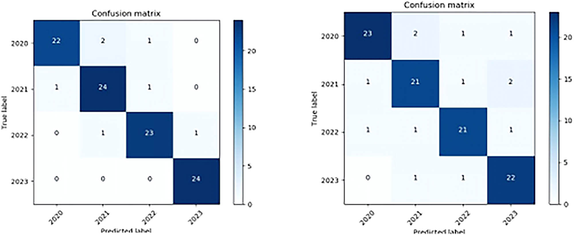
Confusion matrix.
5 Conclusion
This article presents the innovative application of biophotonics and deep learning technology to assess the freshness of wheat. The methodology involves transforming the collected one-dimensional time series data into two-dimensional image data through the GAF method, followed by the employment of a deep learning approach to autonomously identify salient features. To boost algorithm speed and efficiency, the GAF-ResNet-GCT network architecture is introduced, which attention mechanism is introduced to focus on important features. Experimental outcomes conclusively demonstrate the superiority of the proposed method over the existing ones in terms of classification accuracy.
Moreover, this work introduces a fresh perspective and methodology for wheat freshness classification, highlighting the potential of biophotonics in revealing intricate cellular and molecular alterations during wheat storage. This insight provides a solid scientific foundation for optimizing storage conditions and prolonging wheat shelf life, presenting promising avenues for future research endeavors.
Acknowledgments
The work is supported by High Performance Computing Platform of Henan University of Technology.
-
Funding information: This work was supported in part by the National Natural Science Foundation of China under Grant 62006071, part by the Science and Technology Research Project of Henan Province under Grant 232103810086, and part by Henan University of Technology Grain Information Processing Center Open Fund under Grant KFJJ2023010.
-
Author contributions: All authors have accepted responsibility for the entire content of this manuscript and consented to its submission to the journal, reviewed all the results and approved the final version of the manuscript. WS: methodology, original draft preparation, reviewing and editing, and final drafting. LC: programming, validation, writing, reviewing, and editing.
-
Conflict of interest: Authors state no conflict of interest.
-
Data availability statement: The datasets generated during and/or analysed during the current study are available from the corresponding author on reasonable request.
References
[1] Zhang HH, Wu XL, Qi M, Tang HL, Ye FK. Analysis of the current status and exploration of new methods for identifying the freshness of wheat. Grain Process. 2016;41(3):17–20.Search in Google Scholar
[2] Zhan HJ, Fan L, Zhou ZM. Research on evaluating wheat freshness using thermal analysis techniques. J Chin Cereals Oils Assoc. 2003;18(1):78–80.Search in Google Scholar
[3] Zhao D, Zhang YR, Lin JY. Application of electronic nose in quality control of wheat. Cereal Feed Ind. 2012;(3):10–5.Search in Google Scholar
[4] He XC, Guo DL, Feng YJ. Research on rapid identification methods for freshness of wheat. Grain Storage. 2006;(1):42–5.Search in Google Scholar
[5] Yang HP, Song W, Yuan J. Preliminary exploration of methods for identifying wheat aging degree. J Chin Cereals Oils Assoc. 2004;19(6):23–6.Search in Google Scholar
[6] Liu F, Li T, Liu G. Infrared spectroscopy study of wheat and red beans stored for different years. J Light Scattering. 2010;22(6):186–9.Search in Google Scholar
[7] Wu JZ, Li H, Zhang HD, Mao WH, Liu CL, Sun XR. Non-destructive identification of natural aging degree of wheat seeds using near-infrared spectroscopy. Spectrosc Spectr Anal. 2019;39(3):751–5.Search in Google Scholar
[8] Ge HY, Jiang YY, Ma HH. Research on THz rapid non-destructive detection of wheat freshness. J Light Scattering. 2015;27(6):191–4.Search in Google Scholar
[9] Chen S, Huang CY, Moran L. Biological ultra-weak luminescence and its applications. J Huangshi Inst Technol. 2006;22(4):82–4.Search in Google Scholar
[10] Yoshinaga N, Kato K, Kageyama C. Ultraweak photon emission from herbivory-injured maize plants. Die Naturwissenschaften. 2006;93(1):38–41.10.1007/s00114-005-0059-9Search in Google Scholar PubMed
[11] Wu CZ, Niu QF, Zhang LJ. Research on the detection method of wheat vitality based on ultra-weak delayed luminescence. J Chin Cereals Oils Assoc. 2015;30(6):121–4.Search in Google Scholar
[12] Liang YT, Song HX, Liu Q. Study on spectrum estimation in biophoton emission signal analysis of wheat varieties. Math Probl Eng. 2014;2014(2):1–9.10.1155/2014/606275Search in Google Scholar
[13] Gong YH, Yang TJ, Liang YT. Integrating ultraweak luminescence properties and multi-scale permutation entropy algorithm to analyze freshness degree of wheat kernel. Optik. 2020;218(9):1–8.10.1016/j.ijleo.2020.165099Search in Google Scholar
[14] Gong YH, Yang TJ, Liang YT. Rapid nondestructive detection of wheat freshness based on biophotonics. Spectrosc Spectr Anal. 2021;41(7):2166–70.Search in Google Scholar
[15] Rakthanmanon T, Campana B, Mueen A. Searching and mining trillions of time series subsequences under dynamic time warping. Acm Sigkdd International Conference on Knowledge Discovery & Data Mining. ACM; 2012.10.1145/2339530.2339576Search in Google Scholar PubMed PubMed Central
[16] Schfer P. The boss is concerned with time series classification in the presence of noise. Data Min Knowl Discov. 2015;29(6):1505–30.10.1007/s10618-014-0377-7Search in Google Scholar
[17] Ye L, Keogh EJ. Time series shapelets: A new primitive for data mining. Acm Sigkdd International Conference on Knowledge Discovery & Data Mining. ACM; 2009.10.1145/1557019.1557122Search in Google Scholar
[18] Bagnall A, Lines J, Hills J. Time-series classification with cote: the collective of transformation-based ensembles. IEEE Trans Knowl Data Eng. 2015;27(9):2522–35.10.1109/TKDE.2015.2416723Search in Google Scholar
[19] Zhang WN, Zhao HY, Yu Y. Hands on machine learning. Beijing: People’s Telecom Publishing House; 2023.Search in Google Scholar
[20] LeCun Y, Bengio Y, Hinton G. Deep learning. Nature. 2015;521:436–44.10.1038/nature14539Search in Google Scholar PubMed
[21] Li G, Li J, Ju Z, Sun Y, Kong J. A novel feature extraction method for machine learning based on surface electromyography from healthy brain. Neural Comput Appl. 2019;31:9013–22.10.1007/s00521-019-04147-3Search in Google Scholar
[22] Huang YJ, Liao AH, Hu DY, Sh W, Zheng SB. Multi-scale convolutional network with channel attention mechanism for rolling bearing fault diagnosis. Measurement. 2022;203:111935.10.1016/j.measurement.2022.111935Search in Google Scholar
[23] Chen W, Shi K. A deep learning framework for time series classification using Relative Position Matrix and Convolutional Neural Network. Neurocomputing. 2019;359(9):384–94.10.1016/j.neucom.2019.06.032Search in Google Scholar
[24] Menini N, Almeida AE, Lamparelli R. A soft computing framework for image classification based on recurrence plots. IEEE Geosci Remote Sens Lett. 2019;16(2):320–4.10.1109/LGRS.2018.2872132Search in Google Scholar
[25] Wang Z, Oates T. Imaging time-series to improve classification and imputation. In Proceedings of the Twenty-Fourth International Joint Conference on Artificial Intelligence, Buenos Aires, Argentina, 25–31 June 2015.Search in Google Scholar
[26] Mamani EL, Alamo CLD. GAF-CNN-LSTM for multivariate time-series images forecasting. In Proceedings of the LatinX in AI Research at ICML, Long Beach, CA, USA, 10 June 2019.Search in Google Scholar
[27] Wang Z, Oates T. Encoding time series as images for visual inspection and classification using tiled convolutional neural networks. In Proc. 29th AAAI Conf. Artif. Intell. Workshops; 2015. p. 1–7.Search in Google Scholar
[28] He K, Zhang X, Ren S. Deep residual learning for image recognition. Proceedings of the IEEE Conference on Computer Vision and Pattern Recognition; 2016. p. 770–8.10.1109/CVPR.2016.90Search in Google Scholar
[29] Hu J, Shen L, Sun G. Squeeze-and-excitation networks. Proceedings of the IEEE Conference on Computer Vision and Pattern Recognition; 2018. p. 7132–41.10.1109/CVPR.2018.00745Search in Google Scholar
[30] Ruan D, Wen J, Zheng N. Linear context transform block. Proceedings of the AAAI Conference on Artificial Intelligence, Vol. 34, No. 4, 2020. p. 5553–60.10.1609/aaai.v34i04.6007Search in Google Scholar
[31] Ruan D, Wang D, Zheng Y. Gaussian context transformer. Proceedings of the IEEE/CVF Conference on Computer Vision and Pattern Recognition; 2021. p. 15129–38.10.1109/CVPR46437.2021.01488Search in Google Scholar
© 2025 the author(s), published by De Gruyter
This work is licensed under the Creative Commons Attribution 4.0 International License.
Articles in the same Issue
- Research Articles
- Optimization of sustainable corn–cattle integration in Gorontalo Province using goal programming
- Competitiveness of Indonesia’s nutmeg in global market
- Toward sustainable bioproducts from lignocellulosic biomass: Influence of chemical pretreatments on liquefied walnut shells
- Efficacy of Betaproteobacteria-based insecticides for managing whitefly, Bemisia tabaci (Hemiptera: Aleyrodidae), on cucumber plants
- Assessment of nutrition status of pineapple plants during ratoon season using diagnosis and recommendation integrated system
- Nutritional value and consumer assessment of 12 avocado crosses between cvs. Hass × Pionero
- The lacked access to beef in the low-income region: An evidence from the eastern part of Indonesia
- Comparison of milk consumption habits across two European countries: Pilot study in Portugal and France
- Antioxidant responses of black glutinous rice to drought and salinity stresses at different growth stages
- Differential efficacy of salicylic acid-induced resistance against bacterial blight caused by Xanthomonas oryzae pv. oryzae in rice genotypes
- Yield and vegetation index of different maize varieties and nitrogen doses under normal irrigation
- Urbanization and forecast possibilities of land use changes by 2050: New evidence in Ho Chi Minh city, Vietnam
- Organizational-economic efficiency of raspberry farming – case study of Kosovo
- Application of nitrogen-fixing purple non-sulfur bacteria in improving nitrogen uptake, growth, and yield of rice grown on extremely saline soil under greenhouse conditions
- Digital motivation, knowledge, and skills: Pathways to adaptive millennial farmers
- Investigation of biological characteristics of fruit development and physiological disorders of Musang King durian (Durio zibethinus Murr.)
- Enhancing rice yield and farmer welfare: Overcoming barriers to IPB 3S rice adoption in Indonesia
- Simulation model to realize soybean self-sufficiency and food security in Indonesia: A system dynamic approach
- Gender, empowerment, and rural sustainable development: A case study of crab business integration
- Metagenomic and metabolomic analyses of bacterial communities in short mackerel (Rastrelliger brachysoma) under storage conditions and inoculation of the histamine-producing bacterium
- Fostering women’s engagement in good agricultural practices within oil palm smallholdings: Evaluating the role of partnerships
- Increasing nitrogen use efficiency by reducing ammonia and nitrate losses from tomato production in Kabul, Afghanistan
- Physiological activities and yield of yacon potato are affected by soil water availability
- Vulnerability context due to COVID-19 and El Nino: Case study of poultry farming in South Sulawesi, Indonesia
- Wheat freshness recognition leveraging Gramian angular field and attention-augmented resnet
- Suggestions for promoting SOC storage within the carbon farming framework: Analyzing the INFOSOLO database
- Optimization of hot foam applications for thermal weed control in perennial crops and open-field vegetables
- Toxicity evaluation of metsulfuron-methyl, nicosulfuron, and methoxyfenozide as pesticides in Indonesia
- Fermentation parameters and nutritional value of silages from fodder mallow (Malva verticillata L.), white sweet clover (Melilotus albus Medik.), and their mixtures
- Five models and ten predictors for energy costs on farms in the European Union
- Effect of silvopastoral systems with integrated forest species from the Peruvian tropics on the soil chemical properties
- Transforming food systems in Semarang City, Indonesia: A short food supply chain model
- Understanding farmers’ behavior toward risk management practices and financial access: Evidence from chili farms in West Java, Indonesia
- Optimization of mixed botanical insecticides from Azadirachta indica and Calophyllum soulattri against Spodoptera frugiperda using response surface methodology
- Mapping socio-economic vulnerability and conflict in oil palm cultivation: A case study from West Papua, Indonesia
- Exploring rice consumption patterns and carbohydrate source diversification among the Indonesian community in Hungary
- Determinants of rice consumer lexicographic preferences in South Sulawesi Province, Indonesia
- Effect on growth and meat quality of weaned piglets and finishing pigs when hops (Humulus lupulus) are added to their rations
- Healthy motivations for food consumption in 16 countries
- The agriculture specialization through the lens of PESTLE analysis
- Combined application of chitosan-boron and chitosan-silicon nano-fertilizers with soybean protein hydrolysate to enhance rice growth and yield
- Stability and adaptability analyses to identify suitable high-yielding maize hybrids using PBSTAT-GE
- Phosphate-solubilizing bacteria-mediated rock phosphate utilization with poultry manure enhances soil nutrient dynamics and maize growth in semi-arid soil
- Factors impacting on purchasing decision of organic food in developing countries: A systematic review
- Influence of flowering plants in maize crop on the interaction network of Tetragonula laeviceps colonies
- Bacillus subtilis 34 and water-retaining polymer reduce Meloidogyne javanica damage in tomato plants under water stress
- Vachellia tortilis leaf meal improves antioxidant activity and colour stability of broiler meat
- Evaluating the competitiveness of leading coffee-producing nations: A comparative advantage analysis across coffee product categories
- Application of Lactiplantibacillus plantarum LP5 in vacuum-packaged cooked ham as a bioprotective culture
- Evaluation of tomato hybrid lines adapted to lowland
- South African commercial livestock farmers’ adaptation and coping strategies for agricultural drought
- Spatial analysis of desertification-sensitive areas in arid conditions based on modified MEDALUS approach and geospatial techniques
- Meta-analysis of the effect garlic (Allium sativum) on productive performance, egg quality, and lipid profiles in laying quails
- Optimizing carrageenan–citric acid synergy in mango gummies using response surface methodology
- The strategic role of agricultural vocational training in sustainable local food systems
- Agricultural planning grounded in regional rainfall patterns in the Colombian Orinoquia: An essential step for advancing climate-adapted and sustainable agriculture
- Perspectives of master’s graduates on organic agriculture: A Portuguese case study
- Developing a behavioral model to predict eco-friendly packaging use among millennials
- Government support during COVID-19 for vulnerable households in Central Vietnam
- Citric acid–modified coconut shell biochar mitigates saline–alkaline stress in Solanum lycopersicum L. by modulating enzyme activity in the plant and soil
- Herbal extracts: For green control of citrus Huanglongbing
- Research on the impact of insurance policies on the welfare effects of pork producers and consumers: Evidence from China
- Investigating the susceptibility and resistance barley (Hordeum vulgare L.) cultivars against the Russian wheat aphid (Diuraphis noxia)
- Characterization of promising enterobacterial strains for silver nanoparticle synthesis and enhancement of product yields under optimal conditions
- Testing thawed rumen fluid to assess in vitro degradability and its link to phytochemical and fibre contents in selected herbs and spices
- Protein and iron enrichment on functional chicken sausage using plant-based natural resources
- Fruit and vegetable intake among Nigerian University students: patterns, preferences, and influencing factors
- Bioprospecting a plant growth-promoting and biocontrol bacterium isolated from wheat (Triticum turgidum subsp. durum) in the Yaqui Valley, Mexico: Paenibacillus sp. strain TSM33
- Quantifying urban expansion and agricultural land conversion using spatial indices: evidence from the Red River Delta, Vietnam
- LEADER approach and sustainability overview in European countries
- Influence of visible light wavelengths on bioactive compounds and GABA contents in barley sprouts
- Assessing Albania’s readiness for the European Union-aligned organic agriculture expansion: a mixed-methods SWOT analysis integrating policy, market, and farmer perspectives
- Genetically modified foods’ questionable contribution to food security: exploring South African consumers’ knowledge and familiarity
- The role of global actors in the sustainability of upstream–downstream integration in the silk agribusiness
- Multidimensional sustainability assessment of smallholder dairy cattle farming systems post-foot and mouth disease outbreak in East Java, Indonesia: a Rapdairy approach
- Enhancing azoxystrobin efficacy against Pythium aphanidermatum rot using agricultural adjuvants
- Review Articles
- Reference dietary patterns in Portugal: Mediterranean diet vs Atlantic diet
- Evaluating the nutritional, therapeutic, and economic potential of Tetragonia decumbens Mill.: A promising wild leafy vegetable for bio-saline agriculture in South Africa
- A review on apple cultivation in Morocco: Current situation and future prospects
- Quercus acorns as a component of human dietary patterns
- CRISPR/Cas-based detection systems – emerging tools for plant pathology
- Short Communications
- An analysis of consumer behavior regarding green product purchases in Semarang, Indonesia: The use of SEM-PLS and the AIDA model
- Effect of NaOH concentration on production of Na-CMC derived from pineapple waste collected from local society