Periodic analysis of scenic spot passenger flow based on combination neural network prediction model

Fang Yin

doi:10.1515/jisys-2023-0158

Artikel Open Access

Periodic analysis of scenic spot passenger flow based on combination neural network prediction model

Fang Yin

Veröffentlicht/Copyright: 26. März 2024

Veröffentlicht von

Veröffentlichen auch Sie bei De Gruyter Brill

Manuskript einreichen Informationen für Autor*innen

Aus der Zeitschrift Journal of Intelligent Systems Band 33 Heft 1

Abstract

To prevent in a short time the rapid increase of tourists and corresponding traffic restriction measures’ lack in scenic areas, this study established a prediction model based on an improved convolutional neural network (CNN) and long- and short-term memory (LSTM) combined neural network. The study used this to predict the inflow and outflow of tourists in scenic areas. The model uses a residual unit, batch normalization, and principal component analysis to improve the CNN. The experimental results show that the model works best when batches’ quantity is 10, neurons’ quantity in the LSTM layer is 50, and the number of iterations is 50 on a workday; on non-working days, it is best to choose 10, 100, or 50. Using root mean square error (RMSE), normalized root mean square error (NRMSE), mean absolute percentage error (MAPE), and mean absolute error (MAE) as evaluation indicators, the inflow and outflow RMSEs of this study model are 82.51 and 89.80, MAEs are 26.92 and 30.91, NRMSEs are 3.99 and 3.94, and MAPEs are 1.55 and 1.53. Among the various models, this research model possesses the best prediction function. This provides a more accurate prediction method for the prediction of visitors’ flow rate in scenic spots. Meanwhile, the research model is also conducive to making corresponding flow-limiting measures to protect the ecology of the scenic area.

Keywords: CNN; BN; residual unit; LSTM; passenger flow forecast

1 Introduction

For the last several years, the rapid boost in tourists’ number, coupled with the large release of holiday tourism demand, has greatly impacted tourist attractions around the country. However, factors such as overloading and excessive tourists in scenic spots have had a significant negative impact on the safety of scenic spots, the tourist experience of tourists, and the healthy development of the tourism industry. Accurate tourist volume prediction can enable tourism operators and managers to have a clear understanding of tourist volume in advance. Then, relevant managers can reasonably schedule and allocate limited tourism resources to minimize the occurrence of confusion in the scenic area [1,2]. How to use a scientific and efficient prediction model to predict the number of tourists in a timely and accurate manner is very important. And this is also essential for improving tourists’ travel experience and optimizing tourism industry’s advancement. Traditional tourist flow forecasting methods are mostly based on the experience of managers or long-term forecasting results. In the current situation of rapid growth and continuous dynamic changes in tourism demand, this traditional forecasting method often leads to a large gap between the predicted results and the actual passenger flow (PF). This will also bring many problems to management and services [3]. In recent years, safety issues such as overloading, congestion, and conflicts have also been common in some popular tourist attractions because the PF during holidays exceeds people’s expectations. Some issues have even evolved into sudden public events, causing serious economic and social consequences for tourism safety, tourist experience, and the tourism industry. Besides, in the off-season tourism season, the PF is low and resources are surplus. This increases the operating costs of the scenic spot. In the face of the increasing number of individual tourists, traditional PF forecasting has been unable to complete the modern society for meticulous management and service of tourists [4]. Due to its strong adaptability and self-learning ability, neural networks can simulate various linear and non-linear characteristics. This network has been widely used in various types of prediction [5]. Especially in the deep learning that has emerged for the last several years, long- and short-term memory (LSTM) neural networks with the advantages of processing time series data and convolutional neural networks (CNNs) with the advantages of information classification and prediction have been fully applied in this field. However, few studies have combined LSTM neural networks and CNNs to leverage their strengths. This study will innovatively build a combined neural network based on LSTM neural networks and CNNs for predicting visitors’ flow rate in scenic spots. Finally, this study will conduct a periodic analysis of the temporal characteristics of tourists.

2 Related work

There have been many research results on PF prediction in the academic community. Huang et al. proposed a spatiotemporal graph convolution neural network based on periodic components to predict passenger slippage at bus stops. This model can capture the spatiotemporal characteristics of tourists through a spatiotemporal convolution block composed of a spatial dimension convolution and two temporal dimension convolutions. The model then uses pure convolution operations, which have a faster training speed and convergence speed. The results demonstrate that the model possesses small average absolute error (AAE) and root mean square deviation and have good prediction effects [6]. Jing and Yin designed a CNN PF recognition algorithm for station PF estimation. Based on this, researchers proposed emergency plans in views of PF early warning levels. This study provides guidance for the safe operation of subways [7]. Zhang et al. presented a new means about multi-layer LSTM for railway stations’ PF prediction. This method integrates multi-source traffic data, feature selection, and temporal feature clustering. The experiment showcases that the model possesses excellent prediction accuracy (PA) and significantly surpasses other methods [8]. Nagaraj et al. used a LSTM deep learning method, recurrent neural networks, and a greedy hierarchical algorithm used to predict the PF of Karnataka Road Transport Corporation. In the dataset, some of the parameters considered for the prediction are the bus id, bus type, source, destination, number of passengers, number of vacancies, and revenue. These parameters are processed in a greedy hierarchical algorithm to divide the cluster data into regions after the cluster data has moved to the LSTM model to remove redundant data in the obtained data, and the recurrent neural network gives data-based iterative factors. These algorithms are more accurate in predicting bus passengers. This technology addresses PF forecasting issues in Karnataka Road Transit Bus rapid Transit (KSRTCBRT) transport, and the framework provides resource planning and revenue estimation forecasts for KSRTCBRT [9]. Lu et al. proposed a short-term PF prediction method for urban rail transit (URT) entrances and exits according to an improved fuzzy C-means algorithm and an improved K-nearest neighbor algorithm. It classifies station types through an improved fuzzy C-means algorithm and uses an improved K-nearest neighbor algorithm to predict short-term PF. The experiment indicates that the PA of this method is 38.32 and 25.80% higher than that of existing methods, respectively [10].

Zhang et al. proposed a hybrid spatiotemporal deep learning neural network model (NNM) to predict short-term subway PF. The experiment demonstrates that the model has the highest PA for transfer stations, followed by suburban and urban stations. The PA of this model surpasses all comparison models [11]. He et al. have proposed a multi-graph convolutional regression neural network (MGC-RNN) to predict the PF of the urban rail transit system to incorporate these complex factors. The study used multiple graphs to encode spatial and other heterogeneous inter-station correlations. The temporal dynamics of interstation correlations are also modeled by the proposed multi-graph convolutional recurrent neural network structure. Inflows and outflows of all sites can be collectively predicted by multiple time steps ahead of the sequence-to-sequence (seq2seq) architecture. This method was applied to the short-term PF forecast of Shenzhen Metro. The experimental results show that the MGC-RNN algorithm outperformed the benchmark algorithm in PA, which can provide multiple dynamic views of PF for fine prediction and provide the possibility for multi-source heterogeneous data fusion in spatial–temporal prediction tasks [12]. Qian et al. proposed a hierarchical modeling framework including two-level fuzzy models for PF forecasting. One is a global model for predicting general situations. The other is a local model used to forecast changes in PF. The study also proposes a new data filtering method to improve the efficiency of model modeling. The experiment indicates that the method is effective [13]. Zhang et al. proposed an M7 model optimized based on the depth direction separable convolution method to detect changes in bus PF. The experiment illustrates that the target recognition speed of this model is 40%. And on the premise of ensuring the detection speed, the model maintains a low loss of detection accuracy [14]. Fu et al. presented a short-term and short-term memory NNM for short-term prediction of subway PF. The model includes an LSTM layer and a full connectivity layer. The model considers various pieces of information through capturing features spatially and temporally the subway system. The experiment indicates that the accuracy and stability of the model are strong [15].

In summary, previous research has achieved rich research results. However, there is still room for improvement in PA. The study about the influencing factors of PF mainly involves external factors, with little attention paid to the long-term influencing factors of PF. In addition, previous studies have mostly used neural networks for short-term traffic PF prediction. However, there are few studies using neural networks in the field of long-term prediction of scenic spot PF. Therefore, the research will creatively apply neural networks to scenic spot PF prediction and improve the neural network into a combined neural network to improve its performance. And this study will consider the periodic timing characteristics of tourist flow in scenic areas to predict the number of tourists.

3 Design of PF forecasting model based on combined neural network

3.1 Improved method of CNN

CNN is a multi-layer supervised learning network for processing grid data, and its basic structure is shown in Figure 1. CNN generally consists of five layers, each with its own functions. The input layer is used to input data and can maintain the structure of the data itself. The convolution layer is composed of multiple convolution cores. The convolution kernel is generally a weight matrix of 3 × 3 or 5 × 5. Each convolution layer can contain multiple convolution cores, and as the number of convolution cores increases, the corresponding computational workload increases. The pooling layer is mainly used for compressing samples. In addition, this study uses pool functions to reduce the dimensions of samples, thereby improving the efficiency of sample operations. The full connectivity layer could classify information and increase the network’s complexity. The output layer could calculate data in the past and output results [16].

Figure 1

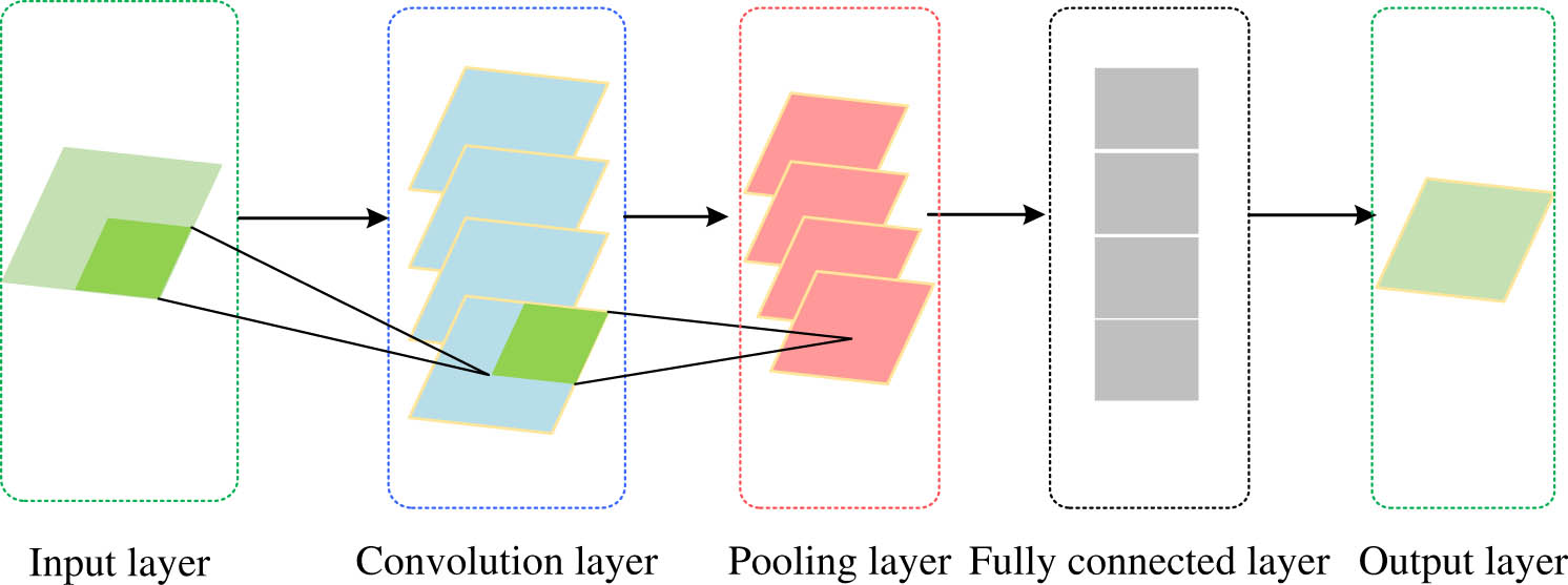
CNN basic structure diagram.

The advantage of CNN is that because convolutional layers share convolutional core parameters and have a smaller parameter size, it makes it easier to optimize the network structure. CNN needs deeper network layers to extract features more completely. However, the deeper the network, the easier it is for the gradient to disappear. Increasing the difficulty of training will lead to a decline in the performance of the model. For solving the CNN performance degradation, the application of residual unit to CNN models is studied. Then, we study the use of identity mapping and quick connections to reduce the gradient disappearance phenomenon in deep network training. The residual’s structure unit is shown in Figure 2, and the residual unit is implemented in the form of hop layer connections. It then adds the input of the unit directly to the output of the unit and is finally reactivated. 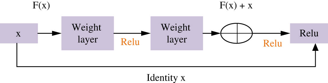In the figure, x is the input of the residual unit and F ( x ) is the residual. It is the output after the first layer of linear change and activation.

Figure 2

Schematic diagram of residual element structure.

If it is assumed that the output value of the upper layer of the residual unit is input to that layer, i.e., the input value of this layer is x m , then the output value x n can be expressed in the following equation [17]:

(1) x n = x m + F ( x m + w m ) ,

where w m is the weight. In a residual network, the input value X of this layer is added to F(x) before the activation of the second layer after a linear change. The study then performs post activation output, adding an X before activating the second layer output value. The name of this path is a shortcut connection. Equation (2) showcases this process [18]:

(2) F ( x m , w m ) = w m σ ( w n x n ) ,

where σ is the activation function. Through the recursive relationship, the expression of any deep unit x C is shown in the following equation [19]:

(3) x C = x m + ∑ m = 1 c − 1 F ( x m , w m ) .

The characteristics of an arbitrary deep element x C are equivalent to the characteristics of a shallow element l plus a residual function in the form of ∑ m = 1 c − 1 F ( x m , w m ) . It can be seen that there is a residual characteristic between any element and l. This feature ∑ m = 1 c − 1 F ( x m , w m ) can also be expressed in the following equation [20]:

(4) x C = ∑ m = 0 c − 1 F ( x m , w m ) + x 0 .

In equation (4), this feature can be considered as the sum of all residual function outputs plus the initial input x 0 . The ordinary CNN feature x _Cf is different from the residual function. The expression is given in the following equation [21]:

(5) x Cf = ∏ m = 0 c − 1 w m x 0 .

From the synthesis of equations (4) and (5), the residual network is essentially a summation operation; ordinary CNN performs quadrature operations, and the computational complexity of the residual network is far smaller than that of ordinary CNN. Deep neural networks are also prone to fitting problems during learning and training. This will reduce the training speed of the network. Therefore, this study introduces the batch normalization (BN) algorithm to alleviate these problems. The BN algorithm could normalize the input data of the network’s each layer, making its numerical mean value 0 and standard deviation 1. In addition, when performing data normalization processing, the BN algorithm can add two learnable parameters α and β to eliminate the impact without damaging the learned features of the upper layer network. Equation (6) indicates the following relationship:

(6) y ( k ) = α ( k ) x ˆ + β ( k ) ,

where y ( k ) represents the output of the k -th neuron. In a network, each neuron has a pair of α and β , and if they satisfy α ( k ) = Var [ x ( k ) ] and β ( k ) = E [ x ( k ) ] , respectively, they can learn to restore the distribution of features that need to be learned in addition to the original network. Var [ x ( k ) ] serves as the standard deviation of this batch of data; E [ x ( k ) ] represents the mean value. Equation (7) illustrates the forward propagation of the BN algorithm:

(7) μ b ← 1 m ∑ i = 1 m x i σ b ← 1 m ∑ i = 1 m ( x i − μ b ) 2 x ˆ l ← x i − μ b σ b 2 + E y m ← α x ˆ l + β = B N α , β ( x i ) ,

where y m and μ b 2 represent the numerical mean and variance; x i and y m represent the input data before normalization and output after normalization, respectively. The features from each layer of CNN are high-dimensional, with a large number of redundant feature information. To prevent the sharp increase in computational complexity caused by high dimensions from degrading the model’s generalization, a principal component analysis (PCA) dimensionality reduction algorithm was studied to reduce the feature dimensions. The addition of PCA technology can reduce the computational burden of deep feature fusion. This eliminates the interaction between the original data. The process of PCA converting sample x i into a new sample Z ( i ) is shown in the following equation:

(8) Z ( i ) = x i w t ,

where w t is the eigenvector matrix. After transformation, feature fusion is performed to obtain the new multi-level feature Features total of the following equation:

(9) Features total = PCA [ PCA ( p 8 ) ] FC 2 ,

where p 8 is the output result of the eighth pooling layer and FC serves as the output of the full connectivity layer. Based on the aforementioned optimization results, an improved CNN model is obtained. It is indicated in Figure 3. The model is composed of a convolutional layer, a fully connected layer, and a residual element. Each convolution layer uses a 3 × 3 convolution kernel for convolution operations and feature extraction. At this point, the study uses a normalization algorithm to speed up the network’s convergence. It uses the ReLU function to activate the extracted features. Then, the research output generates corresponding feature maps and introduces a pooling layer after the convolution layer for feature dimensionality reduction.

Figure 3

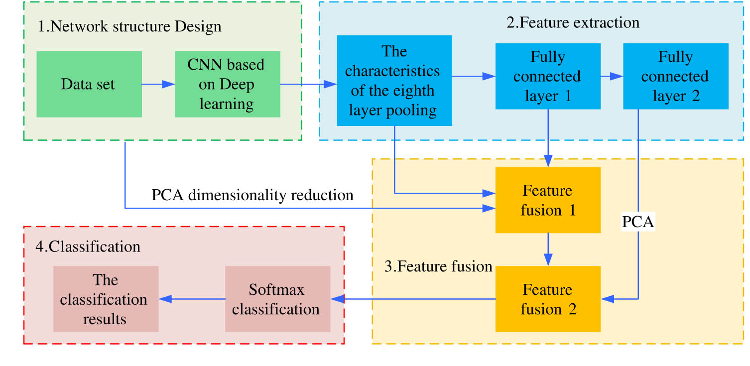
Improved CNN model structure.

3.2 Construction of PF prediction model based on LSTM and improved CNN

As an improved version of RNN, LSTM effectively reliefs the gradient disappearance phenomenon. It does well in sequence data with relatively long prediction intervals and delays. Therefore, the research combines it with improved CNN to construct a prediction model. Figure 4 illustrates the structure of the LSTM. It could preserve the long-term state of the unit, represented by horizontal lines running through the unit. The main part consists of three parts, namely, forgetting gate, input gate, and output gate. It combines short-term memory with long-term memory through gate control, which, to some extent, solves the gradient disappearance. In Figure 4, x t serves as the input on time t , y t serves as the output at that time, and σ is the sigmoid function. When information passes through the forgetting gate, it is determined which information needs to be forgotten. And it passes through an activation function to express whether the output is retained. Second, it is to calculate the information, which needs retaining, to participate in subsequent calculations. The next step is to fuse the screening results of the previous two steps to obtain a new value. And it forgets the part of the previous layer that has been used and lost value, and adds the value required for this layer, i.e., the information retained by the previous layer. After filtering, the information to be output is finalized through the sigmoid function, and finally output through the Tanh function [22].

Figure 4

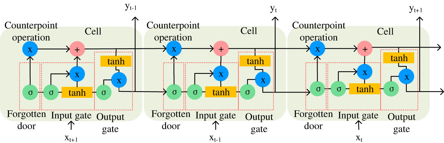
LSTM structure chart.

The forgetting gate of LSTM determines whether to discard the information through the sigmoid function. The equation for forgetting doors is shown in the following equation:

(10) F = sigmoid ( w F [ y t − 1 , x t ] ) ,

where w F serves as the weight of the forgetting gate, x t serve as the input at time t , and y t − 1 is the output at t − 1 time. The expressions for the update unit status of the input gate and the forgotten gate are shown in the following equation:

(11) C t = F × C t − 1 + tanh ( w z [ y t − 1 , x t ] ) × sigmoid ( w i [ y t − 1 , x t ] ) ,

where C t represents the new state, x z is the previous input value, I is the input gate at this time, and w i and w i represent the weights. The output gate equation is shown in the following equation:

(12) O = sigmoid ( w o [ y t − 1 , y t ] ) ,

where w o is the weight of the output gate. The output expression is shown in the following equation:

(13) y t = O × tanh ( C t ) .

The research spliced LSTM and improved CNN to obtain a PF prediction model. Figure 5 illustrates it. The model is composed of data input, data matrix, improved CNN layer, LSTM model layer, full connection layer, and output layer. The model will convert PF data into a data matrix and then select training set data to train the model. And the model uses improved CNN to extract features from PF data, time data, and weather data. Finally, it is converted into an input vector of the LSTM prediction model. Then, the study used LSTM models to train input vectors and compared them using validation sets. Then, it calculates the prediction results and errors and selects the model’s optimal parameters. Finally, the PF of the test set is predicted, and the prediction results using different models are evaluated, analyzed, and compared.

Figure 5

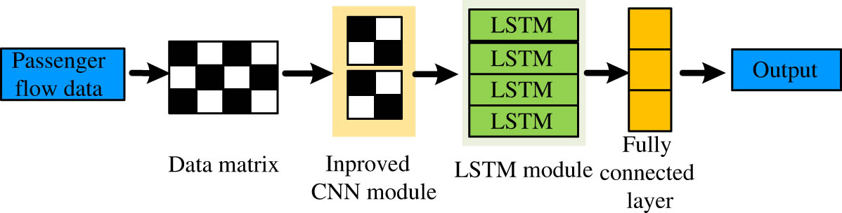
PF forecasting model.

No matter which method is used for PF prediction, there will inevitably be a certain degree of deviation. The magnitude of this deviation often determines the performance and accuracy of prediction methods. Therefore, this study will construct an indicator system to evaluate the PA and adaptability of the model based on prediction errors. The PA evaluation indicators of the model select several common error evaluation methods, namely, root mean square error (RMSE), normalized root mean square error (NRMSE), mean absolute percentage error (MAPE), and mean absolute error (MAE). The specific equation for each error evaluation method is shown in the following equation:

(14) RMSE = 1 n ∑ i = 1 n ( P ¯ i − P i ) 2 MAE = ∑ i = 1 n ∣ P i − P i ¯ ∣ n NRMSE = 1 n × ∑ i = 1 n ( P i − P i ¯ ) 2 P max − P min MAPE = ∑ i = 1 n P i − P i ¯ P i i n ,

where P ¯ is the predicted value, P i is the actual value, n serves as the quantity of samples, and P max and P min serve as the maximum and minimum values, respectively.

4 Analysis of the application results of the combined neural network-based PF forecasting model

The experiment selected a scenic spot in Hainan Province as the research object and selected the PF data of the whole year of 2020 for testing. Taking each hour as the statistical interval, the PF data of the entrance and exit of the scenic spot is sorted out, and the PF data of the entrance and exit is based on the PF data of working days and non-working days, respectively. In Keras, a deep learning framework based on Python language, a CNN + LSTM prediction model is constructed for the prediction study of PF.

In the experiment, the dataset was divided into a training set, a validation set, and a test set. The experiment normalized it before training. This experiment converts the processed PF data into a matrix using scientific computing libraries, such as Pandas and Numpy in Python, and segments the dataset. Second, the experiment uses Keras to establish a linear stacking model, stacking each layer in order. The model has two layers of CNN convolutional layer, the first layer contains 50 convolutional cores, and the second layer contains 20 convolutional cores. In addition, the convolution kernel size of the matrix used in the experiment is 3 × 3, the step size is 1, and the excitation function is Relu function. LSTM layers’ quantity is 1, neural cells’ quantity in the hidden layer is 50, and the learning rate is 0.001. Neurons’ quantity in the full junction layer is 50. The model uses the AAE as a loss function. The experiment uses a grid search method to test some of the model’s super parameters and select the optimal parameter results [23]. Due to the significant differences in the distribution of PF data between working and non-working days, grid search algorithms are utilized to find the optimal combination of hyperparameters for the model for both working and non-working days.

The AAE is used as an evaluation index in the experiment and is ranked in the descending order according to the validation set error. It is of great significance to discuss the variation trend of the AAE of the model during training. For this experiment, the AAE values of the CNN + LSTM model in the training set and the verification set after 50 training iterations on working and non-working days were counted. At the same time, the experiment used the MAE index to measure the training process of the improved CNN + LSTM model. Then, it is necessary to test the effectiveness of the BN algorithm. Therefore, the distribution of activation function output values for networks with and without BN is compared. To observe the variation of the predicted deviation of the model over time, this experiment plotted a numerical curve between the predicted value of the model and the actual value of the total PF within 200 h. To observe the performance of this research model in a horizontal comparison, the experiment compares it with the adaptive multiscale ensemble (AME) learning method in the literature [24] and the integrated empirical mode decomposition, deep belief network, and ensemble empirical mode decomposition - deep belief network (EEMD-DBN) model of Google Trends in literature [24]. MAE, NRMSE, and RMSE were used as evaluation indicators for comparing the results. Finally, the number of inbound and outbound tourists predicted by this research model is counted throughout the year.

Table 1 demonstrates the grid search results for both weekday and non-weekday models. Table 1 shows that on weekdays, when batches’ quantity, neurons’ quantity in the LSTM layer, and iterations’ quantity are 10, 50, and 50, respectively, the performance of the deep learning model reaches its optimal level. Therefore, the study will build a CNN + LSTM model based on the optimal combination of hyperparameter values to predict weekday PF data. On non-working days, when batches’ quantity, neurons’ quantity in the LSTM layer, and iterations’ quantity are 10, 100, and 50, respectively, and the model achieves optimal performance. Therefore, the study will build a CNN + LSTM model based on the optimal combination of hyperparameter values to predict non-working day PF data.

Table 1

Partial results of the grid search in the weekday and non-workday models

	Batch size	Number of LSTM layer neurons	Iteration number	Training set error	Validation set error
Working day	10	50	50	44.44	39.80
	5	100	20	51.00	44.10
	10	50	50	49.50	45.70
	10	50	100	40.64	55.89
	10	100	50	44.33	27.29
Non-working days	5	200	20	86.50	31.33
	10	100	20	68.21	28.95
	5	50	100	45.01	31.41
	10	150	20	57.93	32.06

Figure 6 showcases the MAE values of the improved CNN + LSTM model in the training set and validation set. Figure 6(a) indicates the MAE’s change rule with the increase of training times on two sets of the model on the workday. The statistical results in Figure 6(a) illustrate that the AAE of the model decreases quickly initially and stabilizes as the number of training iterations increases gradually. When training iterations’ quantity reaches 50, the model keeps stable. However, if the model continues to increase training iterations’ quantity at this time, it may lead to the model’s overfitting. It influences the test set’s accuracy. According to the statistical results in Figure 6(b), the AAE of the model first decreases rapidly and then gradually stabilizes as the number of training iterations increases. After 50 training iterations, the CNN + LSTM model keeps stable.

Figure 6

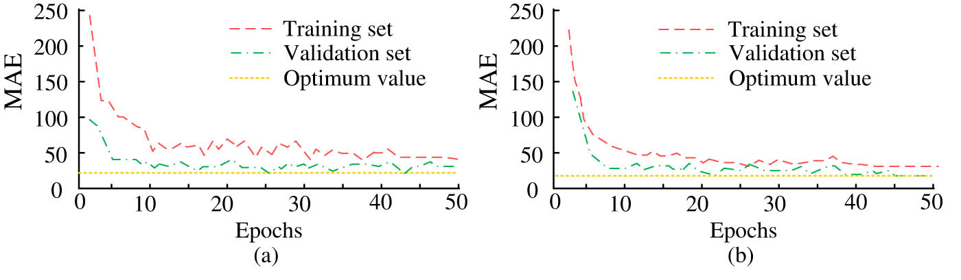
Error curves for business days and non-business days. (a) Working day MAE error curve. (b) Non-working day MAE error curve.

For networks with and without BN algorithms, Figure 7 showcases the input and output distributions of their activation functions. The figure indicates that the input of the activation function of the network with BN is concentrated in the sensitive region. And accordingly, its corresponding derivative is relatively large. This will be conducive to in-depth learning of the network. The input distribution without BN network is relatively scattered. After BN, the output of the network is relatively smooth, with many values at both the saturation stage and the activation stage. This will help the network to more effectively utilize tanh for non-linear transformation during learning. The network output without BN is only distributed at both ends, indicating that its output is at a saturation stage, with most values of 1 or −1. This is not conducive to online learning. It can be seen that the addition of BN effectively improves the learning performance of the network.

Figure 7

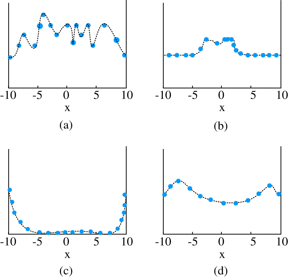
Input and output distribution of activation function with and without BN. (a) No BN activation function input distribution. (b) Input distribution of activation function added to BN. (c) No BN activation function output distribution. (d) Joined the BN activation function of the output distribution.

Within 200 h, the comparison between the two values of the model’s total PF on working and non-working days is shown in Figure 8. The predicted PF and real PF curves in Figure 8(a) indicate that although the real PF curve has strong volatility, the model in this study can still accurately predict. These two values can well complete the fitting. The predicted PF and real PF curves in Figure 8(b) indicate that the research model can still accurately predict the PF during non-working days. The longer the time, the higher the accuracy of the prediction. This shows that this research model can also learn the changing rules of PF data and obtain better prediction results.

Figure 8

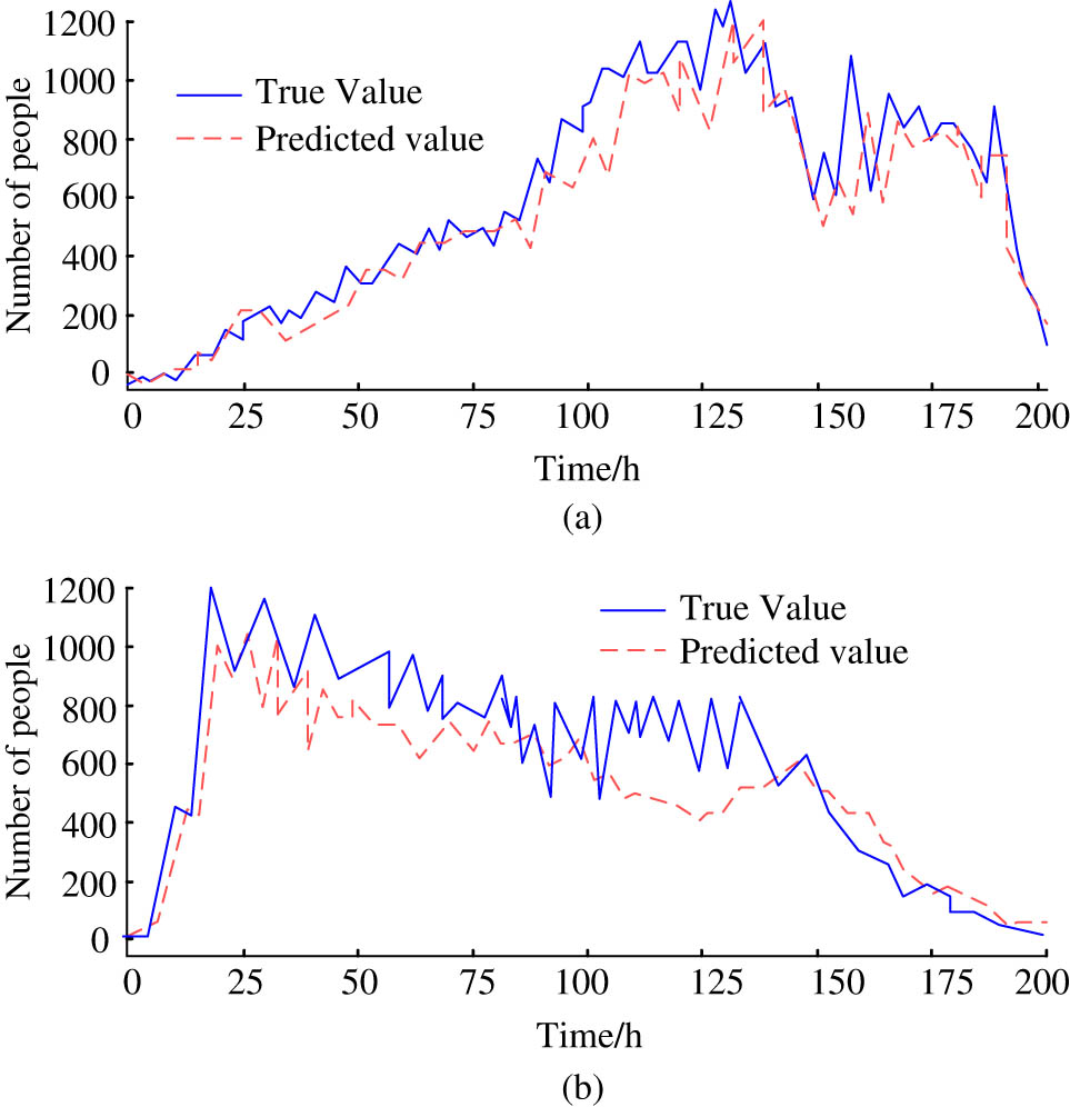
Forecast results for business and non-business days. (a) Workday forecast results. (b) Non-workday forecast results.

Table 2 indicates the comparison of various models. The table indicates that the inflow RMSE of this research model is 82.51 and the outflow RMSE is 89.80. The inflow and outflow MAEs are 26.92 and 30.91; the inflow and outflow NRMSEs are 3.99 and 3.94; the inflow and outflow MAPEs are 1.55 and 1.53. The model error in this study is smaller than other models.

Table 2

Comparison results of each model

Index	This study model	AME model	EEMD-DBN model
RMSE(Inflow)	82.51	109.02	98.00
RMSE(Outflow)	89.80	117.39	107.90
MAE(Inflow)	26.92	45.11	43.00
MAE(Outflow)	30.91	49.55	45.74
NRMSE(Inflow)	3.99	5.20	11.00
NRMSE(Outflow)	3.94	5.13	11.21
MAPE(Inflow)	1.55	2.10	4.33
MAPE(Outflow)	1.53	2.07	4.28

Figure 9 indicates that on the same day, the comparison results of the inflow forecast values of each model. It demonstrates that this research model’s predicted value fits the true value best. This is also a relatively accurate study of the law of change in real values. Although the EEMD-DBN model is also relatively close to the true value during the 06:00 to 16:00 time period. According to Figure 9, the inflow of tourists to the scenic spot is concentrated in the early morning and gradually decreases in the future.

Figure 9

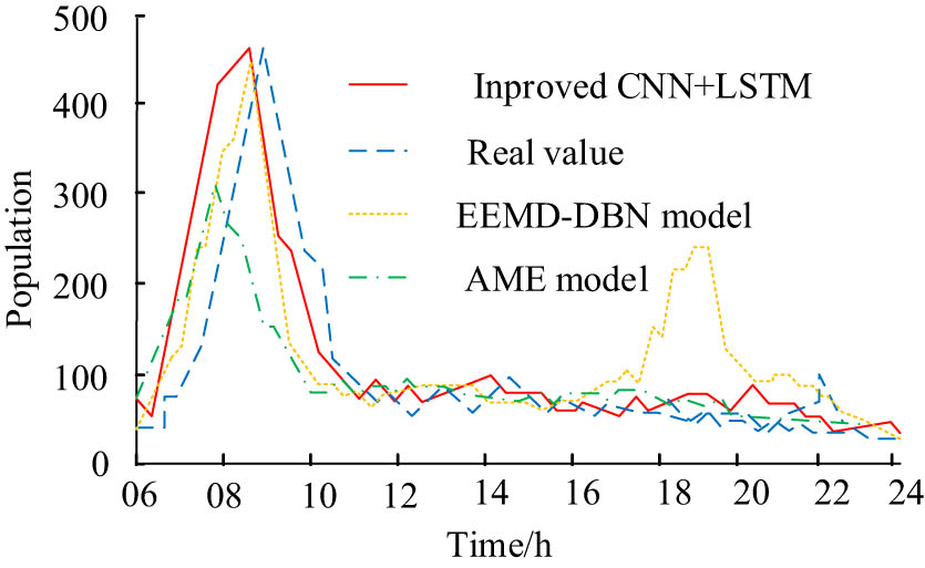
Comparison results of inflow predictions.

Throughout the year, the characteristics of tourist inflow and outflow predicted by the model in this scenic area are shown in Figure 10. It can be seen from the figure that the tourist volume of this scenic spot has obvious temporal characteristics. Taking every four months as a cycle, there are high inflow peaks in winter, spring, and summer. January and December were the most traffic, with inflows up to 5,000. The inflow in July is a small peak, and the highest inflow can be about 3,000 people large. The possible reason is that the city has a warm climate in winter and spring, with a large influx of tourists; due to the existence of longer holidays in July, August, and October, the inflow increased accordingly. The outflow trend is roughly the same, maintaining a high inflow while maintaining a high outflow. In the off-season, the PF of the scenic spot remains below 1,000 people. Through the aforementioned analysis of the PF of the scenic spot, we can see that the off-season and peak season differ greatly.

Figure 10

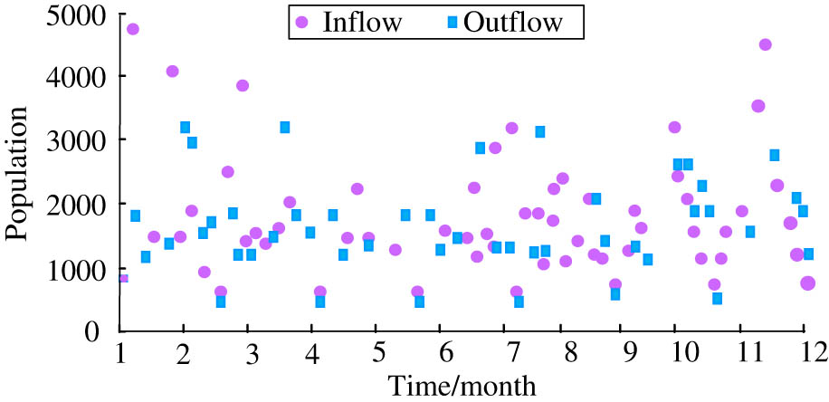
PF time distribution characteristics.

In order to increase the off-season PF of the scenic spot, the following aspects can be considered: first of all, off-season discount or package discount to attract tourists to patronize the scenic spot in the off-season. Second, cooperate with local residents or enterprises to launch the special products of off-season tourism. For example, we will organize farmhouse music experience and folk culture activities to attract more tourists. Finally, we can increase the publicity of off-season tourism through the Internet, social media, and tourism media. Show the unique charm and special discounts of the scenic spot in the off-season to attract the attention of tourists.

5 Conclusion

In the season when tourists come in droves, accurately predicting the number of tourists is the top priority of scenic area operation. Therefore, this study established a prediction model based on an improved CNN and LSTM combined neural network to forecast the inflow and outflow of tourists in scenic spots. The experimental results show that on weekdays, when batch processes’ quantity, LSTM layer neurons’ quantity, and iterations’ quantity are 10, 50, and 50, respectively, and on non-weekdays, when batch processes’ quantity, LSTM layer neurons’ quantity, and iterations’ quantity are 10, 100, and 50, respectively, the model performance reaches the optimal level. The inflow RMSE of this research model is 82.51; the outflow RMSE is 89.80; the inflow and outflow MAEs are 26.92 and 30.91; the inflow and outflow NRMSEs are 3.99 and 3.94; the inflow and outflow MAPEs are 1.55 and 1.53. The model error in this study is smaller than other models. Winter, summer, and autumn are the peak tourist seasons in the study area. At this time, the scenic spot needs to increase management and operation investment and implement a certain degree of flow restriction to meet the tourist demand. However, there are many superparameters, and the desirable space for setting is discrete values. The disadvantage of this study is that the influence of special events such as large-scale events and sudden large PF is not studied. In the future, the relationship with large-scale events and sudden large PF should be studied after collecting sufficient data in the future.

Funding information: The author states no funding involved.
Author contributions: All work for this article was done by Fang Yin.
Conflict of interest: The author have no relevant financial or non-financial interests to disclose.
Data availability statement: All data generated or analyzed during this study are included in this article.

References

[1] Du S, Bahaddad AA, Jin M, Zhang Q. Research on the tourist flow feature of scenic area based on fractal statistical model – A case of zhangjiajie. Fractals. 2022;30(2):2240103.1–2.10.1142/S0218348X2240103XSuche in Google Scholar

[2] Ding X, Liu Z, Xu H. The passenger flow status identification based on image and WiFi detection for urban rail transit stations. J Vis Commun Image Represent. 2019;58(JAN):119–29.10.1016/j.jvcir.2018.11.033Suche in Google Scholar

[3] Sajanraj TD, Mulerikkal J, Raghavendra S, Vinith R, Fábera V. Passenger flow prediction from AFC data using station memorizing LSTM for metro rail systems. Czech Tech Univ Prague – Cent Library. 2021;31(3):173–89.10.14311/NNW.2021.31.009Suche in Google Scholar

[4] He Y, Zhao Y, Tsui KL. Modeling and analyzing modeling and analyzing impact factors of metro station ridership: An approach based on a general estimating equation factors influencing metro station ridership: An approach based on general estimating equation. IEEE Intell Transp Syst Mag. 2020;12(4):195–207.10.1109/MITS.2020.3014438Suche in Google Scholar

[5] Muniz E, Dandolini GA, Biz AA, Ribeiro AC. Customer knowledge management and smart tourism destinations: a framework for the smart management of the tourist experience–SMARTUR. J Knowl Manag. 2021;25(5):1336–61.10.1108/JKM-07-2020-0529Suche in Google Scholar

[6] Huang W, Cao B, Li X, Zhou M. Stations based on spatio-temporal graph convolutional network with periodic components. J Circuits Syst Comput. 2022;31(7):2250134.1–18.10.1142/S0218126622501341Suche in Google Scholar

[7] Jing Z, Yin X. Neural network-based prediction model for passenger flow in a large passenger station: An exploratory study. IEEE Access. 2020;8:36876–84.10.1109/ACCESS.2020.2972130Suche in Google Scholar

[8] Zhang Z, Wang C, Gao Y, Chen Y, Chen J. Passenger flow forecast of rail station based on multi-source data and long short term memory network. IEEE Access. 2020;8:28475–83.10.1109/ACCESS.2020.2971771Suche in Google Scholar

[9] Nagaraj N, Gururaj HL, Swathi BH, Hu YC. Passenger flow prediction in bus transportation system using deep learning. Multimed Tools Appl. 2022;81(9):12519–42.10.1007/s11042-022-12306-3Suche in Google Scholar PubMed PubMed Central

[10] Lu T, Yao E, Liu S, Zhou W. Short-time forecast of entrance and exit passenger flow for new line of urban rail transit during growth period. Tiedao Xuebao/J China Railw Soc. 2020;42(5):19–28.Suche in Google Scholar

[11] Zhang H, He J, Bao J, Hong Q, Shi X. A hybrid spatiotemporal deep learning model for short-term metro passenger flow prediction. J Adv Transp. 2020;2020(Pt.4):4656435.1–12.10.1155/2020/4656435Suche in Google Scholar

[12] He Y, Li L, Zhu X, Tsui KL. Multi-graph convolutional-recurrent neural network (MGC-RNN) for short-term forecasting of transit passenger flow. IEEE Trans Intell Transp Syst. 2022;23(10):18155–74.10.1109/TITS.2022.3150600Suche in Google Scholar

[13] Qian ZA, Xi B, Ss C, Dy A. A two-layer modelling framework for predicting passenger flow on trains: A case study of London underground trains. Transp Res Part A: Policy Pract. 2021;151:119–39.10.1016/j.tra.2021.07.001Suche in Google Scholar

[14] Zhang S, Wu Y, Men C, Ren N, Li X. Channel compression optimization oriented bus passenger object detection. Math Probl Eng. 2020;2020(Pt.6):3278235.1–11.10.1155/2020/3278235Suche in Google Scholar

[15] Fu X, Zuo Y, Wu J, Yuan V, Wang S. Short-term prediction of metro passenger flow with multi-source data: A neural network model fusing spatial and temporal features. Tunn Undergr Space Technol. 2022;124(Jun):104486.1–14.10.1016/j.tust.2022.104486Suche in Google Scholar

[16] Goumas SK, Kontakos S, Mathheaki AG, Xristoforidis S. Modeling and forecasting of tourist arrivals in crete using statistical models and models of computational intelligence: A comparative study. Int J Oper Res Inf Syst. 2021;12(1):58–72.10.4018/IJORIS.2021010105Suche in Google Scholar

[17] Shehab LH, Fahmy OM, Gasser SM, El-Mahallawy MS. An efficient brain tumor image segmentation based on deep residual networks (ResNets). J King Saud Univ-Eng Sci. 2021;33(6):404–12.10.1016/j.jksues.2020.06.001Suche in Google Scholar

[18] Wang H, Miao F. Building extraction from remote sensing images using deep residual U-Net. Eur J Remote Sens. 2022;55(1):71–85.10.1080/22797254.2021.2018944Suche in Google Scholar

[19] Shu Z, Liu Z, Zhou J, Tang SZ, Yu ZT, Wu SJ. Spatial–spectral split attention residual network for hyperspectral image classification. IEEE J Sel Top Appl Earth Obs Remote Sens. 2022;16:419–30.10.1109/JSTARS.2022.3225928Suche in Google Scholar

[20] Yu H, Cheng X, Chen C, Heidari AA, Liu JW, Cai ZN, et al. Apple leaf disease recognition method with improved residual network. Multimed Tools Appl. 2022;81(6):7759–82.10.1007/s11042-022-11915-2Suche in Google Scholar

[21] Zhang RF, Li MC. Bilinear residual network method for solving the exactly explicit solutions of nonlinear evolution equations. Nonlinear Dyn. 2022;108(1):521–31.10.1007/s11071-022-07207-xSuche in Google Scholar

[22] Bi D, Xing G, Sun S, Guo J, Wang S. Seasonal and trend forecasting of tourist arrivals: An adaptive multiscale ensemble learning approach. Int J Tour Res. 2022;24(3):425–42.10.1002/jtr.2512Suche in Google Scholar

[23] Priyadarshini I, Cotton C. A novel LSTM–CNN–grid search-based deep neural network for sentiment analysis. J Supercomput. 2021;77(12):13911–32.10.1007/s11227-021-03838-wSuche in Google Scholar PubMed PubMed Central

[24] Xiao Y, Tian X, Liu JJ, Cao G, Dong Q. Tourism traffic demand prediction using google trends based on EEMD-DBN. Engineering. 2020;12(3):194–215.10.4236/eng.2020.123016Suche in Google Scholar

Received: 2023-09-11

Accepted: 2024-01-09

Published Online: 2024-03-26

This work is licensed under the Creative Commons Attribution 4.0 International License.

Artikel in diesem Heft

https://doi.org/10.1515/jisys-2023-0158

Schlagwörter für diesen Artikel

CNN; BN; residual unit; LSTM; passenger flow forecast

Creative Commons

BY 4.0