Application of a mixed additive and multiplicative random error model to generate DTM products from LiDAR data

Guohong Li; Huijuan Xin; Xiaohui Song; Khan Rehan

doi:10.1515/geo-2025-0809

Article Open Access

Application of a mixed additive and multiplicative random error model to generate DTM products from LiDAR data

Guohong Li , Huijuan Xin , Xiaohui Song and Khan Rehan

Published/Copyright: May 28, 2025

Published by

Become an author with De Gruyter Brill

Submit Manuscript Author Information

From the journal Open Geosciences Volume 17 Issue 1

Abstract

Digital terrain model (DTM) has wide-ranging applications in numerous fields, including natural resource management, urban planning, environmental protection, and disaster monitoring. Utilizing LiDAR data to generate DTM is now a mainstream method. In current applications, LiDAR data are still treated as having primarily additive errors; however, studies have shown that it is affected by both additive and multiplicative errors. From the perspective of error theory and surveying adjustment, it is theoretically inappropriate to treat mixed additive and multiplicative errors directly as additive errors, as each error model is based on a distinct theoretical framework. In view of this, we applied the mixed additive and multiplicative error theory to the generation of LiDAR-derived DTM products and validated its accuracy through two real measurement cases and one simulation case. The experimental results demonstrate that the mixed additive and multiplicative errors theory provides higher accuracy than the additive error theory in both DTM fitting and interpolation. This confirms that incorporating the mixed additive and multiplicative error theory into DTM product generation is beneficial.

Keywords: digital terrain model; mixed additive and multiplicative random errors model; additive errors; LiDAR

1 Introduction

Digital terrain model (DTM) enables the digital simulation of ground topography using limited elevation data, offering broad applications across fields such as natural resources management, urban planning, environmental protection, and disaster monitoring. For example, in natural resource management, DTM supports terrain analysis, geological surveys, and water resource management; in urban planning, it assists with three-dimensional modeling of cities, transportation planning, and landscape design; in disaster monitoring, it aids in flood simulation and seismic disaster assessment [1,2,3]. Currently, generating DTM from LiDAR data is a mainstream method [4]. The original LiDAR data comprise ground points and feature points. To generate a DTM, the point cloud data must be filtered, specifically by eliminating the feature points; thus, the primary research focus in generating a DTM involves removing the non-ground points from the point cloud data. Research in this area is documented in previous studies [5,6,7,8,9,10,11,12]. After obtaining the ground points, DTMs are generated using methods such as primary trend surface fitting, secondary trend surface fitting, cubic spline interpolation, and Bezier surfaces [11,13].

The quality of LiDAR data significantly influences the accuracy of the DTM, making it essential to evaluate LiDAR data accuracy. Gillin et al. [14] analyzed the accuracy of radar datasets obtained by the Optech GEMINI Airborne Laser Terrain Mapper using ground checkpoint data, and a difference ranging from 0.7 to 2.10 m was observed between the datasets. Contreras et al. [15] evaluated the accuracy of two LiDAR point cloud datasets collected during the leaf-off season, and the results indicated that the root mean square error (RMSE) of the elevation difference between LiDAR and GPS coordinates was 0.75 m. Sibona et al. [16] comparatively analyzed radar data collected by the Optech™ ALTM 3100 EA LiDAR sensor in a forested area using GPS data, reporting an average elevation difference of approximately 0.10 m and an RMSE of 1.25 m when compared with GPS data. Guerra-Hernández et al. [17] compared the accuracy and effectiveness of point clouds obtained by airborne laser scanners (ALSs) and unmanned aircraft systems (UASs) in detecting and measuring individual tree heights. Kovanič et al. [18] compared the accuracy of point cloud data acquired by the Riegl LMS-Q780 scanner with that from the DJI Phantom 4 Pro UAS. Cățeanu and Ciubotaru [19] evaluated the accuracy of nine commonly used interpolation methods using Riegl LMS-Q560 data with cross-validation. These studies demonstrate the feasibility and effectiveness of using LiDAR data for DTM generation. Scholars have also developed various methods to assess the accuracy of measurement systems and analyze the sources of errors. For instance, Eren and Hoşbaş [20] analyzed measurement precision using a specialized experimental setup designed to monitor structural movements via video cameras or from an error modeling perspective to enhance the accuracy of trend estimation. For example, Erkoç and Doğan [21], in their analysis of altimeter and tide gauge data, found that error modeling played a crucial role in different datasets. Alternatively, machine learning techniques have been incorporated into geographical analysis [22]. All of these studies aim to ensure the accuracy of the data used or to extract more meaningful information from it.

To date, in the aforementioned studies, the algorithms for interpolating to obtain DTMs are based on the additive error model, also known as the Gauss–Markov model. The model is expressed as follows:

(1) y i = f i ( β ) + ε i , i = 1 , 2 , … . n

or equivalently in matrix form

(2) y = f ( β ) + ε .

Stochastic model:

(3) E ( ε ) = 0 D ( ε ) = W σ 2 = P − 1 σ 2 .

Here, f i ( β ) are linear (or nonlinear) functions of β , β is a t-dimensional unknown real-valued vector to be estimated, E ( ⋅ ) is the expectation symbol, D ( ⋅ ) is the variance symbol, ε i are the random errors of y i , P denotes the weights of the observations, W represents the covariance factor matrix, also known as the weight inverse matrix, where W = P − 1 , σ 2 is a positive unknown scalar, also referred to as the unit weight variance, and y i are measurements.

However, it has been shown that LiDAR data are subject to a mixture of multiplicative and additive errors [1,2,3]. In other words, the accuracy of LiDAR measurements may decrease as the distance increases. However, when field measurements of LiDAR were collected and used to generate DTMs, it was shown in previous studies [23,24] that the accuracy of LiDAR measurements may also depend on the slopes of a terrain. At this juncture, it is clearly inappropriate to apply the additive error theory to this issue [25]. In fact, within geodesy, various datasets are affected by both multiplicative and additive errors, including electronic distance measurement (EDM), global positioning system (GPS), and very long baseline interferometry (VLBI) [26,27]. For these observations, accuracy is typically expressed using the following equation:

(4) ε L = ε a + L ∗ ε b .

Here, ε L denotes the random error of the observation L, and ε a and ε b are usually referred to as the fixed and proportional errors (multiplicative errors), which are independent of each other. Xu et al. [28] proposed a mixed additive multiplicative error model to deal with such observations as follows:

(5) y = f 1 ( β ) 0 ⋱ 0 f n ( β ) ( 1 + ε b ) + ε a .

With the notation of the Hadamard’s product of matrices/vectors, model (5) can be rewritten as follows:

(6) y = f ( β ) ⊙ ( 1 + ε b ) + ε a .

Here, f ( β ) are linear (or nonlinear) functions of β , β is a t-dimensional unknown real-valued vector to be estimated, ε b represents the multiplicative error that follows a normal distribution, ε a represents the additive error that also follows a normal distribution, and ⊙ stands for the Hadamard’s product of matrices/vectors. The rule of thumb is that matrices or vectors of the same dimension are multiplied by the corresponding positional elements. For example,

A = a 11 a 12 a 13 a 21 a 22 a 23 a 31 a 32 a 33 B = b 11 b 12 b 13 b 21 b 22 b 23 b 31 b 32 b 33 , A ⊙ B = a 11 b 11 a 12 b 12 a 13 b 13 a 21 b 21 a 22 b 22 a 23 b 23 a 31 b 31 a 32 b 32 a 33 b 33 .

Comparing equations (2) and (6), the function model reveals that the mixed additive and multiplicative error model more accurately represents the observation’s accuracy information than the additive error model does.

Based on the foregoing analysis, this study focuses on the accuracy of the mixed additive and multiplicative error model in DTM applications. The structure of this article is organized as follows: Section 2 introduces the principles of the mixed additive and multiplicative error model; Section 3 verifies the model’s accuracy using a DTM case study; and Section 4 briefly summarizes the content of this article.

2 Mixed additive and multiplicative random error model

Equation (6) lists the mixed additive and multiplicative error model expressions. In this study, we only explore the case where f ( β ) is linear, at which point equation (6) can be rewritten as follows:

(7) y = ( X β ) ⊙ ( 1 + ε b ) + ε a .

Here, X represents a known coefficient matrix, with other symbols maintaining the same meanings as in equation (6). The most crucial issue at this point is how to utilize the observation data y , the coefficient matrix X , as well as the multiplicative error ε b and the additive error ε a , to solve for the unknown parameter β .

Assume that ε b follows a normal distribution with expectation 0 and variance ∑ b , and that ε a follows a normal distribution with expectation 0 and variance ∑ a . ε b are independent of each other, ε a are independent of each other, and ε a and ε b are independent of each other. For equation (7), find the expectation and variance of the observations:

(8) E ( y ) = X β ,

(9) ∑ y = D X β ∑ b D X β + ∑ a .

Here D X β = diag ( x i β ) denotes the diagonal matrix whose ith diagonal element is x i β . The principle of least squares is applied to equation (7) to find the least-squares solution:

(10) β ˆ LS = ( X T X ) − 1 X T y .

The least-squares solution is unbiased. The weighted least-squares (WLS) criterion is applied to equation (7):

(11) min : F ( β ) = ( y − X β ) T ∑ y − 1 ( y − X β ) .

Following the definition of derivatives of a scalar function with respect to a vector (or a matrix) [29], the partial derivative of the function F ( β ) is taken and made zero:

(12) 2 X T ∑ ˆ y − 1 ( y − X β ˆ ) + G ( y − X β ˆ ) T = 0 .

Here, G = [ ( y − X β ˆ ) T P ˆ 1 , ( y − X β ˆ ) T P ˆ 2 , … , ( y − X β ˆ ) T P ˆ t ] T , P ˆ i = ∂ ∑ y − 1 / ∂ β i .

According to Theorem 3 in the study of Magnus and Neudecker [29], the matrix P ˆ i can be written in the following form:

(13) P ˆ i = − ∑ ˆ y − 1 D X e i ∑ b D ˆ X β + D ˆ X β ∑ b D X e i ∑ ˆ y − 1 ,

where D X e i is a diagonal matrix with its kth diagonal element being equal to ( x k e i ) , e i is the ith natural basis vector of dimension t, and D ˆ X β is the estimate of D X β by replacing β with its corresponding WLS estimate β ˆ .

Substituting equation (13) into equation (12) yields

(14) X T ∑ ˆ y − 1 ( y − X β ˆ ) + G 1 ( y − X β ˆ ) = 0 .

Here,

G 1 = ( y − X β ˆ ) T ∑ ˆ y − 1 D X e 1 ∑ b D ˆ X β ∑ ˆ y − 1 ( y − X β ˆ ) T ∑ ˆ y − 1 D X e 2 ∑ b D ˆ X β ∑ ˆ y − 1 ⋮ ( y − X β ˆ ) T ∑ ˆ y − 1 D X e 3 ∑ b D ˆ X β ∑ ˆ y − 1

From equation (14), it is evident that the weighted least-squares solution is not analytical and must be obtained numerically through iterative methods; this solution is classified as a biased estimate [28]. The following equation is commonly used for the iterative solution:

(15) β ˆ k + 1 = X T ∑ ˆ y k − 1 X − 1 X T ∑ ˆ y k − 1 y − G 1 k ( y − X β ˆ ) . k = 0 , 1 , … .

The results of Xu et al. [28] indicate that the bias in the weighted least-squares estimates arises solely from the dependence of ∑ y on β . More precisely, this bias is attributed entirely to the second term on the left-hand side of equation (14). Following the approach suggested by Xu and Shimada [25], the second term can be removed from equation (14) to eliminate the bias in the weighted least-squares estimates. Equation (14) is thus rewritten as follows:

(16) X T ∑ ˆ y − 1 ( y − X β ˆ bc ) = 0 .

solving

(17) β ˆ bc = X T ∑ ˆ y − 1 X − 1 X T ∑ ˆ y − 1 y .

β ˆ bc is called the bias-corrected weighted least-squares solution. Again, the numerical solution can only be obtained by iterative methods. The following iterative methods are commonly used:

(18) β ˆ bc k + 1 = X T ∑ ˆ y k − 1 X − 1 X T ∑ ˆ y k − 1 y , k = 0 , 1 , … ,

where ∑ ˆ y k − 1 stands for ∑ ˆ y − 1 but is computed at point β ˆ bc k . Alternatively, a Gaussian Newton method can be used for the calculation:

(19) β ˆ bc k + 1 = β ˆ bc k − ( X T ∑ ˆ y k − 1 X ) − 1 X T ∑ ˆ y k − 1 ( y − X β ˆ bc k ) . k = 0 , 1 , … .

For computational theory, see refs [30,31,32]. For a detailed description of the mixed additive and multiplicative error model, the reader is referred to refs [25,28].

The algorithm for calculating β ˆ bc in the article is as follows.

Bias-corrected weighted least-squares algorithms
1. Initial value: Substitute the observation y and coefficient matrix X into equation (10) to obtain the least-squares solution β ˆ LS as the initial solution.
2. Iteration: Use the initial value to perform the following iterative operations:
D X β i = diag ( X β i )
∑ y i = D X β i ∑ b D X β i + ∑ a
β ˆ bc i + 1 = X T ∑ ˆ y i − 1 X − 1 X T ∑ ˆ y i − 1 y
Stop condition: when ∥ β ˆ bc i + 1 − β ˆ bc i ∥ ≤ 10 − 6 holds; otherwise g,o to i + 1 iterations.
3. Output: convergence after i iterations, and the solution is β ˆ bc .

3 Cases and analysis

3.1 Case 1

We employ LiDAR data in generating a DTM as a case study to validate the accuracy of the mixed additive and multiplicative error model. Given that LiDAR data are known to exhibit both multiplicative and additive errors, it is implied that the ground points obtained through filtering retain these errors.

The OpenGF dataset is an exceptionally large-scale ground filtering dataset derived from globally available ALS point clouds. The primary objective is to provide high-quality training and testing samples for ground filtering algorithm research, utilizing precisely labeled ground and non-ground point cloud data. The dataset spans an area of over 47 km² and encompasses nine distinct terrain scenarios from four different countries. Through the integration of globally available ALS point cloud data, OpenGF can rapidly generate large-scale datasets while maintaining data diversity and high quality.

Case 1 utilizes the OpenGF dataset for this study due to the following reasons:

Data scale and diversity: The OpenGF dataset comprises over 542 million accurately labeled point clouds, covering a broad range of terrain scenarios, including urban, mountainous, and vegetation-covered areas, thereby meeting diverse research needs.
High-quality labeling: The point cloud data in the dataset are meticulously labeled to ensure the accuracy of both ground and non-ground points.
Openness and extensibility: The OpenGF dataset is built on open data, making it easily accessible and extendable, and it supports global-scale research and applications. The dataset is available for download at (https://github.com/Nathan-UW/OpenGF).

A mountainous area from the dataset was selected as the case study for this study. The data from this mountainous area are presented in Figure 1.

Figure 1

Mountainous area data (Case 1).

The OpenGF dataset allows for the extraction of ground point data, excluding non-ground points. Figure 1 displays the ground point data from this mountainous area, with non-ground points, such as vegetation, removed. This mountainous region features both gentle and sloping areas, characterized by pronounced changes in relief, making it a complex terrain area. The x-coordinates range from 276,600 to 276,770 m, while the y-coordinates range from 4,868,500 to 4,868,700 m, with a total of 11,578 data points and an average density of 0.34 points per square meter (following the removal of a significant number of non-ground points).

Currently, no academic studies comprehensively analyze the multiplicative and additive errors in ground points obtained from LiDAR data, and analyzing these errors in actual observation data is complex. Therefore, this study will not address the separation of additive and multiplicative errors in the observed data at this stage but will assume the observed data as accurate and proceed by modeling the errors.

In the literature [33,34,35,36,37], the following equation is used for DTM fitting:

(20) h ( x , y ) = β 1 + β 2 x + β 3 y + β 4 x y + β 5 x 2 + β 6 y 2 .

The case study in this study also employs the aforementioned formula. The case specifies the standard deviation of the multiplicative error at 0.002 and the additive error at 0.15 m. Data influenced by the multiplicative and additive errors are depicted in Figure 2.

Figure 2

Experimental data affected by errors.

From the analysis above, treating LiDAR noise as an additive error aligns with the least-squares solution described in this study, as the formulas are consistent. Considering that both multiplicative and additive errors are involved, this approach corresponds to the bias-corrected weighted least-squares solution. To compare the accuracy of the two algorithms, three indices – MSE, MAE, and R ² (coefficient of determination) – are selected as the evaluation criteria. The formulas for these metrics are as follows:

(21) MSE = 1 n ∑ i = 1 n ( y ˆ i − y i ) 2 ,

(22) MAE = 1 n ∑ i = 1 n ∣ y ˆ i − y i ∣ ,

(23) R 2 = 1 − ∑ i = 1 n ( y ˆ i − y i ) 2 ∑ i = 1 n ( y i − y ¯ ) 2 ,

where y ˆ i denotes the predicted value, y i denotes the observed value, and y ¯ denotes the mean of the observations. The experiments were carried out as planned, and the fitting errors of the least squares (LS) and bias-corrected weighted least-squares methods (BC) were obtained, as shown in Figure 3.

Figure 3

LS method (left) and BC method (right) fitting errors.

Figure 3 (left) illustrates the error generated by applying the additive error model to fit the ground points, with errors ranging within ±10 m, the majority of which are concentrated within ±5 m. Figure 3 (right) illustrates the error generated by applying the mixed additive and multiplicative error model to fit the ground points, with errors also within ±10 m, most of which are concentrated in the ±5 m range. A comparison of Figure 3 (left and right) reveals that it is difficult to intuitively determine which model is more accurate based solely on the graphs. Since the fitting errors of both algorithms fall within the ±10 m range, this may raise doubts regarding the effectiveness of the algorithms. It is important to note that this study focuses solely on the accuracy of the two algorithms and not the accuracy of the DTM derived from the fitting, as DTM accuracy is influenced by the choice of the fitted model, ground undulation, and the extent of the ground range. As shown in Figure 1, the case area features complex terrain that may be difficult to describe using a standard mathematical formula. Therefore, this study focuses solely on the accuracy of the two algorithms in the context of the selected fitting model.

Currently, the errors of the two algorithms depicted in Figure 3 are analyzed using three statistical indicators: MSE, MAE, and R ², and the results are presented in Table 1.

Table 1

Accuracy statistics of the two algorithms (Case 1)

Algorithms	MSE (m)	MAE (m)	R ²
LS	6.2524	2.0063	0.7980
BC	4.0660	1.5991	0.8621

From Table 1, for the MSE index, the LS method scores 6.2524 m, while the BC method scores 4.0660 m, indicating higher accuracy for the BC method. For the MAE index, the LS method registers 2.0063 m and the BC method 1.5991 m, further demonstrating the BC method’s superior accuracy. In the R ² index, the LS method scores 0.7980 compared to 0.8621 for the BC method, confirming the BC method’s better performance. Combining the results of the three indices, the BC method proves more suitable for modeling DTM, suggesting that treating LiDAR data as affected by both multiplicative and additive errors is more valid than considering only additive errors. Utilizing the mixed additive and multiplicative error model enhances the accuracy of processing LiDAR data.

To conduct a more thorough analysis of the accuracy of the two algorithms, a Bland–Altman analysis is performed. The results are presented in Figure 4.

Figure 4

Bland–Altman analysis of LS and BC algorithms (Case 1).

In Figure 4, the mean difference value is −0.0001057, and the limits of agreement value is ±2.844 (95%), which is calculated as 1.96 times the standard deviation. The mean difference line is very close to zero, indicating that the two algorithms exhibit a minimal average deviation overall. However, as shown in the figure, several data points exceed the upper bound of agreement, indicating that while the mean deviation of the two algorithms is small, there is a significant difference between them for certain specific measurements. The primary reason for this is that the mixed additive and multiplicative error fundamentally differs from the additive error, which remains constant regardless of the size of the observations, whereas the mixed additive and multiplicative error is characterized by variations that depend on the size of the observations. As a result, the difference between the two algorithms becomes more pronounced, particularly for larger observations. This represents an inherent methodological difference between the two algorithms.

Based on the analyses presented in Table 1 and Figure 4, the following conclusion can be drawn: the BC algorithm exhibits superior accuracy in DTM fitting compared to the LS method. While the average deviation of both algorithms is small overall, significant differences exist for some specific values.

3.2 Case 2

In Case 1, a mountainous area from the OpenGF dataset was used to compare the accuracy of the two models. To further analyze the general applicability of the model proposed in this study across various datasets and terrain types, Case 2 investigates LiDAR data from a gently sloping sandy beach area on Matijou/Sums Island, New Zealand (OpenTopography dataset: https://doi.org/10.5069/G92J692Z). OpenTopography is a platform offering high-resolution, geoscience-oriented terrain data, as well as related tools and resources. Its datasets are characterized by high resolution, quality, diversity, global coverage, and open access. The data types primarily include LiDAR data, global digital elevation models (GDEMs), and other terrain-related data (e.g., derived data such as slope, aspect, and terrain texture information).

The study data for Case 2 are presented in Figure 5, where the x-values range from 1,756,000 to 1,756,108 m, the y-values range from 5,431,000 to 5,431,142 m, and the elevation values range from −1 to 0.5 m, totaling 5,000 data points.

Figure 5

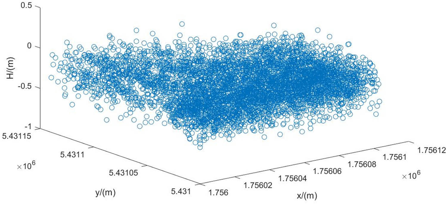
Data for Case 2.

As in Case 1, it is assumed to be influenced by both a multiplicative error with a standard deviation of 0.002 m and an additive error with a standard deviation of 0.15 m. Given that the correct or incorrect selection of the fitting formula impacts the coefficient of determination, only the MSE and MAE values (Table 2) and the Bland–Altman analysis plots (Figure 6) for the two algorithms are considered here.

Table 2

Accuracy statistics of the two algorithms (Case 2)

Algorithms	MSE (m)	MAE (m)
LS	0.0231	0.1213
BC	0.0225	0.1193

Figure 6

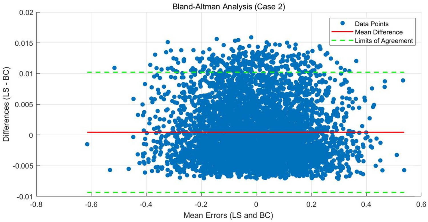
Bland–Altman analysis of LS and BC algorithms (Case 2).

As shown in Table 2, the MSE values are 0.0231 m for the LS method and 0.0225 m for the BC method, while the MAE values are 0.1213 m for the LS method and 0.1193 m for the BC method. The combined performance of both indices suggests that the BC method is slightly more accurate than the LS method. In comparison to the differences between the two algorithms in MSE and MAE in Case 1, the differences in Case 2 are much smaller. This is primarily because Case 1 is a mountainous area with significant changes in point cloud elevation, while the changes in point cloud elevation in Case 2 are minimal. Additionally, the influence of the multiplicative error is smaller, leading to reduced differences between the two error models.

In Figure 6, the mean difference value is 0.0004, and the limits of agreement are −0.0093 and 0.0102 (95%), which is calculated as 1.96 times the standard deviation. The mean difference line is close to 0, indicating that the two algorithms exhibit a very small average deviation overall. As shown in Figure 6, many data points still exceed the upper bound of consistency, indicating that, despite the small mean deviation of the two algorithms, substantial differences exist for certain specific measurements. This finding is consistent with Case 1, as the mixed additive and multiplicative error is inherently different from the additive error.

Combining the results from Table 1, Figure 4, and Case 1, it can be concluded that the BC algorithm outperforms the LS method in terms of accuracy in both mountainous and flat areas, with a more pronounced accuracy advantage in mountainous areas characterized by large undulations.

3.3 Case 3

In actual production, influenced by ground features, the ground points obtained by filtering are not continuous; instead, they display areas of significant or minor gaps. At such times, interpolation of surrounding ground points is necessary to achieve completeness. The fundamental theory behind the interpolation method assumes that ground points in a region follow a specific functional distribution, which is used to derive the interpolation point information. Since actual measurement data invariably contain errors and their true values are indeterminable, simulated DTM data serve to verify that the mixed additive and multiplicative error model is superior for DTM interpolation compared to the additive error model. It is posited that the DTM data for a region strictly adhere to the following functional model:

(24) h ( x , y ) = 5 + 0.6 x + 0.8 y − 0.7 x y + 0.9 x 2 − 0.4 y 2

The horizontal and vertical coordinates were taken in the range of 1–100 m, in steps of 2 m. The real DTM data of the area were obtained, as shown in Figure 7:

Figure 7

DTM truth value.

It is posited that the DTM for the region, derived from LiDAR data, is influenced by multiplicative errors with a mean of 0 and a standard deviation of 0.3 m, and by additive errors with a standard deviation of 1.5 m. The DTM derived from LiDAR data is depicted in Figure 8:

Figure 8

DTM disturbed by noise.

Figure 8 illustrates the simulated DTM affected by a combination of multiplicative and additive errors. Compared to the real DTM in Figure 7, the DTM error reaches a maximum of 5,000 m. As shown in Figure 8, the basic characteristics of multiplicative error are evident: as the DTM value increases, the observation error also increases, which fundamentally differs from the traditional additive error model.

It is assumed that points with horizontal and vertical coordinates ranging from 51 to 71 m are feature points which have been filtered out, creating a gap. The corresponding measured data are depicted in Figure 9:

Figure 9

DTM after filtering.

Points within the ellipse in Figure 9 represent gaps resulting from the exclusion of feature points, which require interpolation from the existing data. Interpolation is now performed using the least-squares method based on additive error theory and the method employing a mixed additive and multiplicative error model, respectively. The accuracies of these two algorithms in this region are presented in Table 3.

Table 3

Comparison of the interpolation accuracy of the two algorithms

Algorithms	MSE (m)	MAE (m)
LS	1032.7296	31.8203
BC	336.2205	17.2087

From Table 3, the MSE and MAE values for the BC method are lower than those for the LS method, demonstrating the superior overall accuracy of the BC method’s interpolation. This also suggests that the mixed additive–multiplicative error model is more effective for DTM interpolation than the purely additive error model. The regression coefficients calculated by the two algorithms are presented in Table 4:

Table 4

Regression coefficients for the two algorithms

Algorithms	β 1	β 2	β 3	β 4	β 5	β 6
Truth value	5	0.6	0.8	−0.7	0.9	0.4
LS	33.6850	0.3118	−1.6588	−0.7169	0.9112	0.4340
BC	5.4462	0.3107	0.7710	−0.7035	0.8968	0.4069

Comparing the regression coefficients with the true values in Table 4, it is evident that the coefficients obtained by the BC method more closely align with reality. Synthesizing the results from the three case studies, the BC method, which utilizes the mixed additive and multiplicative error model, demonstrates greater accuracy than the LS method, which relies on the additive error model in both overall DTM fitting and interpolation. This suggests that for processing LiDAR data to obtain DTM, employing the mixed additive and multiplicative error model ensures greater accuracy.

4 Conclusion

When utilizing LiDAR data to obtain DTMs, the current methods predominantly rely on additive error theory. However, it has been established that LiDAR data are influenced by both multiplicative and additive errors, which also affect the resulting DTMs. In the field of geodesy, Xu et al. [28] proposed a mixed additive and multiplicative error model, which we applied to the generation of DTM products using LiDAR data. Following a case study, we reached the following conclusions:

In mountainous regions characterized by significant topographic variation, the LS method yields a mean squared error of 6.2524 m, whereas the BC method yields 4.0660 m. Regarding the mean absolute error, the LS method produces a value of 2.0063 m, while the BC method produces 1.5991 m. In the R ² index, the LS method achieves 0.7980, whereas the BC method achieves 0.8621. Collectively, these three metrics demonstrate that the BC method outperforms the LS method in regions with complex terrain.
In flat terrain regions, the LS method yields a mean squared error of 0.0231 m, while the BC method yields 0.0225 m. Regarding the mean absolute error, the LS method produces a value of 0.1213 m, whereas the BC method produces 0.1193 m. Based on the performance of these two metrics, the BC method demonstrates marginally superior accuracy compared to the LS method.
Whether in mountainous or flat terrain, Bland–Altman plots reveal fundamental differences between the two error models.
For DTM interpolation, the LS method yields a mean squared error of 1032.7296 m, whereas the BC method yields 336.2205 m. Regarding the mean absolute error, the LS method produces a value of 31.8203 m, while the BC method produces 17.2087 m. Moreover, the regression coefficients obtained through the BC method are more consistent with real-world conditions.

Acknowledgments

The authors gratefully acknowledge anonymous reviewers for their thorough reading of this manuscript and for their insightful questions and constructive suggestions, which significantly improved the quality of this article.

Funding information: This manuscript was supported by the National Natural Science Foundation of China (No. 41674013).
Author contributions: Conceptualization: Guohong Li; methodology: Guohong Li; programming: Xiaohui Song and Khan Rehan; data curation: Huijuan Xin and Guohong Li; writing original draft preparation: Guohong Li; and writing review and editing: Guohong Li and Khan Rehan. All authors have read and agreed to the published version of the manuscript.
Conflict of interest: The authors declare that there are no conflicts of interest.
Data availability statement: Some or all data, or code generated or used during the study are available from the corresponding author by reasonable request.

References

[1] Flamant PH, Menzies RT, Kavaya MJ. Evidence for speckle effects on pulsed CO2 lidar signal returns from remote targets. Appl Opt. 1984;23(9):1412–7.10.1364/AO.23.001412Search in Google Scholar

[2] Wang JY, Pruitt PA. Effects of speckle on the range precision of a scanning lidar. Appl Opt. 1992;31(6):801–8.10.1364/AO.31.000801Search in Google Scholar PubMed

[3] Hill C, Harris M, Ridley K, Jakeman E, Lutzmann P. Lidar frequency modulation barometers in the presence of speckle. Appl Opt. 2003;42(6):1091–100.10.1364/AO.42.001091Search in Google Scholar

[4] Zhou S, Fan L, Xiang J, Sun J. Island’s DTM generating method based on LIDAR point cloud. J Shandong Univ Sci Technol. 2015;34(3):53–61 (In Chinese).Search in Google Scholar

[5] Zhang K, Chen SC, Whitman D, Shyu ML, Yan J, Zhang C. A progressive morphological filter for removing non ground measurements from air-borne LIDAR data. IEEE Trans Geosci Remote Sens. 2003;41(4):872–82.10.1109/TGRS.2003.810682Search in Google Scholar

[6] Chen Q, Gong P, Baldocchi D, Xie G. Filtering airborne laser scanning data with morphological methods. Photogramm Eng Remote Sens. 2007;73(2):175–85.10.14358/PERS.73.2.175Search in Google Scholar

[7] Meng X, Wang L, Silván-Cárdenas JL, Currit N. A multi-directional ground filtering algorithm for airborne LIDAR. ISPRS J Photogramm Remote Sens. 2009;64(1):117–24.10.1016/j.isprsjprs.2008.09.001Search in Google Scholar

[8] Sithole G, Vosselman G. Experimental comparison of filter algorithms for bare-Earth extraction from airborne laser scanning point clouds. ISPRS J Photogramm Remote Sens. 2004;59(1):85–101.10.1016/j.isprsjprs.2004.05.004Search in Google Scholar

[9] Li Y, Wu H. Filtering airborne LIDAR data based on morphological gradient. J Remote Sens. 2008;12(4):633–9 (In Chinese).Search in Google Scholar

[10] Mongus D, Žalik B. Parameter-free ground filtering of LiDAR data for automatic DTM generation. ISPRS J Photogramm Remote Sens. 2012;67(1):1–12.10.1016/j.isprsjprs.2011.10.002Search in Google Scholar

[11] Maguya AS, Junttila V, Kauranne T. Adaptive algorithm for large scale DTM interpolation from LIDAR data for forestry applications in steep forested terrain. ISPRS J Photogramm Remote Sens. 2013;85:74–83.10.1016/j.isprsjprs.2013.08.005Search in Google Scholar

[12] Xiong J, Fang Y, Deng D. Surface fitting filtering based on least square method from LiDAR data. Sci Surv Mapp. 2013;38(4):74–6 (In Chinese).Search in Google Scholar

[13] Chen J. Terrain feature extraction based on airborne LiDAR point cloud data. Guilin, Guangxi: Guilin University of Technology; 2023 (In Chinese: Master’s Degree Thesis).Search in Google Scholar

[14] Gillin CP, Bailey SW, McGuire KJ, Prisley SP. Evaluation of LiDAR-derived DEMs through terrain analysis and field comparison. Photogramm Eng Remote Sens. 2015;81(5):387–96.10.14358/PERS.81.5.387Search in Google Scholar

[15] Contreras MA, Staats W, Yiang J, Parrott D. Quantifying the accuracy of LiDAR-derived DEM in deciduous eastern forests of the Cumberland Plateau. J Geogr Inf Syst. 2017;9(3):339–53.10.4236/jgis.2017.93021Search in Google Scholar

[16] Sibona E, Vitali A, Meloni F, Caffo L, Dotta A, Lingua E, et al. Direct measurement of tree height provides different results on the assessment of LiDAR accuracy. Forests. 2016;8(1):7–20.10.3390/f8010007Search in Google Scholar

[17] Guerra-Hernández J, Cosenza DN, Rodriguez LCE, Silva M, Tomé M, Díaz-Varela RA, et al. Comparison of ALS-and UAV (SfM)-derived high-density point clouds for individual tree detection in Eucalyptus plantations. Int J Remote Sens. 2018;39(15–16):5211–35.10.1080/01431161.2018.1486519Search in Google Scholar

[18] Kovanič Ľ, Blistan P, Urban R, Štroner M, Blišťanová M, Bartoš K, et al. Analysis of the suitability of high-resolution DEM obtained using ALS and UAS (SfM) for the identification of changes and monitoring the development of selected geohazards in the alpine environment—A case study in high Tatras, Slovakia. Remote Sens. 2020;12(23):3901–18.10.3390/rs12233901Search in Google Scholar

[19] Cățeanu M, Ciubotaru A. Accuracy of ground surface interpolation from airborne laser scanning (ALS) data in dense forest cover. ISPRS Int J Geo-Inf. 2020;9(4):224.10.3390/ijgi9040224Search in Google Scholar

[20] Eren M, Hoşbaş RG. Testing the performance of the video camera to monitor the vertical movements of the structure via a specially designed steel beam apparatus. Meas Sci Rev. 2023;23(1):32–9.10.2478/msr-2023-0004Search in Google Scholar

[21] Erkoç MH, Doğan U. Machine learning models applied to altimetry era tide gauge and grid altimetry data for comparative long-term trend estimation: A study from Shikoku Island, Japan. Appl Ocean Res. 2024;150:104132.10.1016/j.apor.2024.104132Search in Google Scholar

[22] Tun SH, Changnv Z, Jamil F. GIS-based landslide susceptibility assessment using random forest and support vector machine models: A case study of Chin state, Myanmar. Acta Geodyn Geomater. 2024;21(3):207–40.10.13168/AGG.2024.0019Search in Google Scholar

[23] Kraus K, Pfeifer N. Determination of terrain models in wooded areas with airborne laser scanner data. ISPRS J Photogramm Remote Sens. 1998;53:193–203.10.1016/S0924-2716(98)00009-4Search in Google Scholar

[24] Kobler A, Pfeifer N, Ogrinc P, Todorovski L, Oštir K, Džeroski S. Repetitive interpolation: A robust algorithm for DTM generation from Aerial Laser Scanner Data in forested terrain. Remote Sens Environ. 2007;108:9–23.10.1016/j.rse.2006.10.013Search in Google Scholar

[25] Xu P, Shimada S. Least squares parameter estimation in multiplicative noise models. Commun Stat-Simul Comput. 2000;29(1):83–96.10.1080/03610910008813603Search in Google Scholar

[26] Ewing C, Mitchell M. Introduction to geodesy. New York: Elsevier; 1970.Search in Google Scholar

[27] Seeber G. Satellite Geodesy. 2nd edn. Berlin: de Gruyter; 2003.10.1515/9783110200089Search in Google Scholar

[28] Xu P, Shi Y, Peng J, Liu J, Shi C. Adjustment of geodetic measurements with mixed multiplicative and additive random errors. J Geodesy. 2013;87(7):629–43.10.1007/s00190-013-0635-2Search in Google Scholar

[29] Magnus J, Neudecker H. Matrix differential calculus with applications in statistics and econometrics. New York: Wiley; 1988.10.2307/2531754Search in Google Scholar

[30] McCullagh P. Quasi-likelihood functions. Ann Stat. 1983;11:59–67.10.1214/aos/1176346056Search in Google Scholar

[31] McCullagh P, Nelder J. Generalized linear models. 2nd edn. London: Chapman and Hall; 1989.10.1007/978-1-4899-3242-6Search in Google Scholar

[32] Dennis J, Schnabel R. Numerical methods for unconstrained optimization and nonlinear equations. In SIAM classics in applied mathematics, Philadelphia. Englewood Cliffs, New Jersey: Prentice-Hall, Inc.; 1983.Search in Google Scholar

[33] Wang L, Chen T. Virtual observation iteration solution and A-optimal design method for ill-posed mixed additive and multiplicative random error model in geodetic measurement. J Surv Eng. 2021;147(4):04021016.10.1061/(ASCE)SU.1943-5428.0000363Search in Google Scholar

[34] Wang L, Chen T. The SUT method for precision estimation of mixed additive and multiplicative random error model. Acta Geod Cartogr Sin. 2022;51(11):2303–16 (In Chinese).Search in Google Scholar

[35] Wang L, Chen T, Zhou C. Weighted least squares regularization iteration solution and precision estimation for ill-posed multiplicative error model. Acta Geod Cartogr Sin. 2021;50(5):589–99 (In Chinese).Search in Google Scholar

[36] Shi Y. Least squares parameter estimation in additive/multiplicative error models for use in geodesy. Geomat Inf Sci Wuhan Univ. 2014;39(9):1033–7 (In Chinese).Search in Google Scholar

[37] Shi Y, Xu P, Peng J, Shi C, Liu J. Adjustment of measurements with multiplicative errors: error analysis，estimates of the variance of unit weight, and effect on volume estimation from LiDAR-type digital elevation models. Sensors (Basel, Switzerland). 2014;14(1):1249–66.10.3390/s140101249Search in Google Scholar PubMed PubMed Central

Received: 2024-11-12

Revised: 2025-04-16

Accepted: 2025-04-18

Published Online: 2025-05-28

This work is licensed under the Creative Commons Attribution 4.0 International License.

Articles in the same Issue

https://doi.org/10.1515/geo-2025-0809

Keywords for this article

digital terrain model; mixed additive and multiplicative random errors model; additive errors; LiDAR

Creative Commons

BY 4.0