Comparison of several seismic active earth pressure calculation methods for retaining structures
-
Xin Huang
 ,
Jingshan Bo
,
Jingshan Bo

Abstract
Earthquake earth pressure is one of the key parameters for the seismic design of retaining structures. In this work, the seismic earth pressure calculation methods used in the design specifications of retaining walls, bridge abutments, and other retaining structures in various countries are summarized. Moreover, different calculation methods and examples are analysed and compared. A comparison shows that most of the specifications used or modified the M-O method for calculating seismic active earth pressure, and the calculation approach is basically consistent. The difference in the seismic active earth pressure at the bottom of the retaining walls calculated with various specifications gradually increases with increasing seismic peak acceleration. The coefficient of seismic active earth pressure and the resultant force of seismic active earth pressure both increase with increasing seismic peak acceleration. The calculation method, which considers the additional load at the top, results in a seismic earth pressure resultant force point at a height of above 1/3H. When calculating the seismic active earth pressure of reinforced soil structures under various specifications, the effect of reinforcement materials on the reduction in wall back earth pressure is not considered, and the calculation results are relatively conservative. The comparison results can provide a reference for the optimization and improvement of the seismic design of retaining structures, such as reinforced earth retaining walls.
1 Introduction
In the design of seismic stability in internal and external retaining structures, the calculation of the seismic active earth pressure on the wall back is considered a core component of structural strength verification. Scholars from various countries have conducted extensive research on the seismic earth pressure of retaining structures, employing five primary methods: limit equilibrium analysis, limit displacement theory, pseudodynamic research, finite element analysis, and experimental research. The limit equilibrium method is a quasistatic calculation method. Owing to its simplicity, clear physical significance, and small computational workload, this method is widely used in practice.
On the basis of the Coulomb earth pressure theory, Japanese scholars Mononobe and Matsuo [1] and Okabe [2] proposed the Mononobe–Okabe (M-O) method for calculating the active earth pressure on the back of retaining structure walls. In essence, this method is a quasistatic method that considers the horizontal and vertical seismic acceleration. This method has the following shortcomings according to Wu [3]: (1) the horizontal magnification factor of the retaining walls along the height direction is not considered; (2) the influence of the horizontal seismic inertia of the retaining wall is ignored; (3) the method is only applicable to cohesionless soil as the filler behind the wall without considering the cohesion of the filler; and (4) the acting point of the seismic earth pressure resultant force is considered to be located at 1/3 the height of the retaining wall. Seed and Whitman [4] modified the M-O method to obtain the seismic earth pressure through the peak acceleration of ground motion and the internal friction angle of fill. Sherif and Fang [5] considered the influence of wall rotation on earth pressure of retaining walls and demonstrated the accuracy of the – M-O method. In the study of highway abutment by Li [6], a formula for calculating seismic earth pressure by the horizontal seismic coefficient was derived to eliminate the seismic angle. Liang [7] overcame the drawbacks of the M-O method (requiring the seismic angle to be less than the friction angle) by studying the characteristics of the earth pressure error and railway load when the wall back inclination is large, and the scholars derived a new formula. Zhao [8] reported the corresponding calculation formula of earth pressure for cohesionless soil and cohesive soil. Chen et al. [9] derived the generalized physical part of the M-O calculation formula and applied it to the cohesive soil retaining walls through the re-exploration and research of the generalized Coulomb theory. Wang et al. [10] proposed the calculation model for the seismic active earth pressure that considers time and phase changes for cohesive soil and cohesionless soil, respectively, on the basis of the pseudodynamic method. Zhang and Song [11] investigated the earth pressure coefficient with the strain increment ratio on the basis of the law of change. They proposed a practical calculation method in which the seismic earth pressure can be considered the lateral deformation of fill. The reasonableness of the method was verified through the earth pressure model test results. Yang et al. [12] deduced the seismic earth pressure calculation formula for reinforced gravity retaining walls according to the force polygon method. Zhou et al. [13] considered the effects of the rotation of the principal stresses, time effects, and wall–back inclination, and derived a new solution for the seismic active failure angle by the pseudodynamic method, according to the total force equilibrium of the sliding soil mass. Through a horizontal differential layer method, new differential equations of the normal seismic active earth pressure and the coefficient for an inclined rigid retaining wall were obtained while considering translation. Yu [14], on the basis of the upper bound method of plastic limit analysis and the quasistatic method, adopted a logarithmic spiral surface as the slip surface, and established a calculation method for the seismic earth pressure of the reinforced gravity wall. Wang et al. [15] established a calculation method for the active earth pressure of unsaturated fill under earthquake action for gravity retaining walls on the basis of the upper bound principle of limit analysis. Du et al. [16] proposed two calculation methods for the earth pressure of gravity reinforced earth retaining walls under different reinforcement strength and pressure conditions on the basis of the quasicohesion method and working stress principle of reinforced earth. Li et al. [17,18] deduced a calculation method for the seismic active earth pressure considering the displacement modes of reinforced earth retaining walls on the basis of the force polygon method and Winkler foundation beam model, and analysed the influences of different panel forms on the seismic earth pressure distributions of reinforced earth retaining walls.
Owing to different project types and industries, the calculation methods of seismic earth pressure vary in the seismic design specifications for various retaining structures in different countries. In this work, the calculation methods of seismic earth pressure in seismic design specifications of several common types of retaining structures are discussed, and the calculation results of the seismic earth pressure of retaining walls under different seismic loads in retaining wall structures with overlying loads are compared and analysed.
2 Calculation method of seismic earth pressure
2.1 M-O method
The M-O method was proposed by Japanese scholars Mononobe and Okabe in 1924 to calculate the active earth pressure at the back of the retaining structure wall on the basis of the Coulomb earth pressure theory. In essence, this method is a quasistatic method considering the horizontal and vertical seismic acceleration. This method has four basic assumptions: (1) The fill behind the wall is homogeneous and cohesionless and composed of unsaturated soil, and the internal friction angle of the fill is a fixed value. (2) The retaining wall can produce enough lateral displacement to yield the filling at the back of the wall with a shear sliding fracture surface. (3) At this time, the earth pressure acting on the back of the wall is the minimum. (4) The fracture surface is the plane passing through the heel of the wall. The retaining wall is in plane plane-strain state.
The calculation formulas of seismic active earth pressure E ea and active earth pressure coefficient K ea obtained from limit equilibrium conditions and Coulomb earth pressure theory are as follows.
where γ is the gravity of soil mass, H is the height of the retaining wall, K h is the horizontal acceleration coefficient, K v is the vertical acceleration coefficient, θ is the seismic angle, φ is the internal friction angle of the soil, δ is the friction angle between the wall and soil, α is the angle between the retaining wall and the vertical direction, and β is the angle between the fill and horizontal direction. The stress of the sliding soil wedge behind the wall is shown in Figure 1.
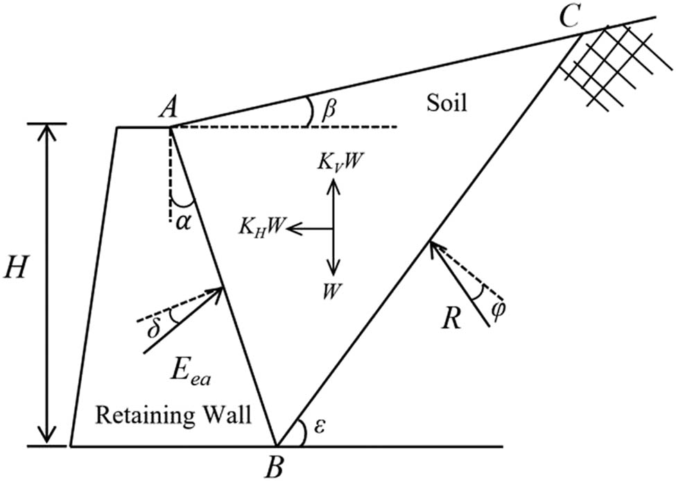
Schematic diagram of the force on the sliding soil wedge behind the wall.
2.2 Guidelines for seismic design of highway bridges (JTG/T B02-01-2008) [19]
This code is a standard for the highway engineering industry. The calculation of the seismic dynamic earth pressure at the back of the abutment wall in this code considers the cohesion of the fill, the adhesion on the contact surface between the abutment and soil at the back of the wall, and the uniformly distributed load on the sliding soil wedge. The calculation formula is derived on the basis of the M-O formula. The specific formulas of the seismic active earth pressure E ea and active earth pressure coefficient K a are as follows:
where γ is the filling weight, H is the height of the abutment retaining wall, q is the uniformly distributed load on the sliding soil wedge, α is the angle between the retaining wall and the vertical direction, β is the angle between the filling surface and the horizontal plane, c is the cohesion of the cohesive fill, δ is the friction angle between the wall and soil, θ is the seismic angle, φ is the internal friction angle of the soil, and K ca is the cohesive earth pressure coefficient of the fill. When the overlying load is q = 0, the location of the action point of seismic earth pressure can be taken as H/3 from the bottom of the abutment. When q ≠ 0, the position of the seismic earth pressure action point is H/3 plus the fill height converted by q. The calculation diagram is shown in Figure 2.
![Figure 2
Schematic diagram of the seismic active earth pressure calculation (JTG/T B02-01-2008) [19].](/document/doi/10.1515/geo-2025-0829/asset/graphic/j_geo-2025-0829_fig_002.jpg)
Schematic diagram of the seismic active earth pressure calculation (JTG/T B02-01-2008) [19].
When the filling behind the abutment is cohesionless soil, the following simplified formula can be used to calculate the seismic active earth pressure E ea and the active earth pressure coefficient K a :
where C i is the seismic importance coefficient, A is the peak horizontal seismic acceleration design, and g is the acceleration due to gravity. The action point of the seismic active earth pressure is 0.4H away from the abutment bottom.
2.3 Code for seismic design of railway engineering (2009) (GB 50111-2006) [20]
This code is a railway engineering industry standard, which stipulates that in the seismic design of bridge abutments, the seismic action of bridge abutments shall be calculated using the static method according to the design earthquake, and the seismic active earth pressure acting on the back of the abutment is calculated according to Coulomb’s theory. However, the gravity γ of the fill, the internal friction angle φ of the fill, and the friction angle δ between the wall soil and the back of the wall should be corrected by the seismic angle θ in the Coulomb formula before calculation, according to the influence of the seismic action. The seismic active earth pressure E ea , active earth pressure coefficient K a , and parameter correction formula of the abutment are as follows:
where γ E is the corrected filling weight, H is the height of the abutment retaining wall, α is the angle between the retaining wall and the vertical direction, β is the angle between the surface of the filled soil and the horizontal plane, φ E is the corrected internal friction angle of the filled soil, δ E is the corrected friction angle between the wall and the soil behind the wall, and θ is the seismic angle. The action point of the seismic active earth pressure is H/3 away from the abutment bottom.
2.4 Code for seismic design of urban bridges (CJJ166-2011) [21]
This code is a standard for the urban construction industry. The code considers that, in general, only horizontal seismic actions can be considered for urban bridge structures, and seismic actions along and across the bridge can be considered for straight-line bridges. The formulas for calculating the active earth pressure E ea and the active earth pressure coefficient K a of the abutment back under earthquake loading are as follows:
where γ is the filling weight, H is the height of the abutment retaining wall, A is the peak value of the horizontal design ground motion acceleration, φ is the internal friction angle of the soil, and g is the acceleration due to gravity. The action point of the seismic active earth pressure is 0.4H away from the bottom of the abutment.
Compared with the calculation method of the guidelines for seismic design of highway bridges (JTG/T B02-01-2008), the calculation method of seismic active earth pressure in this code ignores the seismic importance coefficient of the abutment, and does not consider the nature of the fill, the fill and wall back angle, the top load, etc. It belongs to a simplified calculation method.
2.5 Code for design of highway reinforced earth engineering (JTJ 015-91) [22]
This code is specifically applicable to highway reinforced soil slopes, reinforced soil embankments, etc. When calculating the seismic active earth pressure in the code, the structural importance of different highway grades, reinforced soil structure types, and horizontal seismic coefficients under different intensities is considered. The specific formulas of the seismic active earth pressure E ea and active earth pressure coefficient K a are as follows:
where γ is the filling weight, H is the height of the abutment retaining wall, C i is the structural importance correction coefficient of the highway grade, C Z is the comprehensive influence coefficient of the structure type, K h is the horizontal seismic coefficient, and φ is the internal friction angle of the soil. The action point of the seismic active earth pressure is 0.4H away from the bottom of the abutment.
In addition, when the filling surface at the back of the wall is an embankment slope, the unit weight γ, the internal friction angle φ, and the friction angle δ of the filling in (16) and (17) should be corrected according to the seismic angle. The specific correction formulas are as follows.
where γ E is the corrected filling weight, φ E is the corrected internal friction angle of the fill, δ E is the friction angle between the wall and the soil at the back of the wall after correction, and θ is the seismic angle.
2.6 U.S. NCMA code (National Concrete Masonry Association, 2012) [23]
The code provides an analysis and design method for ensuring the stability of segmental retaining walls (SRW) under seismic loads. The M-O method is used to calculate the seismic dynamic earth pressure in the seismic design. The horizontal and vertical accelerations are assumed to be constant in the face slab, reinforced area, and backfill area. The calculation formulas for the seismic active earth pressure E ea and active earth pressure coefficient K ea are as follows:
where γ is the filling weight, H is the height of the retaining wall, K h is the horizontal acceleration coefficient, K v is the vertical seismic acceleration coefficient, “+” corresponds to the downward seismic inertia force, “−” corresponds to the upward seismic inertia force, θ is the seismic angle, φ is the internal friction angle of the soil, ω is the angle between the retaining wall and the vertical direction, and is considered a positive value when the retaining wall is inclined in the filling direction at the back of the wall, δ is the friction angle between the wall and the soil, and β is the angle between the fill and the horizontal direction.
2.7 Design standards for railway structures are explained in the same way as those for retaining structures (2012) [24]
This code is a Japanese railway structure design standard applicable to retaining structures. The code provides a more comprehensive design method for reinforced earth retaining walls and reinforced earth abutments. In the code, the ground motion levels are divided into L1 and L2. L1 is the conventional earthquake that will inevitably occur within the design life of the structure, and L2 is the ground motion with a very low probability of occurrence but very high intensity within the design life of the structure. Compared with the Chinese seismic design specifications, L1 and L2 correspond to the design earthquake and rare earthquake in China, respectively [25].
The seismic active earth pressure (p AE) and active earth pressure coefficient (K AE ) of the reinforced earth abutment under the L1 ground motion level are calculated by the M-O method, and the calculation formulas are as follows.
where γ is the filling weight, H is the height of the retaining wall, q is the uniformly distributed load on the sliding soil wedge, α is the angle between the retaining wall and the vertical direction, β is the angle between the filling and the horizontal direction, φ is the internal friction angle of the soil, θ is the inclination angle between the resultant force and the vertical direction, δ is the friction angle between the wall and the soil, a max is the design ground motion peak acceleration, and g is the acceleration due to gravity. The action point of seismic active earth pressure is located at a height of H/3 from the bottom of the abutment.
During L2 ground motion, the dynamic characteristics (i.e. peak strength and residual strength) of the fill behind the wall after a strong earthquake are considered; thus, the M-O method is modified. The calculation formulas of the modified seismic active earth pressure coefficient K AE are as follows:
where ψ is the angle between the sliding surface and the horizontal plane. The meanings of other symbols are the same as above. Compared with the previous M-O method, the change in the earth pressure with increasing ground motion is more in line with field monitoring practices, and the active earth pressure during an earthquake can be reasonably calculated even for a large earthquake inertia force.
2.8 French code for design of reinforced soil (NF P 94-270, 2020) [26]
The calculation method of the seismic earth pressure of reinforced earth structure under seismic action in this code is also based on the M-O method, which is similar to the calculation method in the National Concrete Masonry Association code (NCMA, 2012). However, this code considers the influences of the top filling plane angle and horizontal displacement of the panel. The seismic active earth pressure E d and the active earth pressure coefficient K of the homogeneous soil layer can be calculated by the M-O method:
When
When
where γ is the filling weight, H is the height of the retaining wall, K
h
is the horizontal acceleration coefficient, K
v
is the vertical seismic acceleration coefficient, “+” corresponds to the downward seismic inertia force, “−” corresponds to the upward seismic inertia force, β is the angle between the filling and the horizontal direction,
2.9 Other specifications
In addition, the calculation methods for seismic dynamic earth pressure given in the specification of seismic design for highway engineering (JTG B02-2013) [27] and specifications for design of highway subgrades (JTG D30-2015) [28] are the same as those in the guidelines for seismic design of highway bridges (JTG/T B02-01-2008). In the local standard technical code for technical specifications for design and construction of flexible ecological reinforced earth retaining wall (DB33/T 988-2022) [29], the limit state design method is used to obtain the calculation method of active earth pressure to evaluate the external stability of reinforced retaining walls. However, the relevant provisions in the specification of seismic design for highway engineering (JTG B02-2013) are still used in the seismic design calculation, and the calculation method is the same as that in the guidelines for seismic design of highway bridges (JTG/T B02-01-2008).
3 Comparison of various calculation methods
The M-O method is generally used in the calculation of seismic earth pressure in various codes. However, some methods involve modifying the M-O formula according to the assumption considered, while keeping the calculation idea and process of seismic earth pressure basically the same. The objectives of these methods are as follows: (1) determine the importance coefficient of the project or structure; (2) determine the horizontal seismic influence coefficient and calculate the seismic angle; (3) determine the parameters in other earth pressure coefficients according to the design drawing of the retaining structure; (4) calculate the seismic earth pressure coefficient; and (5) calculate the value of the seismic dynamic earth pressure and determine the position of the resultant force action point. The differences between the calculation methods for seismic active earth pressure in the above specifications are shown in Table 1.
Comparison list of seismic active earth pressure calculation methods in various specifications
| Specification name | Considerations or assumptions |
|---|---|
| Code for highway engineering in China (JTG/T B02-01-2008, JTG B02-2013, JTG D30-2015, DB33T 988-2022) | The cohesion of the fill and the uniformly distributed load on the top of the fill are considered, but the horizontal seismic coefficient is not considered |
| Code for seismic design of railway engineering (2009) (GB 50111-2006) | The influence of earthquake action on the weight of the fill, the internal friction angle of the fill, and the friction angle between the wall and soil behind the wall is considered |
| Code for seismic design of urban bridges (CJJ166-2011) | The seismic importance coefficient of the abutment is ignored, and the nature of the fill and the horizontal seismic coefficient are not considered |
| Code for design of highway reinforced earth engineering (JTJ 015-91) | The structural importance of different highway grades, the type of reinforced earth structure, and whether the filling surface is an embankment slope are considered |
| Design manual for SRW (National Concrete Masonry Association, 2012) | It is assumed that the horizontal and vertical accelerations are constant in the face slab, reinforced area, and backfill area. That is, the acceleration amplification effect of the structure is ignored |
| Japanese railway standards, 2012 | The changes in the ground motion level and dynamic characteristics (peak strength and residual strength) of the fill are considered |
| French reinforced earth code (NF P 94-270, 2020) | The influences of the top filling plane angle and the horizontal displacement of the panel are considered |
To compare the practical application differences in seismic earth pressure calculation methods in the above specifications, a reinforced earth retaining wall structure with an overlying load is selected, and the calculation results of the seismic active earth pressure of the reinforced earth retaining wall under 0.1, 0.2, and 0.4g seismic peak accelerations are compared and analysed. The following conditions are assumed: (1) the back of the structural wall is vertical and smooth; (2) filling level is at the top of the reinforced earth retaining wall; (3) the project site is classified as class II site in Chinese specifications and class B site in European and American specifications; and (4) only horizontal seismic action is considered. The calculation diagram of the retaining wall is shown in Figure 3, and the structural design parameters are presented in Table 2.
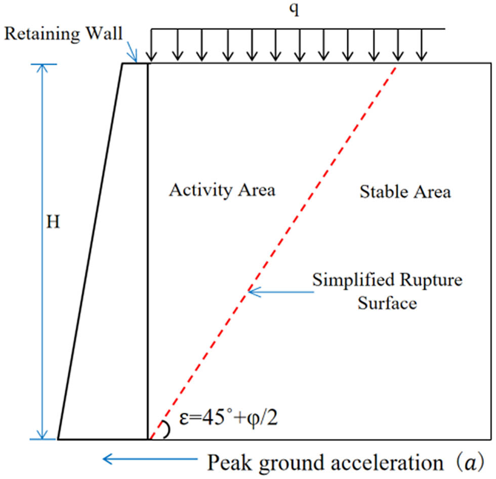
Calculation schematic diagram of the reinforced soil retaining wall calculation example.
Structural design parameters for the reinforced soil retaining wall calculation example
| Index | Parameter value |
|---|---|
| Type of fill behind the wall | Fine-gravel sand |
| Volume weight of the fill behind the wall γ (kN/m3) | 16.9 |
| Cohesion of fill behind the wall c (kPa) | 0 |
| Internal friction angle of the wall backfill φ (°) | 42 |
| Height of the wall H (m) | 4 |
| Overlying uniform load q (kPa) | 20 |
| Structural importance correction coefficient C i of highway grade | 0.8 |
| Comprehensive influence coefficient C Z of the structure type | 0.35 |
According to the seismic earth pressure calculation methods in the above specifications, the distribution curves of the seismic active earth pressure along the wall height of the reinforced earth retaining wall shown in this case can be obtained under the peak ground acceleration of 0.1, 0.2, and 0.4g under various calculation methods (Figure 4). The figures show that the seismic active earth pressure of each specification is linearly distributed along the wall height. The seismic active earth pressure value at the top of the wall in the Chinese highway bridge standard (JTG/T B02-01-2008) and Japanese railway standard (2012) is not zero. The greater the peak ground acceleration, the greater the difference. The seismic active earth pressure value at the top of the wall is zero according to the United States NCMA code (2012), the code for seismic design of railway engineering (2009) (GB 50111-2006), the code for design of highway reinforced earth engineering (JTJ 015-91), the code for seismic design of urban bridges (CJJ166-2011), and the French reinforced earth code (NF p94-270,2020). Under a seismic peak acceleration of 0.1g, the calculation results of the seismic active earth pressure of each method from small to large are the United States NCMA code (2012), the code for seismic design of railway engineering (2009) (GB 50111-2006), the code for design of highway reinforced earth engineering (JTJ 015-91), the code for seismic design of urban bridges (CJJ166-2011), the French reinforced earth code (NF p94-270,2020), the Japanese railway standards (2012), and the guidelines for seismic design of highway bridges (JTG/T B02-01-2008). At seismic peak accelerations of 0.2 and 0.4g, the calculation result of the seismic active earth pressure of the United States NCMA specification (2012) is greater than that of the code for seismic design of railway engineering (2009) (GB 50111-2006), and the calculation result of Japanese railway standards (2012) is greater than that of the guidelines for seismic design of highway bridges (JTG/T B02-01-2008). With increasing seismic peak acceleration, the difference in the seismic active earth pressure at the bottom of the wall calculated by various codes increases.
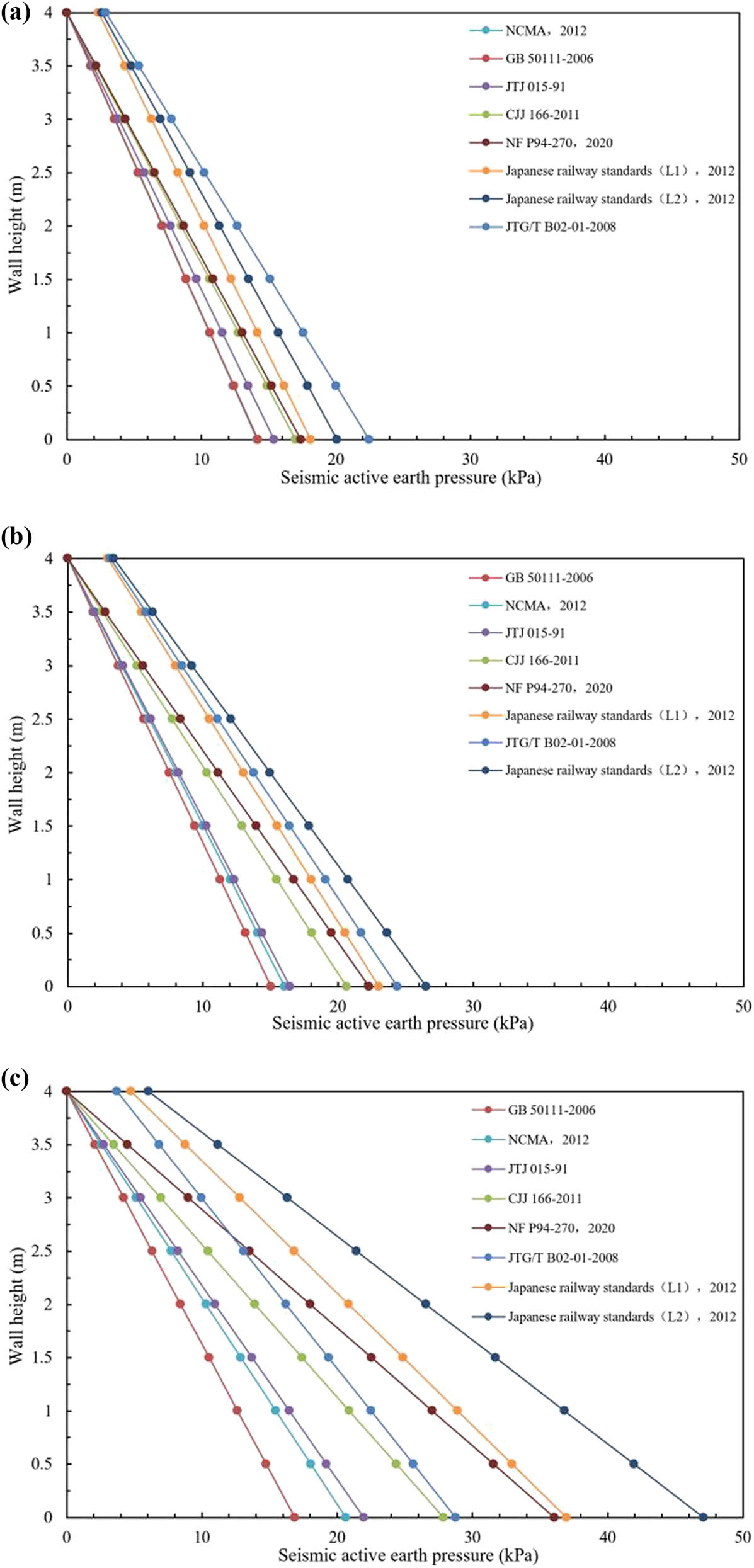
Seismic active earth pressure distribution curve along the wall height. (a) Seismic peak acceleration 0.1g. (b) Seismic peak acceleration 0.2g. (c) Seismic peak acceleration 0.4g.
According to the seismic active earth pressure calculation methods specified in the above codes, the seismic active earth pressure coefficient of the reinforced earth retaining wall shown in this case can be obtained under different peak ground accelerations. Then, based on the distribution curve of seismic active soil pressure along the wall height obtained from Figure 4, the magnitude and location of the resultant force of seismic active soil pressure under different peak accelerations can be plotted, as shown in Figure 5. The figures show that the seismic active earth pressure coefficients in the code for seismic design of urban bridges (CJJ166-2011) are the same under different seismic peak accelerations because the seismic active earth pressure coefficient calculation method in the code is related only to the internal friction angle of the fill, and the seismic active earth pressure coefficients obtained in other specifications increase with increasing ground motion acceleration. The seismic active earth pressure resultant force obtained in each code increases with increasing ground motion acceleration, and the calculation value in the guidelines for seismic design of highway bridges (JTG/T B02-01-2008) increases the fastest. The guidelines for seismic design of highway bridges (JTG/T B02-01-2008) and the Japanese railway standards (2012) both consider the additional load on the top when calculating the seismic earth pressure. Thus, the acting point of the seismic earth pressure resultant force is 0.37 of the wall height, which is higher than 1/3 of the wall height. The acting point of the seismic earth pressure resultant force calculated by other specifications is 1/3 of the wall height.
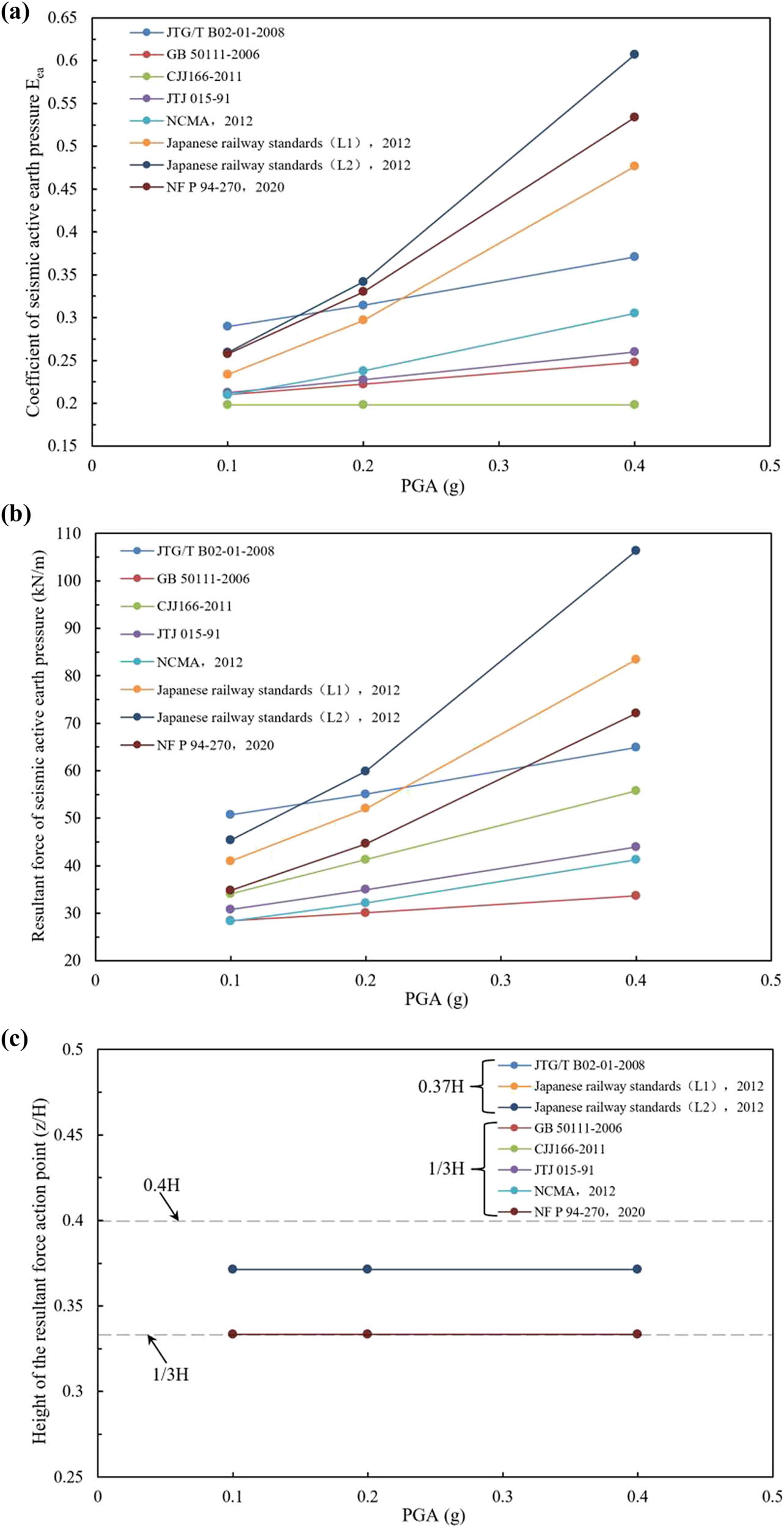
Relationship curve between the seismic active earth pressure resultant force and seismic motion during earthquakes. (a) Coefficient of seismic active earth pressure. (b) Resultant force of seismic active earth pressure. (c) Height of the resultant force action point.
4 Discussion
For reinforced earth retaining walls, the reduction effect of reinforcement on the seismic active earth pressure at the back of the wall is not considered in all specifications. However, many studies on the earth pressure of reinforced retaining walls [12,30,31,32] have shown that friction reinforcement is a main factor that reduces the earth pressure at the back of the retaining wall. Therefore, in theory, the calculation method of the seismic active earth pressure in this work can be considered conservative when applied to reinforced earth retaining walls.
5 Conclusions
The M-O method is essentially used in the calculation of seismic earth pressure in various codes. Conversely, the M-O formula is modified according to the assumption considered. However, the calculation idea and process of seismic earth pressure are basically the same.
In the comparison of calculation examples of retaining wall structures, the difference in the seismic active earth pressure at the bottom of the wall, according to calculations by various codes, gradually increases with increasing seismic peak acceleration. The coefficient of seismic active earth pressure and the resultant force of seismic active earth pressure obtained from each code increase with increasing ground motion acceleration. The guidelines for seismic design of highway bridges (JTG/T B02-01-2008) and the Japanese railway standards (2012) consider the additional load on the top. Therefore, the acting point of seismic earth pressure resultant force is at 0.37H, which is higher than 1/3H, while those of the other codes are at 1/3H.
In this work, only the theoretical calculations of various specifications are compared, but these results need to be further compared with large-scale model tests and specific seismic damage monitoring data from engineering projects. These comparisons will allow for the analysis of the applicability of the calculation methods of various specifications in specific engineering applications.
-
Funding information: This research was funded by the Fundamental Research Funds for the Central Universities, grant number ZY20215120, and the Earthquake Technology Spark Program of China, grant number XH23067YA.
-
Author contributions: Conceptualization, X.H. and X.C.; writing paper, Y.Q.; supervision, J.B.; resources, S.L. and Y.L. All authors have read and agreed to the published version of the manuscript.
-
Conflict of interest: The authors declare no conflict of interest.
-
Informed consent statement: All study participants provided informed consent.
-
Data availability statement: Data openly available in a public repository.
References
[1] Mononobe N, Matsuo H. On the determination of earth pressures during earthquakes. Proc World Eng Congr. 1929;9:192.Suche in Google Scholar
[2] Okabe S. General theory of earth pressure. J Jpn Soc Civ Eng. 1926;12(1):311.Suche in Google Scholar
[3] Wu XM. Study on soil pressure of abutment founded on piles and its influence factors under earthquake action. Chengdu: Southwest Jiaotong University; 2017. (in Chinese).Suche in Google Scholar
[4] Seed HB, Whitman RV. Design of earth retaining structures for dynamic loads. ASCE Specialty Conf. on Lateral Stresses in the Ground and Design of Earth Retaining Structures. Ithaca, NY: 1970. p. 103–47.Suche in Google Scholar
[5] Sherif MA, Fang YS. Dynamic earth pressure on walls rotating about the top. Soil Found. 1984;24(4):109–17.10.3208/sandf1972.24.4_109Suche in Google Scholar
[6] Li T. Simplified calculating formula for active earth pressure of earthquake expressed by earthquake coefficient method. J Railw Eng Soc. 1996;49(1):103–5. (in Chinese).Suche in Google Scholar
[7] Liang B. Simplified calculation method of active earth pressure on back of abutment under earthquake condition. J Railw Eng Soc. 1999;16(2):36–8. (in Chinese).Suche in Google Scholar
[8] Zhao MH. Soil mechanics and foundation engineering. Wuhan: Wuhan University of Technology Press; 2000. (in Chinese).Suche in Google Scholar
[9] Chen XL, Tao XX, Chen XM. Review of study on seismic response of gravity type retaining wall. J Nat Disasters. 2006;15(3):139–46. (in Chinese). 10.3969/j.issn.1004-4574.2006.03.024.Suche in Google Scholar
[10] Wang ZK, Xia TD, Chen WY. Pseudo-dynamic analysis for seismic active earth pressure behind rigid retaining wall. J Zhejiang Univ (Eng Sci). 2012;46(1):46–51. (in Chinese). 10.3785/j.issn.1008-973X.2012.01.08 Suche in Google Scholar
[11] Zhang JM, Song F. Evaluation of seismic earth pressure considering lateral deformation. China Earthq Eng J. 2013;35(1):9–20. (in Chinese). 10.3969/j.issn.1000-0844.2013.01.0009.Suche in Google Scholar
[12] Yang CW, Zhang JJ, Chen Q, Qu HL. Research on aseismic design of reinforced gravity retaining wall. China Civ Eng J. 2015;48(8):77–85. (in Chinese) 10.15951/j.tmgcxb.2015.08.009.Suche in Google Scholar
[13] Zhou YT, Chen FQ, Wang XM. Seismic active earth pressure for inclined rigid retaining walls considering rotation of the principal stresses with pseudo-dynamic method. Int J Geomech. 2018;18(7):04018083. 10.1061/(ASCE)GM.1943-5622.0001198.Suche in Google Scholar
[14] Yu XZ. Study on calculation method of seismic earth pressure on flexible tensioned gravity wall. Subgrade Eng. 2020;208(1):147–51. (in Chinese) 10.13379/j.issn.1003-8825.2020.01.29.Suche in Google Scholar
[15] Wang L, Chen GX, Feng JX, Huang AP, Xu MJ. Semi-analytical method for the limit analysis of active earth pressure of unsaturated soil under seismic action. China Earthq Eng J. 2022;44(6):1309–16+1421. (in Chinese). 10.20000/j.1000-0844.20220802003.Suche in Google Scholar
[16] Du HY, Song L, Liu J, Bai QY. Study on calculation method of earth pressure of gravity reinforced earth retaining wall. J Shihezi Univ (Natural Science). 2023;41(3):291–7. (in Chinese). 10.13880/j.cnki.65-1174/n.2022.21.036.Suche in Google Scholar
[17] Li SH, Cai XG, Xu HL, Feng JY, Huang X, Jing LP. Seismic active earth pressure analysis of modular⁃block reinforced soil retaining wall under RBT mode. J Basic Sci Eng. 2023;31(4):921–34. (in Chinese). 10.16058/j.issn.1005-0930.2023.04.010.Suche in Google Scholar
[18] Li SH, Cai XG, Wang XP, Xu HL, Huang X. Numerical simulation of the vibration responses of reinforced soil-retaining walls with different facings. China Earthq Eng J. 2024;46(1):163–73. (in Chinese). 10.20000/j.1000-0844.20220317002 Suche in Google Scholar
[19] JTG/T B02-01-2008. Guidelines for seismic design of highway bridges. Beijing: China Communications Press; 2008. (in Chinese).Suche in Google Scholar
[20] GB 50111-2006. Code for seismic design of railway engineering (2009). Beijing: China Planning Press; 2009. (in Chinese).Suche in Google Scholar
[21] CJJ 166-2011. Code for seismic design of urban bridges. Beijing: China Architecture& Building Press; 2011. (in Chinese).Suche in Google Scholar
[22] JTJ 015-91. Code for design of highway reinforced earth engineering. Beijing: China Communications Press; 1991. (in Chinese).Suche in Google Scholar
[23] National Concrete Masonry Association. Design manual for segmental retaining walls. 3rd edn. Virginia: National Concrete Masonry Association; 2012.Suche in Google Scholar
[24] Railway Comprehensive Technology Research Institute. Design standards for railway structures are explained in the same way as retaining structures. Tokyo: Maruyama Publishing House; 2012. (in Japanese).Suche in Google Scholar
[25] Weng Y, Zhu BL. Some comparisons between Chinese and Japanese code for earthquake resistance design of bridges. Sichuan Build Sci. 2010;36(3):161–4. (in Chinese). 10.3969/j.issn.1008-1933.2010.03.041.Suche in Google Scholar
[26] Association Française de Normalisation (AFNOR). Calculs géotechnique Ouvrages de soutènement Remblais renforcés et massifs en sol cloué, NF P 94-270. Norme française. 2020. (in French).Suche in Google Scholar
[27] JTG B02-2013. Specification of seismic design for highway engineering. Beijing: China Communications Press; 2013. (in Chinese).Suche in Google Scholar
[28] JTG D30-2015. Specif Des Highw subgrades. 2015. Beijing; China Communications Press. (in Chinese).Suche in Google Scholar
[29] DB33/T 988-2022. Technical specifications for design and construction of flexible ecological reinforced earth retaining wall. Zhejiang: China Communications Press; 2015. (in Chinese).Suche in Google Scholar
[30] Jiang CS. A theoretical analysis of geo-grids how to decrease the earth pressure acted on an embankment retaining structure. J Railw Eng Soc. 2007;(8):30–4. (in Chinese). 10.3969/j.issn.1006-2106.2007.08.009.Suche in Google Scholar
[31] Zhu HW, Yao LK, Zhang XH. Comparison of dynamic characteristics between netted and packaged reinforced soil retaining walls and recommendations for seismic design. Chin J Geotech Eng. 2012;34(11):2072–80 (in Chinese).Suche in Google Scholar
[32] Li LH, Zheng ZG, Yan H, Huang SP, Zhou XL. Analysis of earth pressure on geogrid reinforced retaining wall and improvement of its calculation method. J Northwest Polytech Univ. 2022;40(6):1366–74. (in Chinese). 10.3969/j.issn.1000-2758.2022.06.021.Suche in Google Scholar
© 2025 the author(s), published by De Gruyter
This work is licensed under the Creative Commons Attribution 4.0 International License.
Artikel in diesem Heft
- Research Articles
- Seismic response and damage model analysis of rocky slopes with weak interlayers
- Multi-scenario simulation and eco-environmental effect analysis of “Production–Living–Ecological space” based on PLUS model: A case study of Anyang City
- Remote sensing estimation of chlorophyll content in rape leaves in Weibei dryland region of China
- GIS-based frequency ratio and Shannon entropy modeling for landslide susceptibility mapping: A case study in Kundah Taluk, Nilgiris District, India
- Natural gas origin and accumulation of the Changxing–Feixianguan Formation in the Puguang area, China
- Spatial variations of shear-wave velocity anomaly derived from Love wave ambient noise seismic tomography along Lembang Fault (West Java, Indonesia)
- Evaluation of cumulative rainfall and rainfall event–duration threshold based on triggering and non-triggering rainfalls: Northern Thailand case
- Pixel and region-oriented classification of Sentinel-2 imagery to assess LULC dynamics and their climate impact in Nowshera, Pakistan
- The use of radar-optical remote sensing data and geographic information system–analytical hierarchy process–multicriteria decision analysis techniques for revealing groundwater recharge prospective zones in arid-semi arid lands
- Effect of pore throats on the reservoir quality of tight sandstone: A case study of the Yanchang Formation in the Zhidan area, Ordos Basin
- Hydroelectric simulation of the phreatic water response of mining cracked soil based on microbial solidification
- Spatial-temporal evolution of habitat quality in tropical monsoon climate region based on “pattern–process–quality” – a case study of Cambodia
- Early Permian to Middle Triassic Formation petroleum potentials of Sydney Basin, Australia: A geochemical analysis
- Micro-mechanism analysis of Zhongchuan loess liquefaction disaster induced by Jishishan M6.2 earthquake in 2023
- Prediction method of S-wave velocities in tight sandstone reservoirs – a case study of CO2 geological storage area in Ordos Basin
- Ecological restoration in valley area of semiarid region damaged by shallow buried coal seam mining
- Hydrocarbon-generating characteristics of Xujiahe coal-bearing source rocks in the continuous sedimentary environment of the Southwest Sichuan
- Hazard analysis of future surface displacements on active faults based on the recurrence interval of strong earthquakes
- Structural characterization of the Zalm district, West Saudi Arabia, using aeromagnetic data: An approach for gold mineral exploration
- Research on the variation in the Shields curve of silt initiation
- Reuse of agricultural drainage water and wastewater for crop irrigation in southeastern Algeria
- Assessing the effectiveness of utilizing low-cost inertial measurement unit sensors for producing as-built plans
- Analysis of the formation process of a natural fertilizer in the loess area
- Machine learning methods for landslide mapping studies: A comparative study of SVM and RF algorithms in the Oued Aoulai watershed (Morocco)
- Chemical dissolution and the source of salt efflorescence in weathering of sandstone cultural relics
- Molecular simulation of methane adsorption capacity in transitional shale – a case study of Longtan Formation shale in Southern Sichuan Basin, SW China
- Evolution characteristics of extreme maximum temperature events in Central China and adaptation strategies under different future warming scenarios
- Estimating Bowen ratio in local environment based on satellite imagery
- 3D fusion modeling of multi-scale geological structures based on subdivision-NURBS surfaces and stratigraphic sequence formalization
- Comparative analysis of machine learning algorithms in Google Earth Engine for urban land use dynamics in rapidly urbanizing South Asian cities
- Study on the mechanism of plant root influence on soil properties in expansive soil areas
- Simulation of seismic hazard parameters and earthquakes source mechanisms along the Red Sea rift, western Saudi Arabia
- Tectonics vs sedimentation in foredeep basins: A tale from the Oligo-Miocene Monte Falterona Formation (Northern Apennines, Italy)
- Investigation of landslide areas in Tokat-Almus road between Bakımlı-Almus by the PS-InSAR method (Türkiye)
- Predicting coastal variations in non-storm conditions with machine learning
- Cross-dimensional adaptivity research on a 3D earth observation data cube model
- Geochronology and geochemistry of late Paleozoic volcanic rocks in eastern Inner Mongolia and their geological significance
- Spatial and temporal evolution of land use and habitat quality in arid regions – a case of Northwest China
- Ground-penetrating radar imaging of subsurface karst features controlling water leakage across Wadi Namar dam, south Riyadh, Saudi Arabia
- Rayleigh wave dispersion inversion via modified sine cosine algorithm: Application to Hangzhou, China passive surface wave data
- Fractal insights into permeability control by pore structure in tight sandstone reservoirs, Heshui area, Ordos Basin
- Debris flow hazard characteristic and mitigation in Yusitong Gully, Hengduan Mountainous Region
- Research on community characteristics of vegetation restoration in hilly power engineering based on multi temporal remote sensing technology
- Identification of radial drainage networks based on topographic and geometric features
- Trace elements and melt inclusion in zircon within the Qunji porphyry Cu deposit: Application to the metallogenic potential of the reduced magma-hydrothermal system
- Pore, fracture characteristics and diagenetic evolution of medium-maturity marine shales from the Silurian Longmaxi Formation, NE Sichuan Basin, China
- Study of the earthquakes source parameters, site response, and path attenuation using P and S-waves spectral inversion, Aswan region, south Egypt
- Source of contamination and assessment of potential health risks of potentially toxic metal(loid)s in agricultural soil from Al Lith, Saudi Arabia
- Regional spatiotemporal evolution and influencing factors of rural construction areas in the Nanxi River Basin via GIS
- An efficient network for object detection in scale-imbalanced remote sensing images
- Effect of microscopic pore–throat structure heterogeneity on waterflooding seepage characteristics of tight sandstone reservoirs
- Environmental health risk assessment of Zn, Cd, Pb, Fe, and Co in coastal sediments of the southeastern Gulf of Aqaba
- A modified Hoek–Brown model considering softening effects and its applications
- Evaluation of engineering properties of soil for sustainable urban development
- The spatio-temporal characteristics and influencing factors of sustainable development in China’s provincial areas
- Application of a mixed additive and multiplicative random error model to generate DTM products from LiDAR data
- Gold vein mineralogy and oxygen isotopes of Wadi Abu Khusheiba, Jordan
- Prediction of surface deformation time series in closed mines based on LSTM and optimization algorithms
- 2D–3D Geological features collaborative identification of surrounding rock structural planes in hydraulic adit based on OC-AINet
- Spatiotemporal patterns and drivers of Chl-a in Chinese lakes between 1986 and 2023
- Land use classification through fusion of remote sensing images and multi-source data
- Nexus between renewable energy, technological innovation, and carbon dioxide emissions in Saudi Arabia
- Analysis of the spillover effects of green organic transformation on sustainable development in ethnic regions’ agriculture and animal husbandry
- Factors impacting spatial distribution of black and odorous water bodies in Hebei
- Large-scale shaking table tests on the liquefaction and deformation responses of an ultra-deep overburden
- Impacts of climate change and sea-level rise on the coastal geological environment of Quang Nam province, Vietnam
- Reservoir characterization and exploration potential of shale reservoir near denudation area: A case study of Ordovician–Silurian marine shale, China
- Seismic prediction of Permian volcanic rock reservoirs in Southwest Sichuan Basin
- Application of CBERS-04 IRS data to land surface temperature inversion: A case study based on Minqin arid area
- Geological characteristics and prospecting direction of Sanjiaoding gold mine in Saishiteng area
- Research on the deformation prediction model of surrounding rock based on SSA-VMD-GRU
- Geochronology, geochemical characteristics, and tectonic significance of the granites, Menghewula, Southern Great Xing’an range
- Hazard classification of active faults in Yunnan base on probabilistic seismic hazard assessment
- Characteristics analysis of hydrate reservoirs with different geological structures developed by vertical well depressurization
- Estimating the travel distance of channelized rock avalanches using genetic programming method
- Landscape preferences of hikers in Three Parallel Rivers Region and its adjacent regions by content analysis of user-generated photography
- New age constraints of the LGM onset in the Bohemian Forest – Central Europe
- Characteristics of geological evolution based on the multifractal singularity theory: A case study of Heyu granite and Mesozoic tectonics
- Soil water content and longitudinal microbiota distribution in disturbed areas of tower foundations of power transmission and transformation projects
- Oil accumulation process of the Kongdian reservoir in the deep subsag zone of the Cangdong Sag, Bohai Bay Basin, China
- Investigation of velocity profile in rock–ice avalanche by particle image velocimetry measurement
- Optimizing 3D seismic survey geometries using ray tracing and illumination modeling: A case study from Penobscot field
- Sedimentology of the Phra That and Pha Daeng Formations: A preliminary evaluation of geological CO2 storage potential in the Lampang Basin, Thailand
- Improved classification algorithm for hyperspectral remote sensing images based on the hybrid spectral network model
- Map analysis of soil erodibility rates and gully erosion sites in Anambra State, South Eastern Nigeria
- Identification and driving mechanism of land use conflict in China’s South-North transition zone: A case study of Huaihe River Basin
- Evaluation of the impact of land-use change on earthquake risk distribution in different periods: An empirical analysis from Sichuan Province
- A test site case study on the long-term behavior of geotextile tubes
- An experimental investigation into carbon dioxide flooding and rock dissolution in low-permeability reservoirs of the South China Sea
- Detection and semi-quantitative analysis of naphthenic acids in coal and gangue from mining areas in China
- Comparative effects of olivine and sand on KOH-treated clayey soil
- YOLO-MC: An algorithm for early forest fire recognition based on drone image
- Earthquake building damage classification based on full suite of Sentinel-1 features
- Potential landslide detection and influencing factors analysis in the upper Yellow River based on SBAS-InSAR technology
- Assessing green area changes in Najran City, Saudi Arabia (2013–2022) using hybrid deep learning techniques
- An advanced approach integrating methods to estimate hydraulic conductivity of different soil types supported by a machine learning model
- Hybrid methods for land use and land cover classification using remote sensing and combined spectral feature extraction: A case study of Najran City, KSA
- Streamlining digital elevation model construction from historical aerial photographs: The impact of reference elevation data on spatial accuracy
- Analysis of urban expansion patterns in the Yangtze River Delta based on the fusion impervious surfaces dataset
- A metaverse-based visual analysis approach for 3D reservoir models
- Late Quaternary record of 100 ka depositional cycles on the Larache shelf (NW Morocco)
- Integrated well-seismic analysis of sedimentary facies distribution: A case study from the Mesoproterozoic, Ordos Basin, China
- Study on the spatial equilibrium of cultural and tourism resources in Macao, China
- Urban road surface condition detecting and integrating based on the mobile sensing framework with multi-modal sensors
- Application of improved sine cosine algorithm with chaotic mapping and novel updating methods for joint inversion of resistivity and surface wave data
- The synergistic use of AHP and GIS to assess factors driving forest fire potential in a peat swamp forest in Thailand
- Dynamic response analysis and comprehensive evaluation of cement-improved aeolian sand roadbed
- Rock control on evolution of Khorat Cuesta, Khorat UNESCO Geopark, Northeastern Thailand
- Gradient response mechanism of carbon storage: Spatiotemporal analysis of economic-ecological dimensions based on hybrid machine learning
- Comparison of several seismic active earth pressure calculation methods for retaining structures
- Mantle dynamics and petrogenesis of Gomer basalts in the Northwestern Ethiopia: A geochemical perspective
- Study on ground deformation monitoring in Xiong’an New Area from 2021 to 2023 based on DS-InSAR
- Paleoenvironmental characteristics of continental shale and its significance to organic matter enrichment: Taking the fifth member of Xujiahe Formation in Tianfu area of Sichuan Basin as an example
- Equipping the integral approach with generalized least squares to reconstruct relict channel profile and its usage in the Shanxi Rift, northern China
- InSAR-driven landslide hazard assessment along highways in hilly regions: A case-based validation approach
- Attribution analysis of multi-temporal scale surface streamflow changes in the Ganjiang River based on a multi-temporal Budyko framework
- Maps analysis of Najran City, Saudi Arabia to enhance agricultural development using hybrid system of ANN and multi-CNN models
- Hybrid deep learning with a random forest system for sustainable agricultural land cover classification using DEM in Najran, Saudi Arabia
- Long-term evolution patterns of groundwater depth and lagged response to precipitation in a complex aquifer system: Insights from Huaibei Region, China
- Remote sensing and machine learning for lithology and mineral detection in NW, Pakistan
- Spatial–temporal variations of NO2 pollution in Shandong Province based on Sentinel-5P satellite data and influencing factors
- Numerical modeling of geothermal energy piles with sensitivity and parameter variation analysis of a case study
- Stability analysis of valley-type upstream tailings dams using a 3D model
- Variation characteristics and attribution analysis of actual evaporation at monthly time scale from 1982 to 2019 in Jialing River Basin, China
- Investigating machine learning and statistical approaches for landslide susceptibility mapping in Minfeng County, Xinjiang
- Investigating spatiotemporal patterns for comprehensive accessibility of service facilities by location-based service data in Nanjing (2016–2022)
- A pre-treatment method for particle size analysis of fine-grained sedimentary rocks, Bohai Bay Basin, China
- Study on the formation mechanism of the hard-shell layer of liquefied silty soil
- Comprehensive analysis of agricultural CEE: Efficiency assessment, mechanism identification, and policy response – A case study of Anhui Province
- Simulation study on the damage and failure mechanism of the surrounding rock in sanded dolomite tunnels
- Towards carbon neutrality: Spatiotemporal evolution and key influences on agricultural ecological efficiency in Northwest China
- High-frequency cycles drive the cyclical enrichment of oil in porous carbonate reservoirs: A case study of the Khasib Formation in E Oilfield, Mesopotamian Basin, Iraq
- Reconstruction of digital core models of granular rocks using mathematical morphology
- Spatial–temporal differentiation law of habitat quality and its driving mechanism in the typical plateau areas of the Loess Plateau in the recent 30 years
- A machine-learning-based approach to predict potential oil sites: Conceptual framework and experimental evaluation
- Effects of landscape pattern change on waterbird diversity in Xianghai Nature Reserve
- Research on intelligent classification method of highway tunnel surrounding rock classification based on parameters while drilling
- River morphology and tectono-sedimentary analysis of a shallow river delta: A case study of Putaohua oil layer in Saertu oilfield (L. Cretaceous), China
- Review Articles
- Humic substances influence on the distribution of dissolved iron in seawater: A review of electrochemical methods and other techniques
- Applications of physics-informed neural networks in geosciences: From basic seismology to comprehensive environmental studies
- Ore-controlling structures of granite-related uranium deposits in South China: A review
- Shallow geological structure features in Balikpapan Bay East Kalimantan Province – Indonesia
- A review on the tectonic affinity of microcontinents and evolution of the Proto-Tethys Ocean in Northeastern Tibet
- Advancements in machine learning applications for mineral prospecting and geophysical inversion: A review
- Special Issue: Natural Resources and Environmental Risks: Towards a Sustainable Future - Part II
- Depopulation in the Visok micro-region: Toward demographic and economic revitalization
- Special Issue: Geospatial and Environmental Dynamics - Part II
- Advancing urban sustainability: Applying GIS technologies to assess SDG indicators – a case study of Podgorica (Montenegro)
- Spatiotemporal and trend analysis of common cancers in men in Central Serbia (1999–2021)
- Minerals for the green agenda, implications, stalemates, and alternatives
- Spatiotemporal water quality analysis of Vrana Lake, Croatia
- Functional transformation of settlements in coal exploitation zones: A case study of the municipality of Stanari in Republic of Srpska (Bosnia and Herzegovina)
- Hypertension in AP Vojvodina (Northern Serbia): A spatio-temporal analysis of patients at the Institute for Cardiovascular Diseases of Vojvodina
- Regional patterns in cause-specific mortality in Montenegro, 1991–2019
- Spatio-temporal analysis of flood events using GIS and remote sensing-based approach in the Ukrina River Basin, Bosnia and Herzegovina
- Flash flood susceptibility mapping using LiDAR-Derived DEM and machine learning algorithms: Ljuboviđa case study, Serbia
- Geocultural heritage as a basis for geotourism development: Banjska Monastery, Zvečan (Serbia)
- Assessment of groundwater potential zones using GIS and AHP techniques – A case study of the zone of influence of Kolubara Mining Basin
- Impact of the agri-geographical transformation of rural settlements on the geospatial dynamics of soil erosion intensity in municipalities of Central Serbia
- Where faith meets geomorphology: The cultural and religious significance of geodiversity explored through geospatial technologies
- Applications of local climate zone classification in European cities: A review of in situ and mobile monitoring methods in urban climate studies
- Complex multivariate water quality impact assessment on Krivaja River
- Ionization hotspots near waterfalls in Eastern Serbia’s Stara Planina Mountain
- Shift in landscape use strategies during the transition from the Bronze age to Iron age in Northwest Serbia
- Assessing the geotourism potential of glacial lakes in Plav, Montenegro: A multi-criteria assessment by using the M-GAM model
- Flash flood potential index at national scale: Susceptibility assessment within catchments
- SWAT modelling and MCDM for spatial valuation in small hydropower planning
- Disaster risk perception and local resilience near the “Duboko” landfill: Challenges of governance, management, trust, and environmental communication in Serbia