
Artificial intelligence-driven education evaluation and scoring: Comparative exploration of machine learning algorithms
-
Xiangfen Ma


Abstract
With the widespread popularity of intelligent education, artificial intelligence plays an important role in the field of education. Currently, there are issues such as low accuracy and low adaptability. By comparing algorithms such as logistic regression, decision tree, random forest (RF), support vector machine, and long short-term memory (LSTM) recurrent neural network (RNN), this article adopted a multi-classification fusion strategy and fully considered the adaptability of the algorithm to evaluate and grade students in two scenarios with different grades and teaching quality. By encoding and normalizing student grades, six evaluation parameters were selected for the evaluation criteria of teaching quality through principal component analysis feature selection. Multi-classifier models were used to fuse the five models in pairs, improving the accuracy of the experimental evaluation. Finally, the experimental data of the six fused multi-classification models in the scenarios of student performance estimation and teaching quality estimation were compared, and the experimental effects of education evaluation and grading under different models were analyzed. The experimental results showed that the LSTM RNN-RF model had the strongest adaptability in the scenario of student performance estimation, with an estimation accuracy of 98.5%, which was 12.9% higher than a single RF model. This experiment was closely related to educational scenarios and fully considered the adaptability of different machine learning algorithms to different scenarios, improving the prediction and classification accuracy of the model.
1. Introduction
With the urgent need to build an educational powerhouse, artificial intelligence has begun to enter the education industry, with its application in student performance and teaching quality evaluation and grading being particularly prominent. The development of artificial intelligence in the field of education provides new possibilities for improving student learning outcomes and teaching quality. Studying machine learning (ML) algorithms for educational evaluation and grading can timely improve students’ grades and provide personalized educational experiences, while also providing a precise basis for teachers to improve teaching methods and quality. At present, most educational evaluation and scoring do not fully consider the advantages and disadvantages of different ML algorithms for different types of data, resulting in low adaptability. Moreover, they fail to fully learn and analyze educational data, resulting in poor evaluation accuracy. Especially for learning different data types, a single model is difficult to adapt to this change and fails to fully adapt to various educational data such as performance and quality evaluation. Accurate evaluation and grading of education can timely assist students and teachers in making correct decisions, thereby improving students’ learning efficiency and teachers’ teaching quality, and further promoting the construction of an educational powerhouse.
In recent years, with the increasing emphasis on education and the in-depth development of ML technology, education evaluation and grading have become the focus, and researchers have achieved significant research results in this field. To improve the quality of education and quantify students’ academic performance, Hussain and Khan used ML to predict students’ academic performance at the secondary and intermediate levels. He preprocessed the collected data and purified the data quality. Using annotated student academic history data to train regression models and decision tree (DT) classifiers, the regression would predict scores, and the classification system would predict levels, with a prediction result of 96.64% [1]. To solve the problem of predicting and classifying different key educational achievements in students’ academic trajectories and overcome the limitations of traditional methodology, Musso et al. proposed an ML method using artificial neural networks to classify students’ average grade points, degree retention rates, etc., in their academic trajectories. After adjusting the classification weights, the experimental results of training and testing showed a high classification accuracy [2]. To improve the quality of ideological and political education, Yun and other scholars proposed an innovative ideological and political education platform based on deep learning. The innovative ideological and political education platform based on deep learning introduced information supervision quality analysis and reduced social threat perception through appropriate strategic evaluation and implementation. The results showed that the estimated accuracy of the overall performance of teaching quality reached 86.55% [3]. In order to broaden the evaluation of education and solve the prediction problem of student performance, Imran et al. proposed a prediction model based on a supervised learning DT classifier, which applied integrated methods to improve the performance of the classifier to solve the classification prediction problem. Finally, through comparative experiments, it was found that the accuracy of J48 can reach 95.78% [4]. To mine opinions in teacher evaluation and improve administrative decision-making efficiency, Onan proposed an recurrent neural network (RNN)-based model for opinion mining in teacher evaluation comments. By comparing traditional ML methods, RNN with attention mechanism combined with representation based on Global Vectors word embedding scheme achieved a classification accuracy of 98.29% [5]. Ahmed et al. used DT algorithms to analyze the factors that affect teacher performance and explore the key factors that improve teaching quality. The accuracy of predicting the positive direction reached 78.0%, indicating that there is still a certain gap in the quality of online teaching [6]. To solve the problem of unstable evaluation in online English teaching applications, Lu et al. proposed a method that combined remote supervision with Inductive Rule-based Supervision with ML Algorithm. The experimental results showed that the proposed model performed well, with an accuracy of 96.0% [7]. According to the above literature, the above model has a certain improvement in accuracy, but its evaluation accuracy is not precise and stable enough, and it is difficult to be compatible in various environments. Weak adaptability is still a current practical problem.
In order to meet the current practical needs of the education field, promote the construction process of a national education power, and solve current practical problems, many researchers conducted research on improving the accuracy and adaptability of evaluation and rating prediction and adopted a combination of multi-classifiers for integration, which to some extent promoted scientific research and development in the education field. To solve risk assessment in uncertain situations and improve assessment accuracy, Pan et al. proposed a new multi-classifier information fusion method. The implementation results showed that this method could effectively fuse multi-classifiers of different support vector machine (SVM) types, with a classification accuracy of 97.14% [8]. To improve the efficiency of credit scoring, Zhang and other scholars proposed a novel multi-stage hybrid model that combined feature selection and classifier selection and effectively improved optimization efficiency and overall performance through the enhanced multi-population niche genetic algorithm. The experimental results showed that the proposed model performed better than other comparative models, achieving high estimation accuracy [9]. To improve the adaptability and stability of the algorithm, Pes used integration methods with different combinations of selectors to compare and analyze different quantities and features. Experimental evaluations showed that the integration method greatly improved stability compared to a single selector [10]. To enhance the adaptability of ML algorithms on different datasets and enhance the stability of diverse features in different handwriting styles, scholars such as Zhao and Liu adopted a multi-classification fusion approach for handwritten digit recognition, which extracts features based on the Convolutional Neural Network from the Modified National Institute of Standards and Technology dataset and algebraic fusion of multi-classifiers trained on different feature sets. The experimental results showed that classifier fusion could achieve a classification accuracy of over 98% [11]. To improve performance in multi-class search environments, scholars such as Khan et al. proposed a content-based image retrieval (CBIR) method based on mixed feature descriptors, which combined genetic algorithm (GA) and SVM classifier for image retrieval in multi-class scenes. It utilized the first three color moments, Haar wavelet, Daubechies wavelet, and biorthogonal wavelet for feature extraction, and used GA to refine features. Next, multiple classes of SVM were trained using a one-to-many method. The experimental results showed that this model outperformed existing CBIR methods and had higher stability in multiple scenarios [12]. For improving the evaluation accuracy of a single classifier, Su et al. proposed tangent space collaborative representation classification (TCRC)-bagging based on integrated bagging and TCRC-boosting based on boosting. It utilized the bootstrap sample method to generate TCRC classification results and provided the most informative training samples by dynamically changing their distribution for each basic TCRC learner. The experimental results showed that the integration of TCRC-bagging and TCRC improvement was superior to a single classifier [13]. To explore the relationship between student behavior and student performance and improve the accuracy of evaluating student performance, AdrianChin et al. used the integrated Tinto and Austin models, as well as emotional behavioral components, to evaluate academic performance. The results showed that the hybrid model could effectively improve the accuracy of performance evaluation [14]. From this, it can be seen that the fusion of multi-classifiers is feasible for the evaluation and grading prediction of education, but it fails to fully consider the adaptability of algorithms in various scenarios. Therefore, based on the above literature, this article adopted ML algorithms based on multi-classifiers to evaluate and grade education, which could solve this problem.
To solve the problems of low evaluation accuracy and low model adaptability, this article adopted a multi-classification fusion strategy, fully considering the adaptability of the algorithm to evaluate and grade students’ grades and teaching quality in two different scenarios. The student grades were encoded with names and course names to facilitate data processing. The grade column data were normalized to retain two decimal places to avoid errors. In addition, to improve the accuracy and concentration of teaching quality estimation, principal component analysis (PCA) was used to feature select the first six Q1–Q6 feature parameters for the teaching quality data. Using a multi-classifier model, five ML algorithms, including logistic regression, DT, random forest (RF), SVM, and long short-term memory (LSTM) RNN, were fused in pairs to produce six multi-classification models: LSTM RNN–RF, SVMs–logistic regression, DT–SVMs, logistic regression–LSTM RNN, DT–LSTM RNN, and logistic regression–DT, improving the accuracy of experimental evaluation and other parameters. After that, the experimental data of six fused multi-classification models in the scenarios of student performance estimation and teaching quality estimation were compared, and the experimental effects of education evaluation and grading under different models were analyzed. The experimental results showed that in terms of accuracy, the LSTM RNN–RF model achieved 98.5% in the scenario of student performance estimation and only 89.3% in the teaching scenario; the DT–LSTM RNN achieved 99.2% in teaching quality estimation and only 96.9% in student performance, an improvement of 17.2% compared to a single DT model. This experiment comprehensively compared six multi-classifier models to explore their adaptability in different scenarios, improving the accuracy of prediction and classification.
The innovation of this article is as follows: This article fully considers the adaptability of different models in various scenarios of artificial intelligence education evaluation and scoring and adopts a multi-classifier fusion strategy to fuse various machine learning algorithms. This has opened a new door to educational evaluation and rating prediction, achieving good experimental results, and providing a reference for future research.
2. Experimental data
2.1 Experimental dataset
This article used the Predict students’ dropout and academic success dataset from the UC Irvine ML Repository dataset. There were a total of 36 attributes and 4,424 instances, with each instance corresponding to a student. Now, using the stratified sampling method [15], the grades were divided into four levels: 0–60, 60–70, 70–80, and 80–100. This helps to ensure representativeness at all levels of the sample, reflecting the overall characteristics of the population. Finally, the dataset was divided into 80% for training and 20% for testing. In addition, the Turkiye Student Evaluation dataset was used, including students’ evaluation scores for teachers. There were a total of 33 attributes, including 28 course-specific questions and an additional five attributes (teacher identifier, course code, number of students participating in this course, attendance rate, and course difficulty) and 5,820 instances, each corresponding to an evaluation record. The same classification method was used to divide the test set and training set into two levels: positive evaluation and negative evaluation.
2.2 Dataset preprocessing
2.2.1 Data encoding and data normalization
To improve the visualization of the data, the student performance data were now split. Then, the course name, student information, and other information are encoded and normalized [16]. The grade ratio was uniformly retained to two decimal places for the convenience of model training. The specific display results are shown in Figures 1 and 2. Figure 1 shows the partial data display after splitting and encoding the teaching quality data, and Figure 2 shows the partial data display after normalizing the student grade data. In Figure 1, the data include teacher ID, class, repetition rate, attendance rate, course difficulty level, and evaluation data for Q1–Q28 questions.

Partial data display after encoding teaching quality data.
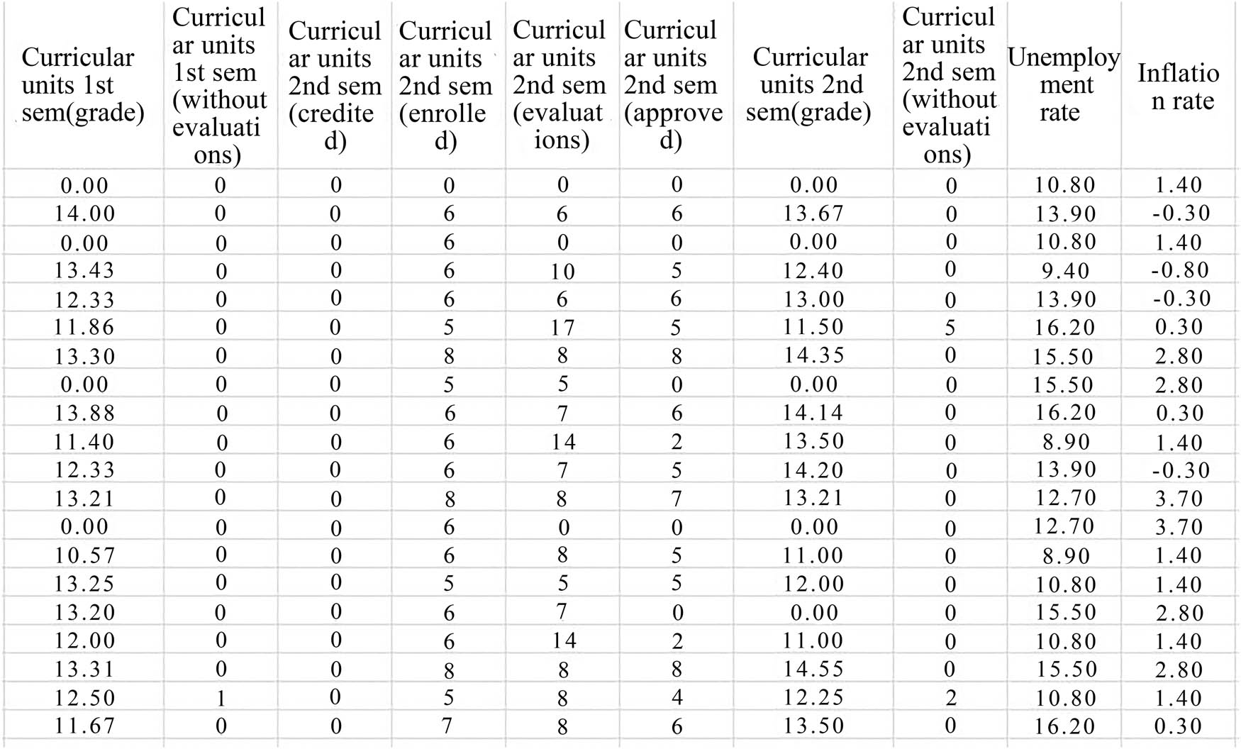
Partial data display after normalization encoding of student performance data.
2.2.2 Feature selection
For the teaching quality evaluation dataset, there are 28 specific questions and five additional attributes. PCA [17,18] was used to select the proportion of six questions with higher contribution rates, which were Q1, Q2, Q3, Q4, Q5, and Q6. The specific proportion is shown in Figure 3(a) and Figure 3(b). In Figure 3(a), the main components were mainly concentrated in PC1 and PC2, corresponding to Q1 and Q2, with the largest proportion. Correspondingly, in Figure 3(b), it can be seen that the total of Q1 and Q2 reached 86.76%. To further balance various component factors, the top six components were now extracted, totaling 91.41%, which could represent the typical performance of most data.
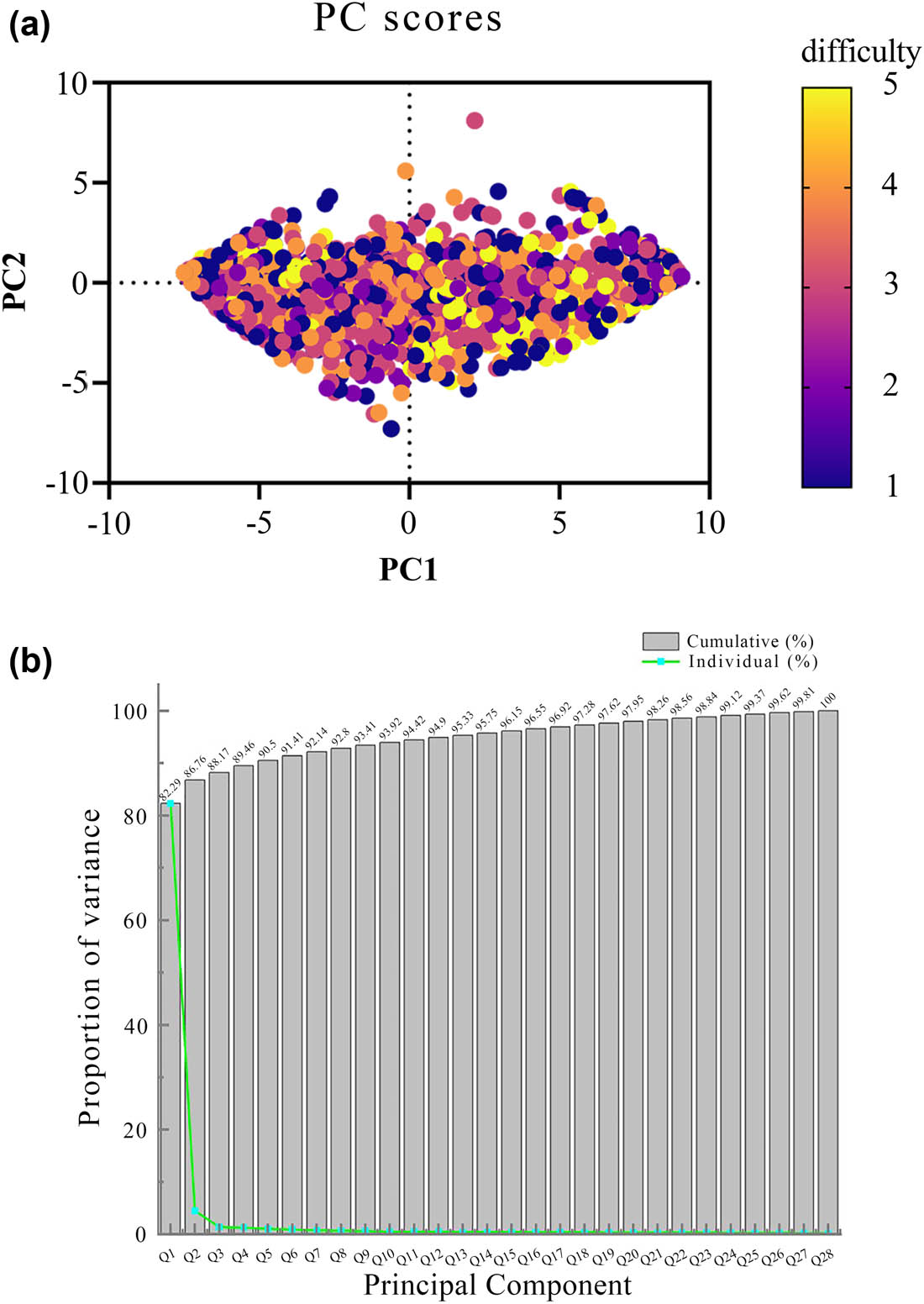
(a) Principal component analysis. (b) Principal component contribution rate.
3. ML algorithms
3.1 RF
RF [19,20] is a classifier composed of multiple DTs, each of which is independent of each other. The sample set N of the trained DT corresponds to the number of samples, and the test sample feature vector is X. The training program for a single DT mainly involves the following process: first, randomly sampling N times in N samples according to the bagging sampling rule as the root node training samples. The DT randomly selects m dimensions from the feature attribute M dimensions of nodes, where m is less than M. Next, their Gini impurity indices are calculated separately. The feature with the smallest index selected according to the minimum criterion is set as a node splitting attribute, and the splitting function is used to split the node into two subtrees until it reaches the leaf node.
The implementation steps of the RF classification process are as follows: the number of DTs n is determined as needed, and n training sets of the same size are obtained through random sampling. Second, by randomly rotating k attributes to obtain n attribute subsets in the attribute set, k = log2v, and using the DT algorithm to correspond the training set to the attribute subset, a DT is obtained. Finally, the DT is summarized and optimized to form an RF model. Based on the voting mechanism, the DT is selected to classify the predicted samples with the highest number of times, and the classification results are determined. The accuracy of the five models in evaluating student grades and teaching quality is shown in Figure 4. The RF model had an accuracy of 85.6% in evaluating student grades and 84.2% in evaluating teaching quality. In Figure 5, the RF model achieved an F1 score of 85.5% in the evaluation of student performance and 84.0% in the evaluation of teaching quality.
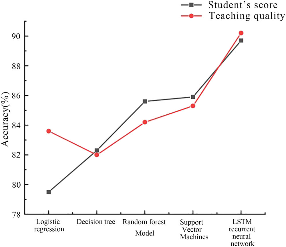
Estimated accuracy of the model in terms of student grades and student quality.
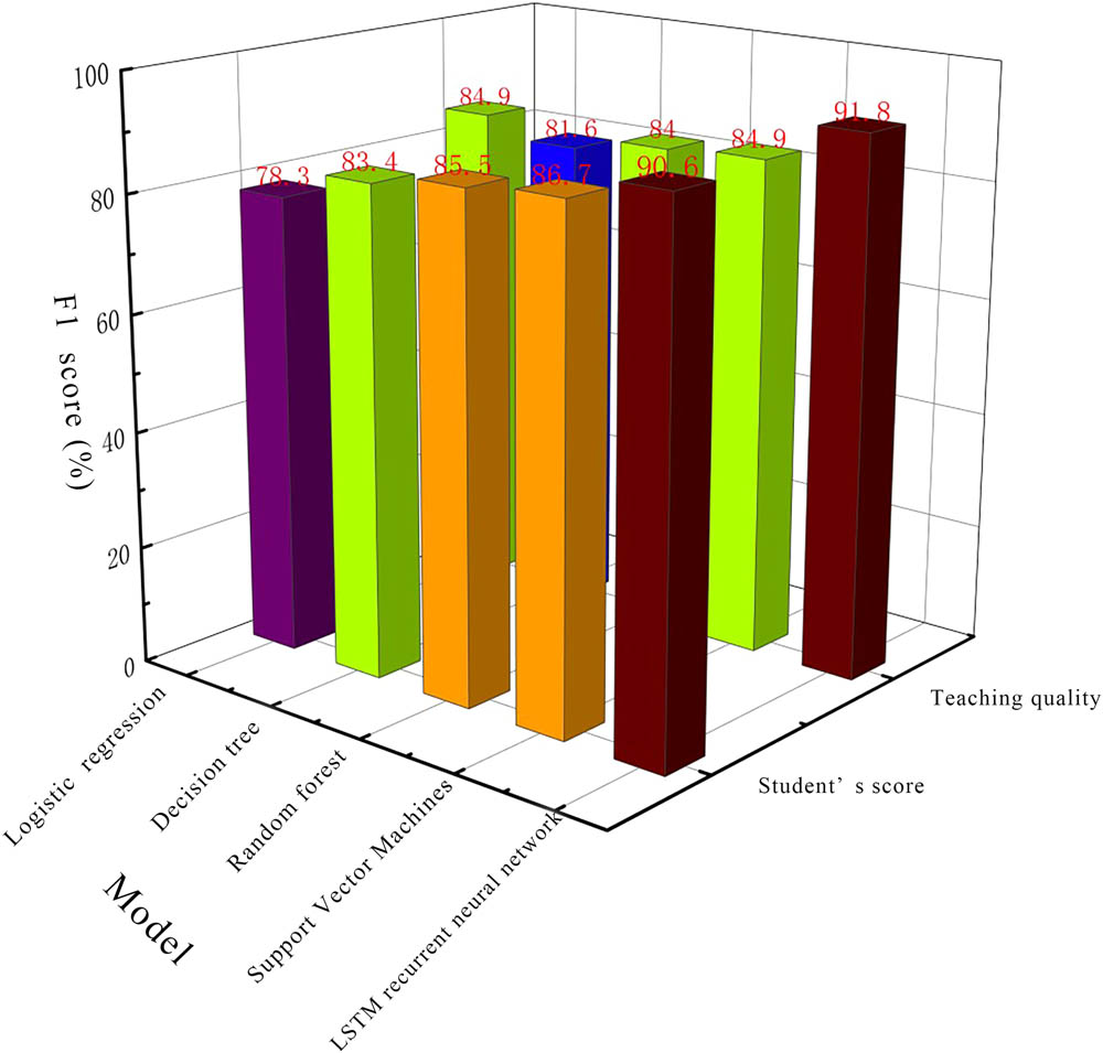
Estimated F1 score of the model in terms of student grades and student quality.
3.2 Decision tree
DT is a modeling method from tree roots, branches to branches. The DT algorithm [21] is a decision algorithm that adopts a tree structure, where each node corresponds to a judgment of an attribute; the branch corresponds to the judgment result, and the leaf corresponds to the final judgment result. The DT algorithm is a recursive process.
The training set is D, and the attribute set
3.3 SVM
SVM is an effective classification method based on statistical learning theory, which transforms the sample space into another feature space through nonlinear transformation and constructs a regression estimation function, where a suitable kernel function K(X i , Y i ) is defined for nonlinear transformation [22]. Given a training dataset on the feature space, the sample is set as x, and n is the vector; the calculation of m samples and output values is shown in formula (1).
x
i
For the case where the training set is linearly separable, the learning process of the SVM is a quadratic programming process, and the regression function calculation is shown in formula (2).
The SVM model had an accuracy of 85.9% in evaluating student grades and 85.3% in evaluating teaching quality. In Figure 5, the SVM model achieved an F1 score of 86.7% in the evaluation of student grades and 84.9% in the evaluation of teaching quality.
3.4 Logistic regression
Logistic regression is a supervised learning algorithm used to solve binary classification problems and can also be used for multi-classification problems. Its basic idea is to linearly combine input features and transform the linear output into probability values within the (0,1) interval through a special activation function. Logical regression is suitable for cases where label values are discrete, and its functional representation is shown in formula (3).
Among them,
The logistic regression classification model [23] uses a cost function to measure the precision of the model, and the regularized cost function is shown in formula (4).
Among them, the feature vector of the i-th data sample is represented as
The gradient descent algorithm [24] can be used to solve the parameter A vector. The minimization regularization cost function is upgraded, as shown in formulas (5) and (6).
Among them, j = 1,2,…n.
3.5 RNN
LSTM is a special recurrent network model that uses LSTM to capture time series information during the student learning process for predicting student grades. The model can fully consider the historical learning behavior of students to predict future trends in student performance. This helps to provide more accurate academic advice and intervention measures. LSTM is also used to analyze time series data during the teaching process, including the use of teaching resources, student participation, and teaching effectiveness. By modeling these sequence data, it can evaluate the quality of teaching and provide improvement suggestions to optimize the educational process. LSTM can also be used to analyze student learning behavior, including learning duration, learning activities, and the use of online learning platforms. It can provide a deeper understanding of student learning habits, thereby improving personalized teaching and providing personalized feedback.
LSTM is a special cyclic network model that uses special implicit units and is mainly used to process long time series data. This model mainly consists of forgetting threshold, input threshold, output threshold, and neural unit state. The forgetting threshold, as shown in formula (7), determines the information that needs to be discarded [25,26].
Among them,
The input threshold formula [27], as shown in formulas (8) and (9), can determine which new information is stored in the unit state.
Among them,
The unit state runs through the entire chain, and only small linear interactions make it easy to flow downward in a constant manner. The specific expression formula is shown in formula (10).
Among them,
The output threshold is the current value used to control how much unit state is output to the LSTM model, as shown in formulas (11) and (12).
Among them,
The LSTM model had an accuracy of 89.7% in evaluating student grades and 90.2% in evaluating teaching quality. In Figure 5, the LSTM model achieved an F1 score of 90.6% in student performance evaluation and 91.8% in teaching quality evaluation.
The specific process of the LSTM model is as follows: first, the output values of each neuron are calculated forward according to formulas (7)–(12), corresponding to five vector values, namely
3.6 Multi-classifier fusion
This study adopts a multi-classifier fusion strategy to fully leverage the advantages of different machine learning algorithms and improve the overall performance of the model. Different machine learning algorithms may exhibit different advantages in different data distributions and scenarios. In this article, by combining multiple algorithms, the robustness of the model can be improved, and it can perform well in all situations. Moreover, a single model may overfit a specific dataset, resulting in poor generalization ability for other data. Multi-classifier fusion can reduce the risk of overfitting and improve the generalization ability of models by integrating the opinions of multiple models. In addition, in practical applications, there may be a class imbalance in the data, and adopting a multi-classifier fusion strategy can better handle this imbalance. By adjusting the weight of each classifier, greater attention can be paid to its performance in minority categories, resulting in superior results in educational evaluation and rating scenarios.
4. Comparative experiments on multi-classifier models in scenarios of predicting student grades and teaching quality
4.1 Experimental environment
This experiment was based on a Windows 10 system and implemented using the TensorFlow framework in Python, using the Intel Core i7-6800k Central Processing Unit with 16GB of memory.
4.2 Model comparison experiment process in different scenarios
To verify the adaptability of the model, its performance was tested in different scenarios. The scenario was divided into two: student performance and teaching quality evaluation and grading. The model includes a single model, which is followed by logical regression, DT, RF, SVM, and LSTM RNN. The multiple classification models are sequentially combined into six types: logistic regression + DT, SVM + DT, LSTM RNN + RF, logistic regression + SVM, logistic regression + LSTM RNN, and DT + LSTM neural network. First, the data in the dataset were encoded and normalized, and feature selection was performed using PCA to evaluate the teaching quality of the data. Next, pre-normalized student performance data were used as input to a single model in sequence. In the pre-training phase of the entire experiment, all samples in the training set were first trained 30 times (epoch = 30). When adjusting the parameters, the number of training sessions was dynamically expanded to a multiple of 10 and stacked to 300 times (epoch = 300), and each training session took size = 50 data. By reducing the number of samples used in each iteration and taking size = 50 data for each training, the training process is accelerated and, to some extent, adapted to data diversity. The loss function and accuracy curve under the student performance scenario are shown in Figures 6–9. To prevent overfitting, in the logistic regression model, L1 regularization [29] was used to limit the weight size, reduce complexity, and avoid fitting phenomena. In the DT model, pruning techniques were used to delete some branches in the DT and reduce the depth of the tree. In the model of RF, the overfitting risk of a single model was reduced by combining multiple models through integrated methods. In the SVM model, different weights were assigned to each sample to balance the impact between different samples. This study has achieved the best results by setting the following parameters through multiple experiments. In the LSTM RNN model, this study set the dropout layer loss rate of the time network to 0.7 and the initial learning rate to 0.001. In addition, the weight attenuation coefficient for training was set to 0.0004 and the momentum was 0.9. Next, the effectiveness of a single model was tested on the validation set of student grades and teaching quality in sequence. Finally, six multi-classification models were trained and validated separately, and the performance of the model was verified by comparing parameters such as accuracy, precision, recall value, F1 score, and training duration in different scenarios.
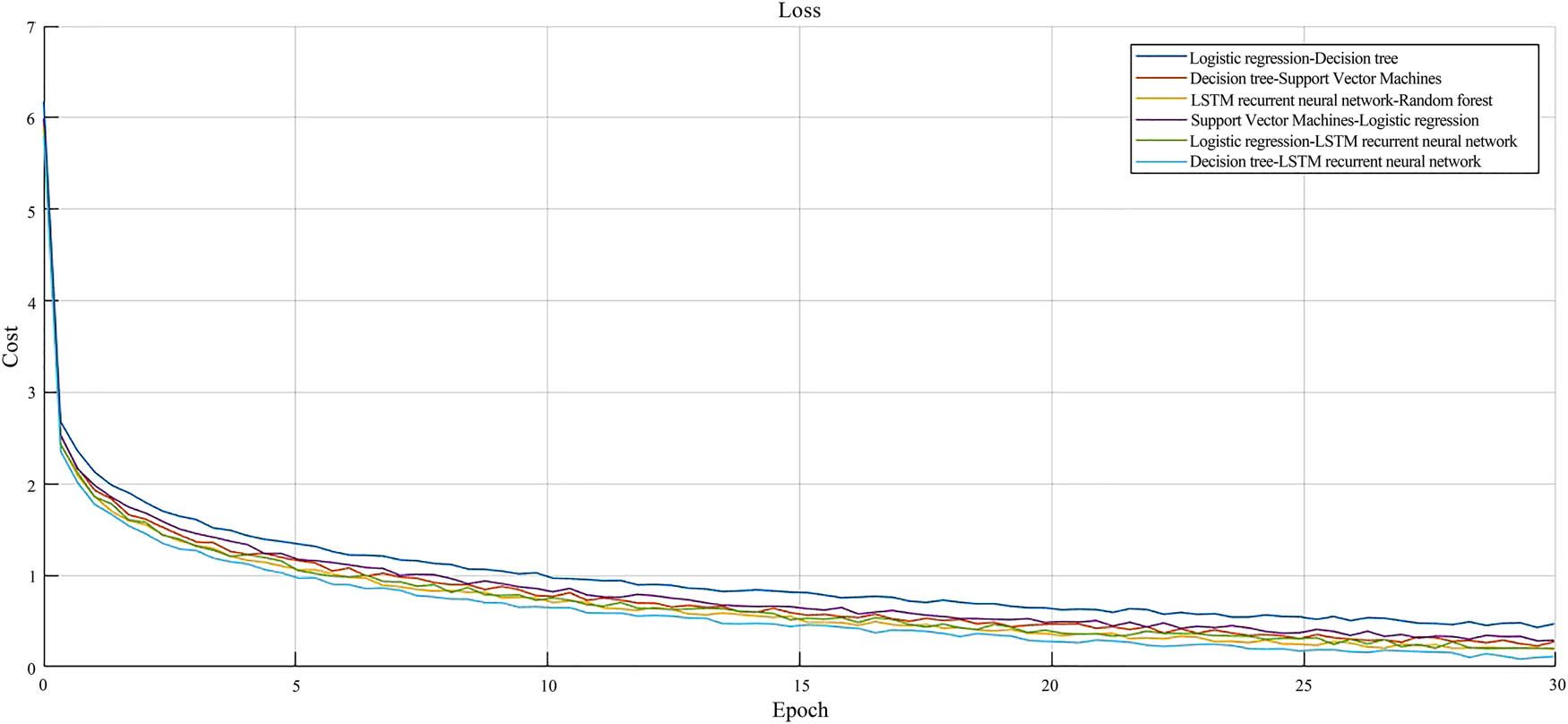
30 epochs loss function curve of the model.
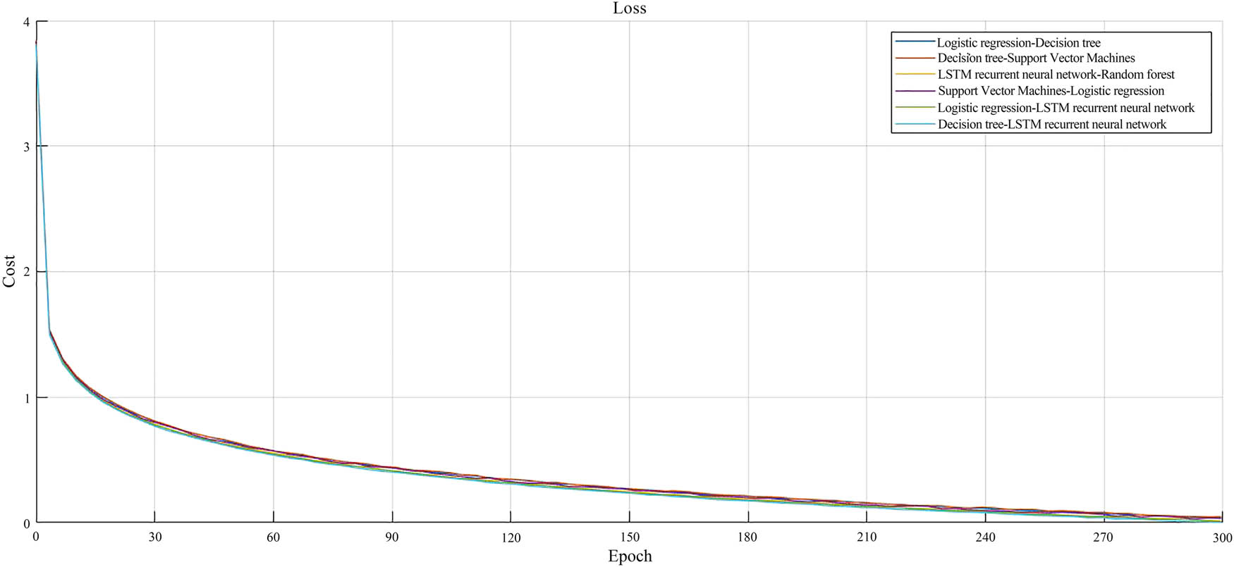
Model 300 epochs loss function curve.
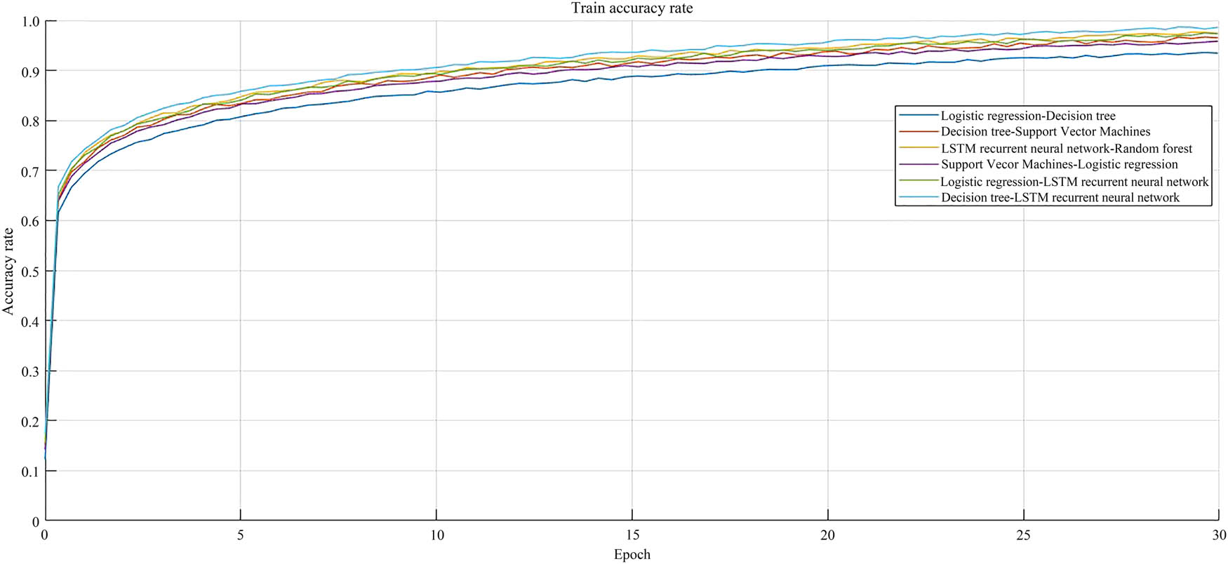
Accuracy curve of model 30 epochs.
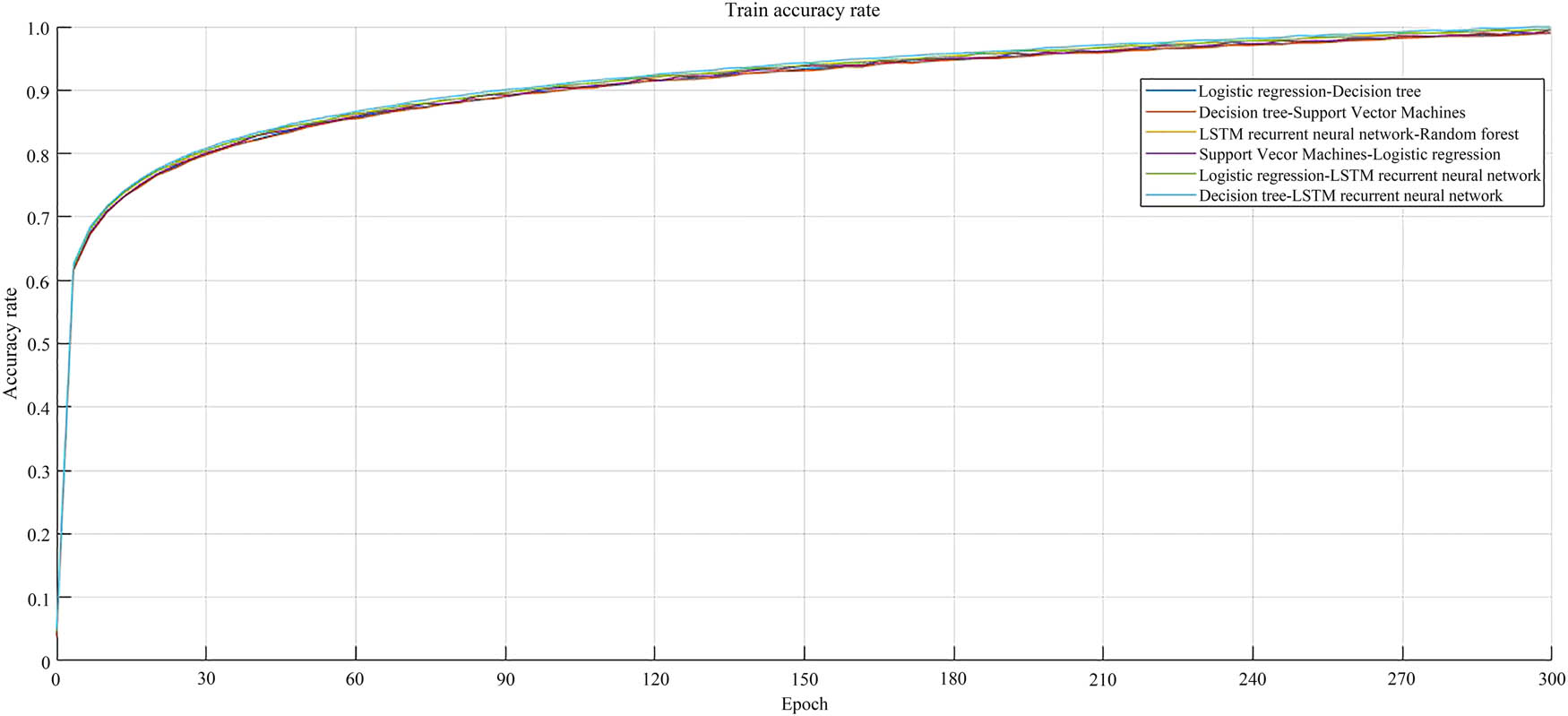
Accuracy curve of model 300 epochs.
In Figure 6, the horizontal axis represents the number of epochs, and the vertical axis represents the loss. Overall, after 30 epochs, the loss tended to range from 0 to 0.5, with the DT–LSTM RNN model having the smoothest loss function and the lowest loss; it was easier to converge, approaching 0.1, achieving ideal expectations. The loss of the LSTM RNN–RF model decreased from 6.0 to 0.3, with a decrease of 95% from the initial level, and the effect was quite impressive. The loss of the logistic regression–LSTM RNN model decreased from 6.0 to 0.4, a decrease of 5.6. The overall curve was similar to that of the LSTM RNN–RF model, but the LSTM RNN–RF model had less loss and better performance. In addition, the overall curves of the three curves were higher than the three combination models mentioned above, with a convergence range of 0.45–0.56. In summary, the LSTM RNN model had a better contribution to the combination model and had a good effect.
Figure 7 shows the loss function curve of the model for 300 epochs. Overall, after 300 epochs, the losses can converge between 0.01 and 0.05, with a maximum loss of only 3.8. Compared to the curve of 30 epochs, it can be analyzed that the minimum loss value decreased from 0.1 to 0.01, with a significant decrease, reaching the initial 90%. The DT–LSTM RNN model had the best performance, with a convergence value of 0.01 and the overall amplitude being the smoothest. The LSTM RNN–RF model had a slightly weaker performance, with a convergence value of 0.02. Compared to the curve with 30 epochs, the convergence value decreased by an initial 93%. For the logistic regression–LSTM RNN model, the curve was more jittery compared to the two combination models mentioned above, with a convergence value of 0.04. Compared to the DT–LSTM RNN model, the convergence value had increased by 0.03, resulting in poorer performance. In summary, the DT–LSTM RNN model and LSTM RNN–RF model showed good performance and were feasible for application in this experiment.
Figure 8 shows the accuracy curve of the model for 30 epochs. Overall, after 30 epochs, the evaluation accuracy of the six combined models reached 94.0–98.2%, with an average of 96.1%. In addition, the DT–LSTM RNN model was relatively flat and more stable overall. For the DT–LSTM RNN model, the estimation accuracy reached 98.2%, but it did not converge well. The LSTM RNN–RF model achieved an estimation accuracy of 97.1%, with a decrease of 1.2% compared to the DT–LSTM RNN model. The prediction accuracy of the logistic regression–LSTM RNN model reached 96.9%, which was closer to the curve of the LSTM RNN–RF model. However, the curve of the LSTM RNN–RF model was more stable, and the prediction accuracy of the logistic regression–LSTM RNN model was improved by 0.2%, resulting in better results. The other three models had lower estimation accuracy, ranging from 94.0 to 96.3%, and failed to converge well, resulting in worse results. In summary, the first two models had better performance and were more prone to convergence after multiple trainings.
In Figure 9, the horizontal axis represents 300 epochs, and the vertical axis represents the estimated accuracy. Overall, the overall curve was relatively stable with no significant differences, and the estimation accuracy tended to be between 99.2 and 9.9%. The prediction accuracy of the DT–LSTM RNN model reached 99.9%, and the curve was relatively stable, approaching convergence at 1.0. Compared with 30 epochs, the prediction accuracy improved by 1.7%, achieving the expected training effect. For the LSTM RNN–RF model, its estimation accuracy reached 99.8%, which was a significant decrease of 0.1% compared to the DT–LSTM RNN model. In addition, compared to 30 epochs, the estimation accuracy was improved by 2.7%, a significant improvement. The accuracy of logistic regression–LSTM RNN estimation reached 99.6%, which decreased by 0.3% compared to the DT–LSTM RNN model. However, both models converged well, and the results met the experimental requirements. In summary, the DT–LSTM RNN model and LSTM RNN–RF model had the best performance in predicting accuracy among the six combined models and could achieve good results in experiments.
5. Comparative experimental results and discussion of multi-classifier models in student performance and teaching quality
5.1 Evaluation criteria
When evaluating the results of the study, accuracy, precision, recall, and comprehensive evaluation index F1 score were used [30]. This article evaluated the evaluation and grading of student grades and teaching quality scenarios based on a multi-classification model.
Accuracy: it refers to the proportion of all correct judgments in the classification model to the total.
Precision: it refers to the proportion of truly correct predictions that are positive for all predictions.
Recall: it refers to the proportion of what is truly correct to what is actually positive.
F1 score: the f1 value is the arithmetic mean divided by the geometric mean, and the larger the result, the better the score. The f1 value is weighted for both precision and recall, and the f1 score belongs to 0–1. In this model, 1 represents the best recognition and classification results of the model, while 0 represents the worst.
In this study, multiple classifications were used as a whole. Taking teaching quality as an example, the actual positive class prediction is True Positive (TP), which means that 90 points of teaching quality are predicted as 90 points of teaching quality. The actual positive class prediction is False Negative (FN), which means that 90 points of teaching quality are predicted to be 60 points of teaching quality. The actual negative class is predicted to be False Positive (FP), which means that 60 points of teaching quality are predicted to be 90 points of teaching quality. The actual negative class prediction is True Negative (TN), which means that 60 points of teaching quality are predicted as 60 points of teaching quality.
5.2 Comparison of experimental results of multi-classifier models in student achievement and teaching quality scenarios
The evaluation results of LSTM RNN–RF in the scenario of student performance estimation and DT–LSTM RNN in the teaching quality evaluation are shown in Table 1.
Evaluation results of some students’ grades and teaching quality
| Student’s score | Teaching quality | ||||||
|---|---|---|---|---|---|---|---|
| Student number | Course number | Actual score | Prediction score | Teacher number | Class | Actual quality score | Prediction quality score |
| 50 | 9238 | 84.30 | 83.87 | 1 | 2 | 94.20 | 92.00 |
| 77 | 9254 | 72.92 | 69.70 | 1 | 10 | 97.10 | 98.40 |
| 96 | 9119 | 90.50 | 90.83 | 2 | 6 | 88.20 | 87.50 |
| 186 | 9147 | 65.46 | 68.60 | 3 | 5 | 93.70 | 92.40 |
| 280 | 9500 | 89.44 | 92.70 | 2 | 11 | 92.30 | 88.80 |
5.3 Comparative experimental discussion of multi-classifier models in student achievement and teaching quality scenarios
5.3.1 Error estimation and confusion matrix
From Table 1 analysis, it can be seen that the actual score of student 77 with course number 9254 was 72.92, located in the range of 70–80, but the predicted score was 69.70, located in the range of 60–70, which was one level lower than the estimated classification. According to the analysis of the student’s admission score and learning time, the admission score was not high and the learning time was short, so this model had errors in predicting student grades. The actual score of the student with course number 9,500 and course number 280 was 89.44, which belonged to the range of 80–90. However, the predicted score was 92.70, which belonged to the range of 90–100, and was one level higher overall. The reason for the opposite was the same. In the future, the prediction results will be more refined and integrated with various factors during training. For teaching quality, the teacher with teacher number 2 and class number 11 had an actual quality score of 92.30, which was between 90 and 100, but the predicted score was 88.80, which was between 80 and 90. The analysis of the data showed that the teacher’s teaching quality was very good, but the attendance was very low. Therefore, when analyzing the data, the model showed a slight decrease compared to the actual estimated results, and the overall effect was good.
For different score segment types, the LSTM RNN–RF model was used for predicting student performance scenarios, and the DT–LSTM RNN model was used for predicting teaching quality. The confusion matrix is shown in Figure 10. The horizontal axis represents the predicted type score segment, which is 0–60, 60–70, 70–80, 80–90, and 90–100 from left to right. The vertical axis represents the actual score segment, which is the same as the horizontal axis from top to bottom. For the confusion matrix of student performance estimation (left figure in Figure 10), the proportion of samples actually belonging to the corresponding actual category predicted to be the corresponding predicted category was highest in the 90–100 and 80–90 score ranges, and the proportion of correctly predicted samples reached 98%; the classification effect was very impressive, with a minimum concentration of 60–70, and the proportion of correctly predicted samples reaching 95%. In contrast, there were more classification errors, with 1% being incorrectly predicted as 0–60, 3% being incorrectly predicted as 70–80, and 1% being predicted as 80–90. The 70–80 score range was difficult to classify, only 96%, with 1% predicted as 80–90 and 3% predicted as 60–70. Other categories had good classification results and could meet practical application needs.
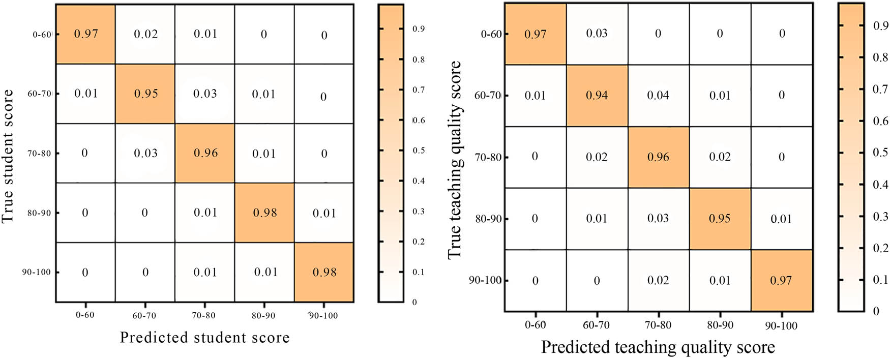
Confusion matrix between student performance and teaching quality estimation.
For the confusion matrix of teaching quality evaluation (shown in the right figure of Figure 10), the proportion of samples actually belonging to the corresponding actual category being predicted as the corresponding predicted category was highest in the 0–60 and 90–100 score ranges, and the proportion of correctly predicted samples reached 97%; the classification achieved ideal results, with a minimum concentration of 60–70, and the proportion of correctly predicted samples reached 94%. In contrast, there were more classification errors, with 1% being incorrectly predicted as 0–60, 4% being incorrectly predicted as 70–80, and 1% being predicted as 80–90. The 80–90 score range was difficult to classify, with only 95% predicted, with 1% predicted as 60–70, 3% predicted as 70–80, and 1% predicted as 90–100. Other categories were relatively low but had also achieved good practical results.
5.3.2 Comparison of the accuracy of different models in different scenarios
The comparison of estimation accuracy for different models in different scenarios is shown in Figure 11. In the scenario of predicting student grades, the logistic regression–DT model had the worst prediction performance, only 91.2%. The LSTM RNN–RF model achieved the best estimation performance, with an accuracy of 98.5%, which was 7.3% higher than logistic regression–DT. The logistic regression–LSTM RNN model achieved 97.3% improvement, which was 6.1% higher than the logistic regression–DT model, and the estimation accuracy was significantly improved. The DT–LSTM RNN model achieved 96.9% improvement, which was 5.7% higher than logistic regression–DT.
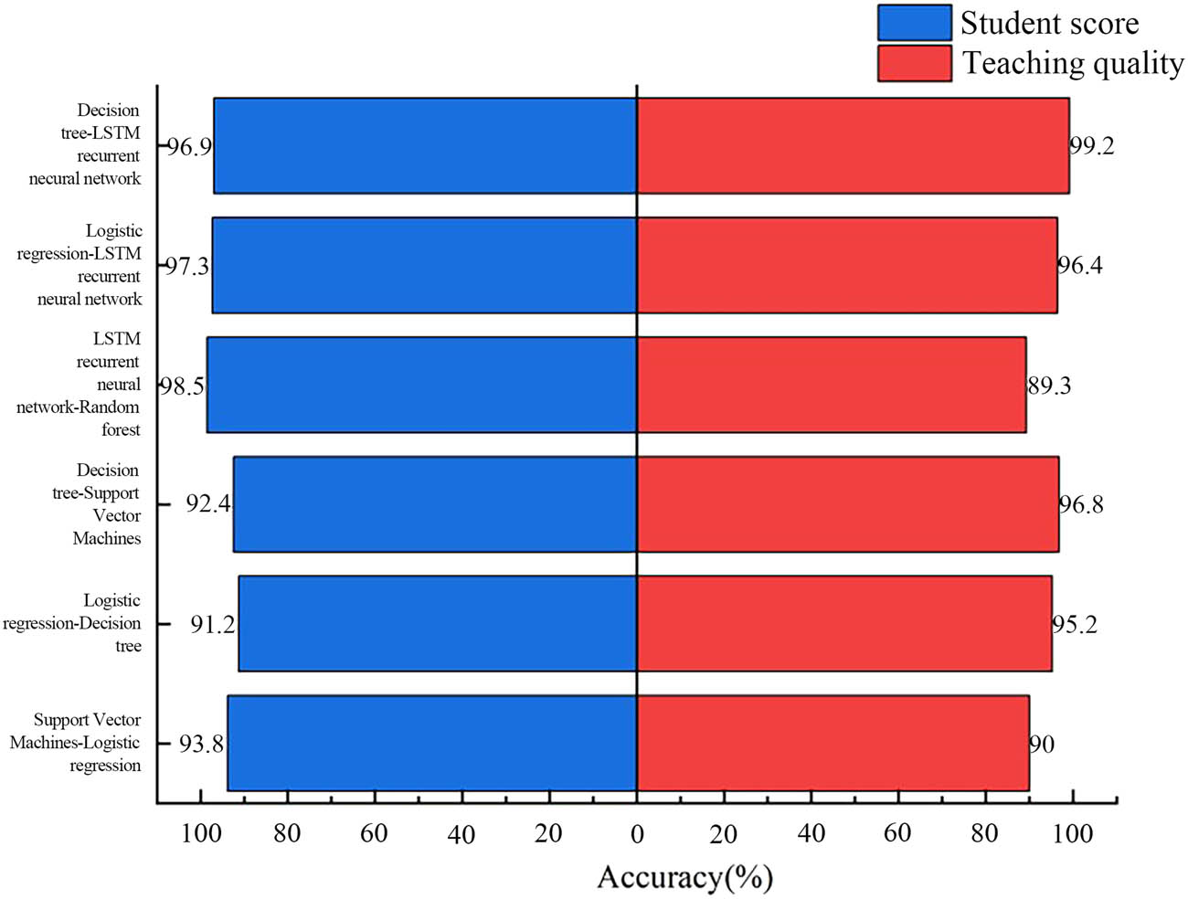
Comparison of the accuracy of different models in different scenarios.
In the scenario of predicting teaching quality, the DT–LSTM RNN model had the best prediction performance, reaching 99.2%, while the LSTM RNN–RF model had the worst prediction performance, only 89.3%. Compared with the estimation effect under the scenario of predicting student grades, the LSTM RNN–RF model achieved the best effect under the scenario of predicting student grades, but the effect on predicting teaching quality was not ideal. The effect of DT–LSTM RNN on student performance prediction was not the best, which showed that the same model had different adaptability to different scenarios. Analysis showed that DT–LSTM RNN is more suitable for evaluating teaching quality, precisely because DT is more suitable for interpretability and rule extraction of teaching quality. At the same time, LSTM RNN can capture long-term time dependencies and is suitable for analyzing changes in teaching quality over time. The LSTM RNN–RF model is more suitable for evaluating students’ grades, precisely because using LSTM RNN to capture students’ time series information, such as historical exam scores or learning behaviors, is more convenient and applicable. RF can be used to process other non-time series features, such as students’ background information and attendance rate, with stronger practicality.
5.3.3 Comparison of precision, recall, and F1 score in student performance evaluation and grading scenarios
The comparison of prediction, recall, and F1 score of different models under student grades is shown in Figure 12. The horizontal axis represents the classification of the model, and the vertical axis represents the proportion of parameters. Overall, the LSTM RNN–RF histogram had the highest precision of 97.4%, recall of 94.4%, and F1 score of 98.1%, achieving the best performance. Compared to the DT–LSTM RNN model, the distribution of the above three parameters increased by 1.8, 0.9, and 2.2%. The logistic regression–LSTM RNN histogram was second, with a precision of 96.2%, recall of 93.9%, and F1 score of 96.5%. Compared to the DT–LSTM RNN model, it increased by 0.6, 0.4, and 0.6%, respectively. In summary, analyzing the above parameters showed that the LSTM RNN–RF model achieved the best performance and stronger adaptability in student performance scenarios (Figure 13).
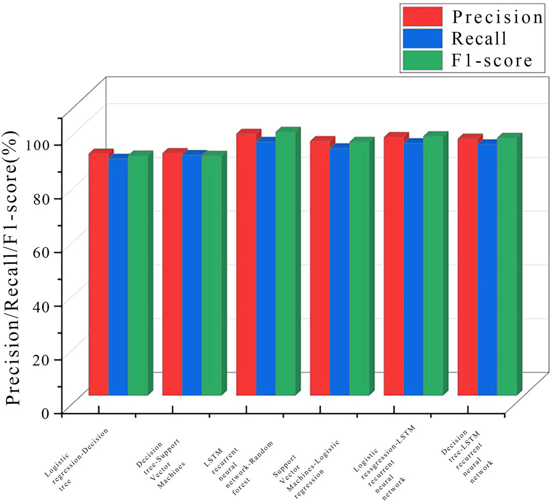
Comparison of precision, recall, and F1 score in student performance scenarios.
Comparison of precision, recall, and F1 score in teaching quality scenarios.
5.3.4 Comparison of precision, recall, and F1 score in the context of teaching quality evaluation and grading
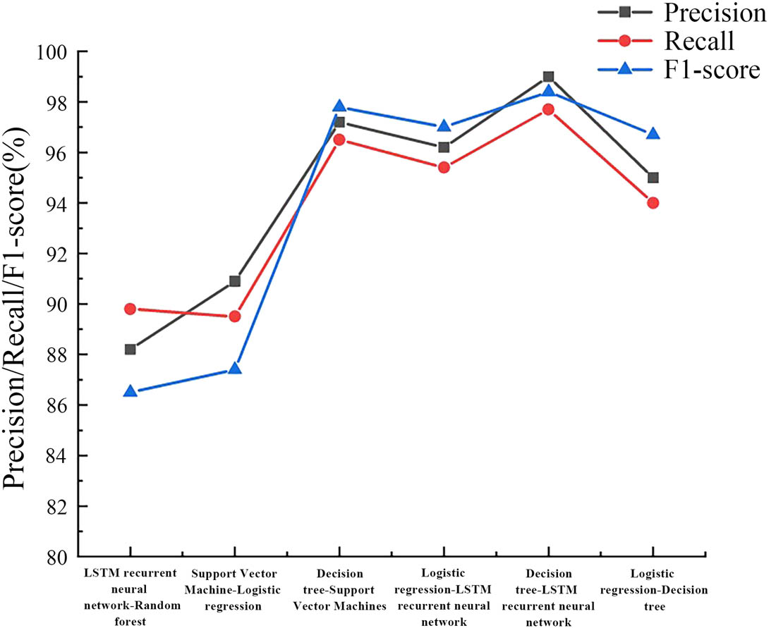
A comparison was made on the precision, recall, and F1 score of teaching quality estimation scenarios, as shown in Line chart 13. The red line represents the recall curve; the blue line represents the F1 score curve; and the gray line represents the precision curve. Overall, under the parameters of precision, the DT–LSTM RNN model had the highest prediction, reaching 99.0%, which was quite impressive. The DT–SVMs achieved good results in evaluating teaching quality, with a prediction of 97.2%, which was only 1.8% lower than the DT–LSTM RNN model. The LSTM RNN–RF model had the worst prediction performance, with a precision of only 88.2%, a recall of only 89.8%, and an F1 score of 86.5. Compared with the DT–LSTM RNN model, its prediction performance decreased by 10.8, 7.9, and 11.9% year-on-year, respectively. Compared to the scenario of predicting student performance, the LSTM RNN–RF model showed a 9.2% decrease in precision, while the DT–LSTM RNN model showed a 3.4% improvement in precision. In summary, the DT–LSTM RNN model was more applicable in the context of teaching quality estimation.
5.3.5 Comparison of training time for different models in different scenarios
For the training duration, this experiment compared and analyzed the training duration of six models in different scenarios, as shown in Table 2. In the scenario of estimating student grades, the training duration of logistic regression–DT was the shortest, only 2.3 h. The DT–SVMs model took second place and only took 3.5 h. The above two models are not complex and train quickly, but their accuracy in estimation is not as good. Although the LSTM RNN–RF model became larger after the introduction of LSTM, with a training time of 8.2 h, it achieved the best prediction accuracy by reducing the training time by 0.7 h compared to DT–LSTM RNN, indicating that the model has better adaptability to student grades and can be better understood by the model. In the scenario of estimating teaching quality, the training duration of logistic regression–DT was the shortest, only 1.8 h. The model with the best prediction accuracy, DT–LSTM RNN, reached 7.0 h, with a significant difference. However, compared to the LSTM RNN–RF model, it decreased by 0.5 h, and compared to the logistic regression–LSTM RNN model, it decreased by 0.8 h. It can be seen that in the scenario of student performance estimation, LSTM RNN–RF achieved good overall results, and in the scenario of teaching quality estimation, DT–LSTM RNN met practical needs comprehensively.
Comparison of training duration of different models in different scenarios
| Model (training time, h) | Logistic regression–DT | DT–SVMs | LSTM RNN–RF | SVMs–logistic regression | Logistic regression–LSTM RNN | DT–LSTM RNN |
|---|---|---|---|---|---|---|
| Student’s score | 2.3 | 3.5 | 8.2 | 4.9 | 8.4 | 8.9 |
| Teaching quality | 1.8 | 3.1 | 7.5 | 3.7 | 7.8 | 7.0 |
6. Conclusions
By using a multi-classification fusion strategy and fully considering the adaptability of the algorithm, this article studied the evaluation and grading of students in two scenarios with different grades and teaching quality. Finally, the experimental data of six fused multi-classification models, LSTM RNN–RF, SVMs–logistic regression, DT–SVMs, logistic regression–LSTM RNN, DT–LSTM RNN, and logistic regression–DT, were compared in the scenarios of student performance estimation and teaching quality estimation, and the experimental effects of educational evaluation and grading under different models were analyzed. The experimental results showed that the LSTM RNN–RF model had the strongest adaptability and higher prediction accuracy in the scenario of student performance estimation and was superior to a single RF model. In teaching quality scenarios, the DT–LSTM RNN model had the strongest adaptability and higher estimation accuracy and was superior to a single DT model. This experiment fully considered the adaptability of different ML algorithms to different scenarios to improve the prediction and classification accuracy of the model, which has stronger practicality. However, there are some shortcomings in this article’s experiment, such as a relatively large number of parameters and insufficient educational data scenarios. In the future, experiments would be conducted to further optimize the educational data scenarios by enriching them and reducing their weight.
-
Funding information: This study did not receive any funding in any form.
-
Author contributions: Xiangfen Ma contributed significantly by drafting the manuscript, conceptualizing the research framework, constructing the model, conducting data analysis, refining the language, and managing the image processing. All authors have read and agreed to the published version of the manuscript.
-
Conflict of interest: The author(s) declare(s) that there is no conflict of interest regarding the publication of this article.
-
Data availability statement: The data used to support the findings of this study are available from the corresponding author upon request.
References
[1] Hussain S, Khan MQ. Student-performulator: Predicting students’ academic performance at secondary and intermediate level using machine learning. Ann data Sci. 2023;10(3):637–55.10.1007/s40745-021-00341-0Search in Google Scholar PubMed PubMed Central
[2] Musso MF, Hernandez CFR, Cascallar EC. Predicting key educational outcomes in academic trajectories: a machine-learning approach. High Educ. 2020;80(5):875–94.10.1007/s10734-020-00520-7Search in Google Scholar
[3] Yun G, Ravi RV, Jumani AK. Analysis of the teaching quality on deep learning-based innovative ideological political education platform. Prog Artif Intell. 2023;12(2):175–86.10.1007/s13748-021-00272-0Search in Google Scholar
[4] Imran M, Latif S, Mehmood D, Muhammad S. Student academic performance prediction using supervised learning techniques. Int J Emerging Technol Learn. 2019;14(14):92–104.10.3991/ijet.v14i14.10310Search in Google Scholar
[5] Onan A. Mining opinions from instructor evaluation reviews: a deep learning approach. Comput Appl Eng Educ. 2020;28(1):117–38.10.1002/cae.22179Search in Google Scholar
[6] Ahmed N, Nandi D, Zaman AGM. Analyzing student evaluations of teaching in a completely online environment. Int J Mod Educ Comput Sci. 2022;14(6):13–24.10.5815/ijmecs.2022.06.02Search in Google Scholar
[7] Lu W, Vivekananda GN, Shanthini A. Supervision system of English online teaching based on machine learning. Prog Artif Intell. 2023;12(2):187–98.10.1007/s13748-021-00274-ySearch in Google Scholar
[8] Pan Y, Zhang L, Wu X, Mirosław JS. Multi-classifier information fusion in risk analysis. Inf Fusion. 2020;60(4):121–36.10.1016/j.inffus.2020.02.003Search in Google Scholar
[9] Zhang W, He H, Zhang S. A novel multi-stage hybrid model with Enhanced Multi-Population Niche Genetic Algorithm: an application in credit scoring. Expert Syst Appl. 2019;121(1):221–32.10.1016/j.eswa.2018.12.020Search in Google Scholar
[10] Pes B. Ensemble feature selection for high-dimensional data: a stability analysis across multiple domains. Neural Comput Appl. 2020;32(10):5951–73.10.1007/s00521-019-04082-3Search in Google Scholar
[11] Zhao H, Liu H. Multiple classifiers fusion and CNN feature extraction for handwritten digits recognition. Granul Comput. 2020;5(3):411–8.10.1007/s41066-019-00158-6Search in Google Scholar
[12] Khan UA, Javed A, Ashraf R. An effective hybrid framework for content based image retrieval (CBIR). Multimed Tools Appl. 2021;80(17):26911–37.10.1007/s11042-021-10530-xSearch in Google Scholar
[13] Su H, Yu Y, Du Q, Peijun D. Ensemble learning for hyperspectral image classification using tangent collaborative representation. IEEE Trans Geosci Remote Sens. 2020;58(6):3778–90.10.1109/TGRS.2019.2957135Search in Google Scholar
[14] AdrianChin YK, JosephNg PS, Eaw HC, Loh YF, Shibghatullah AS. JomDataMining: academic performance and learning behaviour dubious relationship. Int J Bus Inf Syst. 2022;41(4):548–68.10.1504/IJBIS.2022.127555Search in Google Scholar
[15] Berndt AE. Sampling methods. J Hum Lactation. 2020;36(2):224–6.10.1177/0890334420906850Search in Google Scholar PubMed
[16] Ahmad T, Aziz MN. Data preprocessing and feature selection for machine learning intrusion detection systems. ICIC Express Lett. 2019;13(2):93–101.Search in Google Scholar
[17] Huang D, Jiang F, Li K, Guoshi T, Guofu Z. Scaled PCA: a new approach to dimension reduction. Manag Sci. 2022;68(3):1678–95.10.1287/mnsc.2021.4020Search in Google Scholar
[18] Zebari R, Abdulazeez A, Zeebaree D, Dilovan AZ, Jwan NS. A comprehensive review of dimensionality reduction techniques for feature selection and feature extraction. J Appl Sci Technol Trends. 2020;1(2):56–70.10.38094/jastt1224Search in Google Scholar
[19] Boateng EY, Otoo J, Abaye DA. Basic tenets of classification algorithms K-nearest-neighbor, support vector machine, random forest and neural network: a review. J Data Anal Inf Process. 2020;8(4):341–57.10.4236/jdaip.2020.84020Search in Google Scholar
[20] Punia S, Nikolopoulos K, Singh SP, Jitendra KM, Konstantia L. Deep learning with long short-term memory networks and random forests for demand forecasting in multi-channel retail. Int J Prod Res. 2020;58(16):4964–79.10.1080/00207543.2020.1735666Search in Google Scholar
[21] Charbuty B, Abdulazeez A. Classification based on decision tree algorithm for machine learning. J Appl Sci Technol Trends. 2021;2(01):20–8.10.38094/jastt20165Search in Google Scholar
[22] Styawati S, Mustofa K. A support vector machine-firefly algorithm for movie opinion data classification. IJCCS. 2019;13(3):219–30.10.22146/ijccs.41302Search in Google Scholar
[23] Cabero‐Almenara J, Guillen‐Gamez FD, Ruiz‐Palmero J, Palacios-Rodriguez A. Teachers’ digital competence to assist students with functional diversity: identification of factors through logistic regression methods. Br J Educ Technol. 2022;53(1):41–57.10.1111/bjet.13151Search in Google Scholar
[24] Reisizadeh A, Mokhtari A, Hassani H, Ramtin P. An exact quantized decentralized gradient descent algorithm. IEEE Trans Signal Process. 2019;67(19):4934–47.10.1109/TSP.2019.2932876Search in Google Scholar
[25] Yu Y, Si X, Hu C, Zhang J. A review of recurrent neural networks: LSTM cells and network architectures. Neural Comput. 2019;31(7):1235–70.10.1162/neco_a_01199Search in Google Scholar PubMed
[26] Chen F, Cui Y. Utilizing student time series behaviour in learning management systems for early prediction of course performance. J Learn Anal. 2020;7(2):1–17.10.18608/jla.2020.72.1Search in Google Scholar
[27] Wei X. Learning performance prediction based on artificial intelligence LSTM recurrent neural network. ChJ ICT Educ. 2022-28;04:123–8.Search in Google Scholar
[28] Liu Q, Huang Z, Yin Y, Enhong C, Hui X, Yu S. Ekt: Exercise-aware knowledge tracing for student performance prediction. IEEE Trans Knowl Data Eng. 2019;33(1):100–15.10.1109/TKDE.2019.2924374Search in Google Scholar
[29] Skourt BA, El Hassani A, Majda A. Mixed-pooling-dropout for convolutional neural network regularization. J King Saud Univ-Comput Inf Sci. 2022;34(8):4756–62.10.1016/j.jksuci.2021.05.001Search in Google Scholar
[30] Lee CA, Tzeng JW, Huang NF, Yu SS. Prediction of student performance in massive open online courses using deep learning system based on learning behaviors. Educ Technol Soc. 2021;24(3):130–46.Search in Google Scholar
© 2024 the author(s), published by De Gruyter
This work is licensed under the Creative Commons Attribution 4.0 International License.
Articles in the same Issue
- Research Articles
- A study on intelligent translation of English sentences by a semantic feature extractor
- Detecting surface defects of heritage buildings based on deep learning
- Combining bag of visual words-based features with CNN in image classification
- Online addiction analysis and identification of students by applying gd-LSTM algorithm to educational behaviour data
- Improving multilayer perceptron neural network using two enhanced moth-flame optimizers to forecast iron ore prices
- Sentiment analysis model for cryptocurrency tweets using different deep learning techniques
- Periodic analysis of scenic spot passenger flow based on combination neural network prediction model
- Analysis of short-term wind speed variation, trends and prediction: A case study of Tamil Nadu, India
- Cloud computing-based framework for heart disease classification using quantum machine learning approach
- Research on teaching quality evaluation of higher vocational architecture majors based on enterprise platform with spherical fuzzy MAGDM
- Detection of sickle cell disease using deep neural networks and explainable artificial intelligence
- Interval-valued T-spherical fuzzy extended power aggregation operators and their application in multi-criteria decision-making
- Characterization of neighborhood operators based on neighborhood relationships
- Real-time pose estimation and motion tracking for motion performance using deep learning models
- QoS prediction using EMD-BiLSTM for II-IoT-secure communication systems
- A novel framework for single-valued neutrosophic MADM and applications to English-blended teaching quality evaluation
- An intelligent error correction model for English grammar with hybrid attention mechanism and RNN algorithm
- Prediction mechanism of depression tendency among college students under computer intelligent systems
- Research on grammatical error correction algorithm in English translation via deep learning
- Microblog sentiment analysis method using BTCBMA model in Spark big data environment
- Application and research of English composition tangent model based on unsupervised semantic space
- 1D-CNN: Classification of normal delivery and cesarean section types using cardiotocography time-series signals
- Real-time segmentation of short videos under VR technology in dynamic scenes
- Application of emotion recognition technology in psychological counseling for college students
- Classical music recommendation algorithm on art market audience expansion under deep learning
- A robust segmentation method combined with classification algorithms for field-based diagnosis of maize plant phytosanitary state
- Integration effect of artificial intelligence and traditional animation creation technology
- Artificial intelligence-driven education evaluation and scoring: Comparative exploration of machine learning algorithms
- Intelligent multiple-attributes decision support for classroom teaching quality evaluation in dance aesthetic education based on the GRA and information entropy
- A study on the application of multidimensional feature fusion attention mechanism based on sight detection and emotion recognition in online teaching
- Blockchain-enabled intelligent toll management system
- A multi-weapon detection using ensembled learning
- Deep and hand-crafted features based on Weierstrass elliptic function for MRI brain tumor classification
- Design of geometric flower pattern for clothing based on deep learning and interactive genetic algorithm
- Mathematical media art protection and paper-cut animation design under blockchain technology
- Deep reinforcement learning enhances artistic creativity: The case study of program art students integrating computer deep learning
- Transition from machine intelligence to knowledge intelligence: A multi-agent simulation approach to technology transfer
- Research on the TF–IDF algorithm combined with semantics for automatic extraction of keywords from network news texts
- Enhanced Jaya optimization for improving multilayer perceptron neural network in urban air quality prediction
- Design of visual symbol-aided system based on wireless network sensor and embedded system
- Construction of a mental health risk model for college students with long and short-term memory networks and early warning indicators
- Personalized resource recommendation method of student online learning platform based on LSTM and collaborative filtering
- Employment management system for universities based on improved decision tree
- English grammar intelligent error correction technology based on the n-gram language model
- Speech recognition and intelligent translation under multimodal human–computer interaction system
- Enhancing data security using Laplacian of Gaussian and Chacha20 encryption algorithm
- Construction of GCNN-based intelligent recommendation model for answering teachers in online learning system
- Neural network big data fusion in remote sensing image processing technology
- Research on the construction and reform path of online and offline mixed English teaching model in the internet era
- Real-time semantic segmentation based on BiSeNetV2 for wild road
- Online English writing teaching method that enhances teacher–student interaction
- Construction of a painting image classification model based on AI stroke feature extraction
- Big data analysis technology in regional economic market planning and enterprise market value prediction
- Location strategy for logistics distribution centers utilizing improved whale optimization algorithm
- Research on agricultural environmental monitoring Internet of Things based on edge computing and deep learning
- The application of curriculum recommendation algorithm in the driving mechanism of industry–teaching integration in colleges and universities under the background of education reform
- Application of online teaching-based classroom behavior capture and analysis system in student management
- Evaluation of online teaching quality in colleges and universities based on digital monitoring technology
- Face detection method based on improved YOLO-v4 network and attention mechanism
- Study on the current situation and influencing factors of corn import trade in China – based on the trade gravity model
- Research on business English grammar detection system based on LSTM model
- Multi-source auxiliary information tourist attraction and route recommendation algorithm based on graph attention network
- Multi-attribute perceptual fuzzy information decision-making technology in investment risk assessment of green finance Projects
- Research on image compression technology based on improved SPIHT compression algorithm for power grid data
- Optimal design of linear and nonlinear PID controllers for speed control of an electric vehicle
- Traditional landscape painting and art image restoration methods based on structural information guidance
- Traceability and analysis method for measurement laboratory testing data based on intelligent Internet of Things and deep belief network
- A speech-based convolutional neural network for human body posture classification
- The role of the O2O blended teaching model in improving the teaching effectiveness of physical education classes
- Genetic algorithm-assisted fuzzy clustering framework to solve resource-constrained project problems
- Behavior recognition algorithm based on a dual-stream residual convolutional neural network
- Ensemble learning and deep learning-based defect detection in power generation plants
- Optimal design of neural network-based fuzzy predictive control model for recommending educational resources in the context of information technology
- An artificial intelligence-enabled consumables tracking system for medical laboratories
- Utilization of deep learning in ideological and political education
- Detection of abnormal tourist behavior in scenic spots based on optimized Gaussian model for background modeling
- RGB-to-hyperspectral conversion for accessible melanoma detection: A CNN-based approach
- Optimization of the road bump and pothole detection technology using convolutional neural network
- Comparative analysis of impact of classification algorithms on security and performance bug reports
- Cross-dataset micro-expression identification based on facial ROIs contribution quantification
- Demystifying multiple sclerosis diagnosis using interpretable and understandable artificial intelligence
- Unifying optimization forces: Harnessing the fine-structure constant in an electromagnetic-gravity optimization framework
- E-commerce big data processing based on an improved RBF model
- Analysis of youth sports physical health data based on cloud computing and gait awareness
- CCLCap-AE-AVSS: Cycle consistency loss based capsule autoencoders for audio–visual speech synthesis
- An efficient node selection algorithm in the context of IoT-based vehicular ad hoc network for emergency service
- Computer aided diagnoses for detecting the severity of Keratoconus
- Improved rapidly exploring random tree using salp swarm algorithm
- Network security framework for Internet of medical things applications: A survey
- Predicting DoS and DDoS attacks in network security scenarios using a hybrid deep learning model
- Enhancing 5G communication in business networks with an innovative secured narrowband IoT framework
- Quokka swarm optimization: A new nature-inspired metaheuristic optimization algorithm
- Digital forensics architecture for real-time automated evidence collection and centralization: Leveraging security lake and modern data architecture
- Image modeling algorithm for environment design based on augmented and virtual reality technologies
- Enhancing IoT device security: CNN-SVM hybrid approach for real-time detection of DoS and DDoS attacks
- High-resolution image processing and entity recognition algorithm based on artificial intelligence
- Review Articles
- Transformative insights: Image-based breast cancer detection and severity assessment through advanced AI techniques
- Network and cybersecurity applications of defense in adversarial attacks: A state-of-the-art using machine learning and deep learning methods
- Applications of integrating artificial intelligence and big data: A comprehensive analysis
- A systematic review of symbiotic organisms search algorithm for data clustering and predictive analysis
- Modelling Bitcoin networks in terms of anonymity and privacy in the metaverse application within Industry 5.0: Comprehensive taxonomy, unsolved issues and suggested solution
- Systematic literature review on intrusion detection systems: Research trends, algorithms, methods, datasets, and limitations