A modified Hoek–Brown model considering softening effects and its applications
-
Lei Zhang
 ,
Zhihua Tan
,
Zhihua Tan

Abstract
Considering that the traditional Hoek–Brown model only accounts for strain hardening effects in rock materials, while many rock materials exhibit strain softening effects under large deformation, a modified Hoek–Brown model has been developed to simultaneously describe both material hardening and softening characteristics. This enhancement builds upon the traditional Hoek–Brown model by introducing plastic internal variables that characterize material damage or degradation. To address numerical singularities and convergence difficulties encountered during the implementation of the modified Hoek–Brown model, a function smoothing method is employed. The physical significance of model parameters in the modified model is clarified through theoretical analysis and single-factor variable analysis methods. Finally, the modified Hoek–Brown model is applied to practical engineering calculations. The study results demonstrate that the modified Hoek–Brown model can effectively account for both strain hardening and strain softening effects in materials. The function smoothing method proves to be effective in mitigating numerical singularities and convergence issues encountered in the implementation of the modified Hoek–Brown model. For soft rock tunnels, when significant displacements occur in the surrounding rock, both displacements and stresses around the tunnel calculated using the modified Hoek–Brown model are more consistent with engineering reality than those obtained using the traditional Hoek–Brown model. It is recommended to consider applying the modified Hoek–Brown model in practical engineering calculations.
1 Introduction
In practical construction, such as during excavation of underground shafts, tunnels, and similar structures, the stress conditions of adjacent or nearby rock masses continue to change after excavation [1]. The stress field within the rock mass also undergoes continual alteration. Studying the mechanical properties and failure mechanisms of rock materials under stress is crucially significant. Strength criteria determine the stress and strain conditions under which rock specimens or rock engineering structures are likely to fail. Current failure theories can explain certain aspects of rock behavior well but often fail to generalize to complex stress conditions, particularly where many rock constitutive models cannot account for strain softening effects, posing significant challenges for engineering applications [2,3].
Many scholars have conducted extensive research on rock damage constitutive models from various perspectives and approaches based on various rock strength theories and failure theories to consider the strain softening effects of rocks. Currently, there are two main research methods for mechanical constitutive models of rock types: first, assuming that rocks follow certain mathematical or physical models, conducting loading and unloading tests to obtain experimental data, and then deriving the constitutive model of rocks; second, combining relevant theories of probability theory in mathematics, introducing the Weibull formula, and assuming that the micro unit destruction of rocks follows this formula, deducing the rock’s constitutive model. Gao et al. [4], based on statistical theory and damage mechanics, defined a rock fracture intensity variable from a mechanical perspective, where the work done by friction between fracture surfaces equals the strain energy released upon material fracture. They assumed that the strength distribution of rock micro-cubes follows a Weibull distribution and the stress levels satisfy the Hoek–Brown criterion. They derived a constitutive model for fractured rock masses and validated it using experimental data and discrete element methods. Wang et al. [5] developed a thermo-hydro-mechanical constitutive model based on an internal variable theory to simulate the damage and failure of rocks under freeze–thaw cycles. Zhang et al. [6] simplified cold-region rocks under geostress into three forms: complete failure, weak failure, and non-failure units. They represented the degree of unit damage by changing the elastic modulus and established a constitutive model for freeze-thawing rocks that considers softening effects. Yang et al. [7] summarized the stress–strain relationships of rocks under conventional triaxial compression test conditions, exploring the underlying mechanisms and improving classical plastic statistical damage models. They derived a constitutive model for rocks under conventional triaxial compression test conditions and preliminarily validated it using results from such tests. The results indicate that the modified constitutive model effectively and comprehensively reflects rock strain softening and expansion, capturing the transition from brittle flow to plastic flow characteristics with increasing confining pressure. Wei et al. [8] developed an elasto-plastic constitutive model that considers both fracture and plastic deformation for deep rock masses experiencing high stress conditions. Assuming that the strength of rock micro-elements follows a Weibull random distribution, Chen and Qiao [9], based on the Drucker–Prager criterion, energy principles, and fracture damage theory, derived a constitutive model that accounts for the effects of crack propagation length and joint closure friction in rock masses. The theoretical constitutive model curve of the model fits well with experimental constitutive curves of discontinuous jointed rock masses. A comparison between the effects considering and not considering the crack propagation length and joint friction effects showed superiority in the former case, validating the model’s rationality and effectiveness. Li et al. [10], through an analysis of rock damage mechanisms, identified correlations between damaged and undamaged specimens. Using the Mohr–Coulomb criterion as a basis, they established a constitutive model for rock materials considering damage under triaxial compression conditions and conducted simulation analysis validation. The results indicate that the established model effectively reflects the stress–strain relationship throughout the rock failure process. Xie et al. [11], based on modified Harris functions and analysis of indoor shear test results, proposed a new serrated rock constitutive model. Validation results demonstrate that the model accurately reflects the variation trend of peak shear curves, with straightforward parameter estimation and physically meaningful parameters. In order to elucidate the complete shear deformation evolution of rock materials, Xin et al. [12] established a macroscopic constitutive relationship for rock shear deformation by calculating micro-pore shear deformations and solid skeleton deformations. Validation results show that the established constitutive model can characterize the entire process of shear deformation and failure evolution in rocks, including stages such as compaction deformation, linear elastic deformation, shear hardening deformation, shear softening deformation, bimodal phenomena, and residual deformation stages. Within the framework of existing shear constitutive models, Xie et al. [13,14] assumed rock materials composed of relatively intact elements and damaged elements, establishing a rock constitutive model that considers softening effects. Based on the strain equivalence hypothesis and assuming the statistical distribution of micro-element strength follows a Weibull distribution, with micro-element failure governed by the Hoek–Brown criterion, Chen et al. [15] derived the relationship between rock micro-element strength and damage variables. They developed a new statistical damage constitutive model based on the Hoek–Brown criterion. Validation confirmed that the new model effectively describes the entire stress–strain relationship during the rock failure process. Bian et al. [16] estimated the mechanical properties of shale specimens over immersion time through laboratory tests. They subsequently investigated the degradation mechanisms of shale parameters under immersion conditions using X-ray diffraction and scanning electron microscopy at the microscopic level. They established a rock constitutive model considering the effects of pore compression under uniaxial loading conditions. Based on the assumption that the elastic modulus of rock microstructural units approximately follows a Weibull distribution and integrating strain energy density theory, Wen et al. [17] developed a damage constitutive model for rocks. A comparison of the simulation results from the new model with theoretical curves from existing models and experimental curves under uniaxial loading demonstrated that the new model effectively characterizes the stress–strain relationship of rocks. Based on the principles of statistical strength theory and damage mechanics and incorporating the Lemaitre strain equivalence hypothesis with consideration of acidic environments, Qu et al. [18] studied the freeze–thaw damage evolution mechanisms of sandstone specimens. They developed damage evolution equations and a constitutive model for rocks. Considering freeze–thaw and loading conditions, Fang et al. [19] utilized statistical methods to establish a damage constitutive model for rocks and validated its rationality. Based on triaxial compression creep tests under high confining pressure and high water pressure conditions for sandstone, Jiang et al. [20] concatenated a nonlinear viscoplastic model reflecting accelerated creep characteristics of rocks and a Burgers model. They constructed a new six-element nonlinear viscoelastic–plastic creep model and identified model parameters, verifying its correctness and rationality using experimental results. To more accurately quantify the mechanical properties of rocks after freeze–thaw cycles from a damage perspective, Lin et al. [21], based on the coupling damage hypothesis of rocks and utilizing the lognormal distribution commonly used in engineering reliability analysis and strain strength theory, established a statistical damage constitutive model for rocks under freeze–thaw cycles. Combining the Mohr–Coulomb criterion with energy dissipation theory and considering the hardening and softening characteristics of rocks during loading, Ma et al. [22] employed a non-associated plastic flow rule to describe the plastic deformation of rocks. They established a damage-plasticity constitutive model for rocks by dividing dissipated energy during the damage process by the rate of damage energy consumption. Meng et al. [23], through conventional triaxial compression tests, obtained stress–strain curves of red sandstone after freeze–thaw cycles. They then used logistic equations to reduce the ultimate stress and elastic modulus based on the number of freeze–thaw cycles. The study results indicated that with an increasing number of freeze–thaw cycles, the extent of rock damage intensified, leading to greater reductions in ultimate stress and elastic modulus, decreased compressive strength, enhanced plastic properties, and confining pressure mitigated rock damage.
In summary, numerous scholars have developed constitutive models that account for rock damage to address the softening effects of rocks. However, many of these models are quite complex, which directly limits their practical application in engineering. Considering that the Hoek–Brown strength criterion can be applied to rocks under various complex stress conditions and compared to several other classic strength criteria, it reflects the inherent nonlinear failure characteristics of rocks, including the effects of various factors such as minimum principal stress regions, low stress areas, and tensile stress regions on strength [24,25]. The Hoek–Brown criterion has become one of the most widely used and influential rock strength criteria to date [26,27,28,29], having a significant impact on engineering practice. Therefore, this article attempts to introduce internal variables based on the Hoek–Brown strength criterion to develop a modified Hoek–Brown model that accounts for rock softening effects.
2 Modified Hoek–Brown model considering softening effects
Building upon the traditional Hoek–Brown model, a modified version is proposed by introducing internal variables that characterize material degradation, thus enabling the description of material softening effects. This modified model is outlined as follows.
2.1 Elasticity relationship
where
2.2 Plastic potential function and yield function
The yield criterion of the traditional Hoek–Brown model is given by
where
Considering a specific rock material, the model parameters
Equation (2) can been considered as it comprises two terms,
Here, the internal variable D represents the degree of damage to the rock material as deformation progresses. Model parameters n and
The modified model employs a non-associated flow rule, where the plastic potential function used is similar to equation (3), with the difference that m in equation (3) is replaced by
2.3 Hardening rule
In the modified yield function in equation (3), which includes the plastic internal variable D, it is essential for a complete constitutive model to specify the evolution rule of D. Upon initial yielding of the rock material, the internal variable D, which characterizes rock damage, should be 0.0. As deformation of the rock progresses, the damage to the rock gradually intensifies, and D increases from 0.0 to 1.0, indicating that the rock material reaches residual strength. Considering that once damage occurs in the rock, its rate of damage development accelerates with continued deformation, an exponential function is employed to describe the evolution rule of the internal variable D.
where k represents the parameter governing the evolution rate of the internal variable D;
3 Numerical implementation of the modified model
Before conducting in-depth analysis and engineering applications of the modified model, it is essential to first implement it numerically. For the modified model, numerical implementation necessitates addressing the issues of three-dimensional formulation of the yield function and the presence of corner points in the principal stress space of the yield function.
3.1 Three-dimensional formulation of the yield function
Considering the satisfaction between principal stresses and stress invariants,
Substituting this equation into the yield function, equation (3), the following equation can be easily obtained:
where
where
3.2 Smoothing treatment of yield functions and plastic potential functions
By differentiating the plastic potential function with respect to stress
The stress rod angle
where
When the stress rod angle
where a is a parameter representing the degree of smoothness. Clearly, as a increases, the transition segment from
When the stress rod angle
where
When the stress rod angle
Combining the two smoothing transition equations, equations (12) and (15) yield the following smoothed yield function:
Clearly, the piecewise function corresponding to equation (16) satisfies continuity of zeroth and first-order derivatives, effectively avoiding numerical singularity issues during the numerical implementation process.
3.3 Numerical implementation of the model
The fundamental equations to be solved for the numerical implementation of the modified model using implicit algorithms are as follows:
where the physical quantities indexed with
4 Analysis of model parameters for the modified model
4.1 Physical meanings of model parameters
Before applying the modified model in engineering practice, it is essential to determine the model parameters. Clarifying the physical meanings of each model parameter is often necessary prior to their determination. As shown in Table 1, the model parameters of the modified model can be categorized into three classes. The first class includes parameters related to elasticity, such as elastic modulus E and Poisson’s ratio
Physical meaning of model parameters
| Categories | Parameters | Physical meaning |
|---|---|---|
| Related to the elastic relationship | E | The slope of the stress–strain relationship during the elastic deformation stage of the material |
|
|
The ratio of lateral strain to axial strain during the elastic deformation stage of the material | |
| Related to the yield function and plastic potential function |
|
Uniaxial compressive strength of rocks |
| s | Rock integrity parameter | |
|
|
Rock strength index | |
| m | Degree of influence of the ratio
|
|
|
|
Degree of influence of the ratio
|
|
| n | Residual strength coefficient corresponding to m | |
|
|
Residual strength coefficient corresponding to s | |
| Related to plastic internal variable | k | Evolution speed of internal variables |
| A | Proportion of plastic shear strain in the equivalent plastic strain that causes material degradation or damage |
4.2 Multivariate analysis of model parameters
For a new constitutive model, conducting multivariate analysis of model parameters can visually illustrate the influence of each parameter on the stress–strain relationship. Therefore, multivariate analysis of model parameters for the modified model is conducted. Specifically, the initial stress state used for analysis is 400.0, 115.0, 115.0, 0.0, 0.0, and 0.0 MPa, and the strain increments are 0.10, −0.05, −0.05, 0.00, 0.00, and 0.00. The initial value of internal variable D is set to 0.10, and the elastic modulus E and Poisson’s ratio
Single-factor variable values
| Parameter | Values |
|---|---|
|
|
64.00, 72.00, 80.00, 88.00, 96.00 |
| s | 0.40, 0.45, 0.50, 0.55, 0.60 |
|
|
0.40, 0.45, 0.50, 0.55, 0.60 |
| m | 8.0, 9.0, 10.0, 11.0, 12.0 |
| n | 0.64, 0.72, 0.80, 0.88, 0.96 |
|
|
0.64, 0.72, 0.80, 0.88, 0.96 |
| k | 16.0, 18.0, 20.0, 22.0, 24.0 |
| A | 0.40, 0.45, 0.50, 0.55, 0.60 |
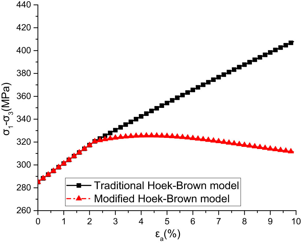
Comparison between the improved model and the traditional model.
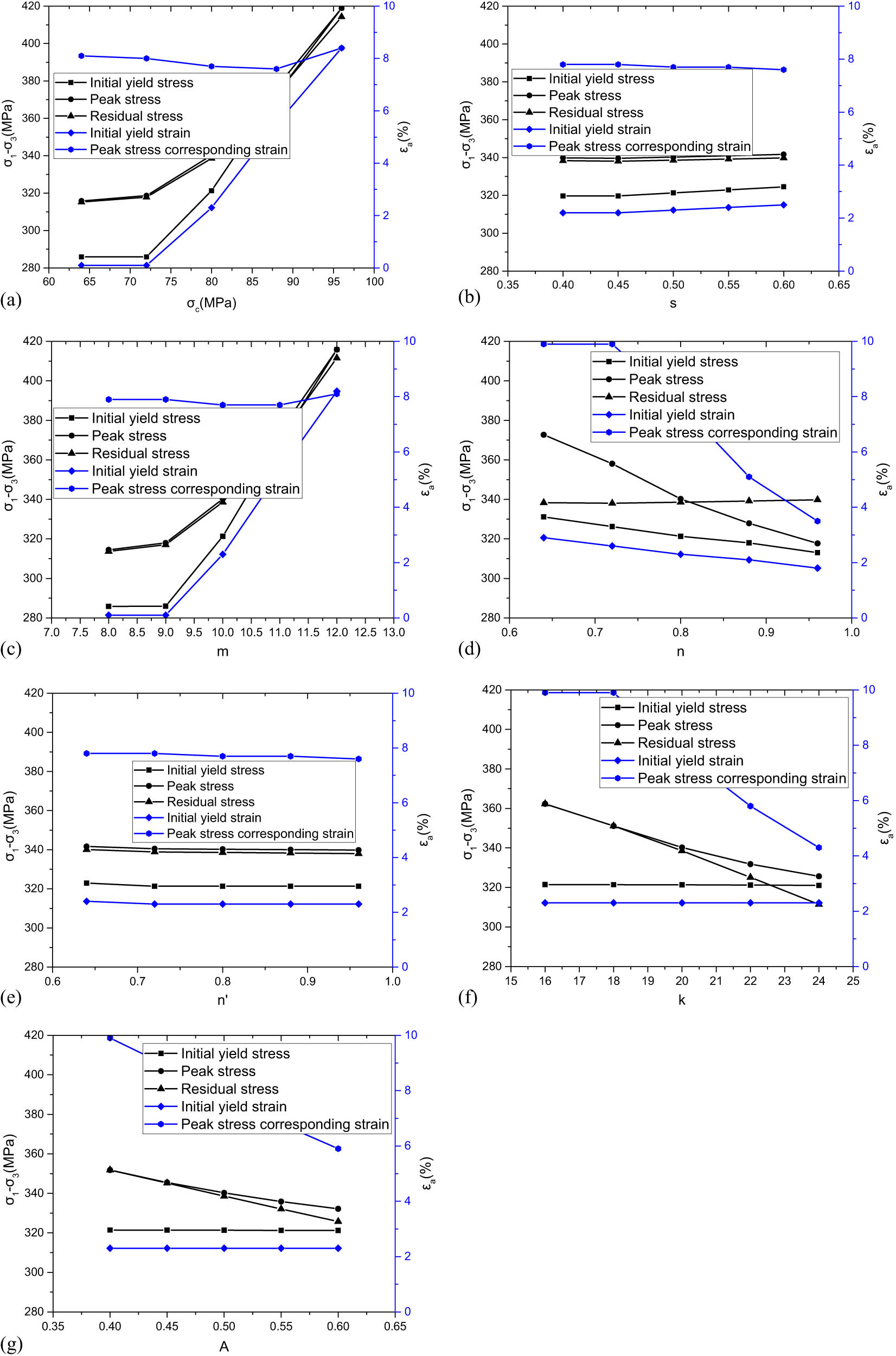
Multivariate calculation results. (a) Calculation results when
Calculation results when
| Value of
|
Initial yield | Peak value | Residual stress (MPa) | ||
|---|---|---|---|---|---|
| Stress (MPa) | Strain (%) | Stress (MPa) | Strain (%) | ||
| 0.40 | 285.54 | 0.1 | 302.37 | 8.4 | 302.15 |
| 0.45 | 285.74 | 0.1 | 309.73 | 8.2 | 309.29 |
| 0.50 | 321.31 | 2.3 | 340.25 | 7.7 | 338.59 |
| 0.55 | — | — | 444.92 | 10.0 | 444.92 |
| 0.60 | — | — | 444.92 | 10.0 | 444.92 |
The comparison of calculation results between the modified model and the traditional model is shown in Figure 1. From the figure, it is evident that the traditional Hoek–Brown model fails to account for the strain softening effect of the material, whereas the modified Hoek–Brown model proposed in this article can describe the mechanical behavior of materials, including initial elastic deformation, subsequent hardening, and eventual softening. This clearly aligns more closely with the actual mechanical properties of rock-like materials.
When the model parameters change, the modified model calculates the initial yield stress, peak stress, and residual stress, as shown in Figure 2. As depicted in Figure 2(a), the parameter
As shown in Figure 2(f), parameter k has no effect on the initial yield stress and its corresponding strain. When k = 16, the peak stress equals the residual stress, both of which are greater than the initial yield stress, indicating no strain softening in the material. When k = 20, the peak stress is slightly greater than the residual stress, with the residual stress still greater than the initial yield stress, indicating mild strain softening in the material. When k = 22, the peak stress exceeds the initial yield stress, and the initial yield stress exceeds the residual stress, indicating significant strain softening in the material. It is evident that the parameter k effectively controls the rate of strain softening. As shown in Figure 2(g), the parameter A has no effect on the initial yield stress and its corresponding strain. With increasing A, the softening effect becomes more pronounced, which is determined by the physical meaning of A. As shown in Table 1, A represents the proportion of plastic shear strain in the equivalent plastic strain causing material degradation or damage. The multivariate calculations adopt a model where volumetric strain is zero; hence, a larger A indicates faster material damage development, resulting in a more pronounced softening effect accordingly.
5 Engineering applications of the modified model
The Dianzhong Diversion Project, a pivotal water diversion initiative undertaken by the state, addresses the pressing water scarcity in the central region of Yunnan Province [30]. As shown in Figure 3, this monumental engineering endeavor encompasses a water receiving area spanning 3.69 × 10⁴ km2, with an annual average diversion volume reaching 34.03 × 10⁹ m3. Within the tunnel which extends over a length of 102.74 km, particularly in the Dali city segment, the project encounters the challenges posed by red bed soft rocks. The construction of tunnels through these geological formations has been fraught with varying degrees of soft rock deformation, with the deformation near the exit section of the tunnel emerging as a particularly exemplary case. The project’s complexity is further amplified by the intricate topography and geological conditions. This study focuses on a segment of a tunnel exit in the Dianzhong Diversion Project, analyzing deformation characteristics of the tunnel and the surrounding rocks using the modified Hoek–Brown model, combined with field monitoring data. The findings provide valuable insights for the construction of subsequent soft rock tunnels.
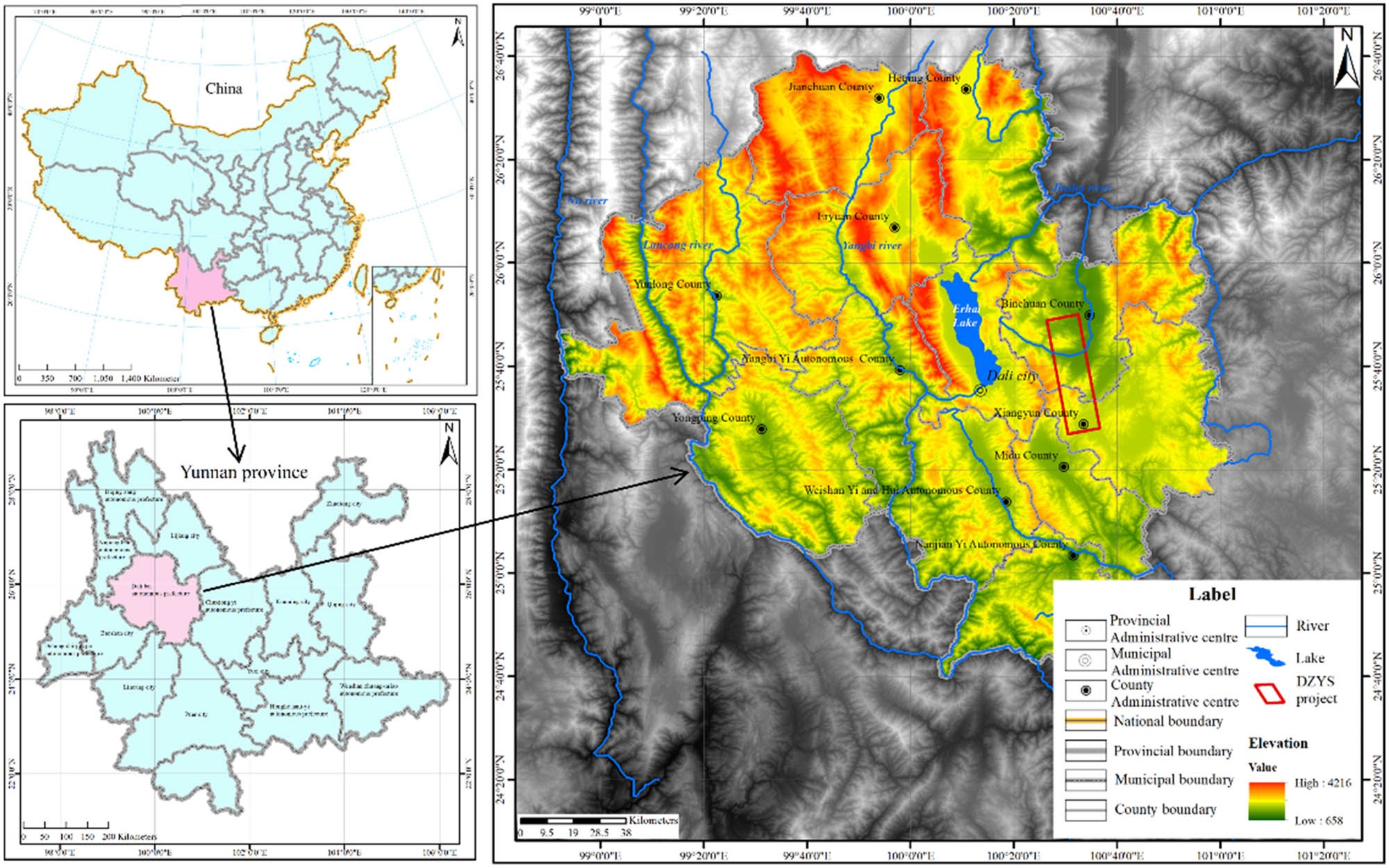
Location map of background engineering.
During tunnel excavation, stress redistributes in the surrounding rock mass. As stress conditions change, rock masses within a certain range around the tunnel may exceed their ultimate strength. Additionally, due to the weakening of rock strength on the tunnel’s inner side, its load-bearing capacity decreases. This results in increased loads on adjacent rock masses, causing deformation and plastic zones to expand outward until the rock masses within the load-bearing zone reach their ultimate stress state. Considering the softening effect of rock masses, the mechanical properties of the surrounding rock decrease, making it easier for the rock masses to reach their ultimate stress state, thereby further expanding the plastic zone outward from the tunnel and affecting the stability of the tunnel surrounding the rock mass.
The tunnel is located in a red soft rock region where significant surrounding rock deformations can occur. Considering that the tunnel depth is much greater than its diameter, and surface topography has minimal impact, the computational model adopts a quasi-three-dimensional approach. To minimize boundary effects, the model ensures that boundaries are more than five times the tunnel diameter away from the tunnel. The computational model, constructed using hexahedral elements, as shown in Figure 4(a), comprises over 60,000 elements. Initial support measures are designed for Class V surrounding rock conditions, with the specific support structure depicted in Figure 4(b).
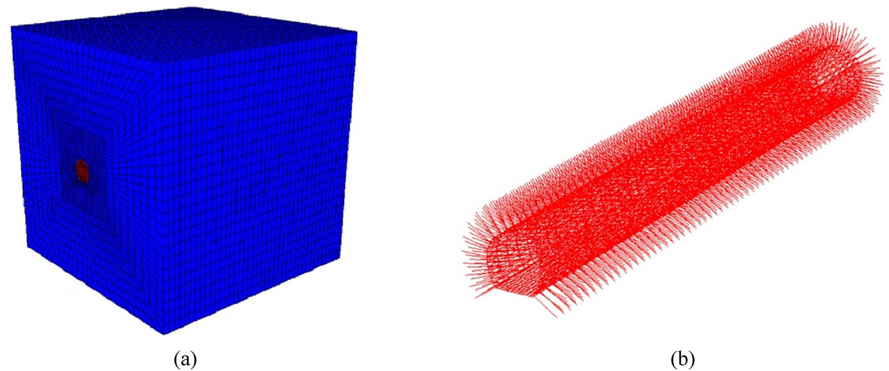
Computation model. (a) Tunnel and surrounding rock model. (b) Tunnel support model.
The total displacements and maximum principal stresses calculated using both the traditional Hoek–Brown model and the modified Hoek–Brown model proposed in this article are shown in Figure 5(a)–(d), and the comparison with field measurements is presented in Table 4. According to the calculations using the traditional Hoek–Brown model, which does not account for rock softening, the most significant displacements occur at the bottom of the tunnel, reaching up to 6.16 cm. When considering rock softening effects using the modified Hoek–Brown model, the maximum displacement calculated is 15.13 cm, still located at the tunnel bottom. Compared to the scenario without considering rock softening, this represents an increase of nearly 9 cm, a percentage increase of 146%. This clearly indicates a substantial difference in displacements between considering rock softening and not considering it. Furthermore, when using the traditional Hoek–Brown model, the maximum principal stress around the tunnel ranges from 0.98 to 21.63 MPa, whereas with the modified Hoek–Brown model considering rock softening effects, the maximum principal stress ranges from 1.14 to 18 MPa. This directly illustrates that considering rock softening reduces the range of principal stress distribution around the tunnel, thereby improving the stress conditions and promoting the stability of the surrounding rock mass.
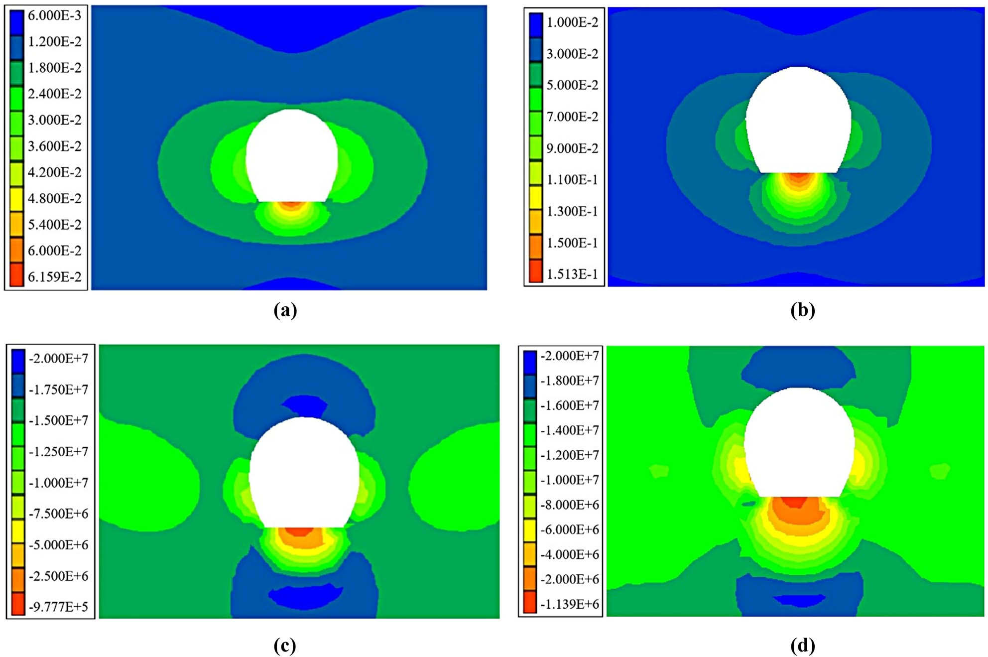
Comparison of results between the traditional Hoek–Brown model and the modified Hoek–Brown model. (a) Total displacement calculated by the traditional model (m). (b) Total displacement calculated by the modified model (m). (c) Maximum principal stress calculated by the traditional model (Pa). (d) Maximum principal stress calculated by the modified model (Pa).
Comparison between calculation results and monitoring results
| Position | Displacement at the bottom of the tunnel (mm) | Stress at the bottom of the tunnel (MPa) | Stress at the top of the tunnel (MPa) |
|---|---|---|---|
| Monitor value | 138.47 | 1.28 | 14.32 |
| Traditional model calculation values | 61.6 | 0.98 | 21.63 |
| Modified model calculation values | 151.3 | 1.14 | 18.00 |
The displacements and stresses obtained from the traditional Hoek–Brown model, the modified Hoek–Brown model, and on-site monitoring results are compared in Table 4. As shown in the table, for soft rock tunnels, both the displacements around the tunnel perimeter and the stresses obtained from the modified Hoek–Brown model are much more consistent with engineering practice compared to those from the traditional Hoek–Brown model. This discrepancy primarily arises because the surrounding rock mass undergoes significant deformation in the case studies, triggering strain softening effects. The traditional Hoek–Brown model, which only considers strain hardening effects and neglects strain softening of the rock mass, therefore produces results that diverge significantly from reality.
6 Conclusions
In order to simultaneously consider strain hardening and softening effects, this study proposes a modified Hoek–Brown model based on the traditional Hoek–Brown model. The modified model addresses numerical singularity and convergence challenges encountered during its implementation and applies the modified model to engineering practice. The main conclusions are as follows:
The traditional Hoek Brown model can only consider strain hardening effects. Improving the traditional Hoek–Brown model by introducing internal variables is feasible, enabling the modified Hoek–Brown model to simultaneously account for strain hardening and strain softening effects of materials.
The function smoothing method proposed in this article effectively resolves numerical singularity and convergence issues in the implementation of the modified Hoek–Brown model. It is suggested that this method can be applied to similar cases where the yield function has corner points in the stress space in the future.
For soft rock tunnels, when significant displacements occur in the surrounding rock mass, both perimeter displacements and stresses predicted by the modified Hoek–Brown model are much closer to engineering reality compared to those predicted by the traditional Hoek–Brown model, which exhibits an error as high as 146%.
Acknowledgments
The Major Science and Technology Special Plan of Yunnan Province Science and Technology Department (Grant No. 202002AF080003) is greatly appreciated for providing financial support to this work. This work was completed on the basis of the open-source finite element software FreeFEM, and the work done by the developers is greatly appreciated.
-
Funding information: This work was financially supported by The Major Science and Technology Special Plan of Yunnan Province Science and Technology Department (Grant No. 202002AF080003).
-
Author contributions: LZ and SFL developed the research frameworks. LZ and ZHT proposed the modified model. YTX and YLF wrote the corresponding program for the modified model. JM and YY validated the effectiveness of the modified model. DYS and YT applied the modified model for practical engineering. LZ and BXW wrote the initial draft. ZHT and YTX revised the manuscript. The authors applied the SDC approach for the sequence of authors.
-
Conflict of interest: The authors state no conflict of interest.
References
[1] Geng D, Dai N, Guo P, Zhou S, Di H. Implicit numerical integration of highly nonlinear plasticity models. Comput Geotech. 2021;132:103961. 10.1016/j.compgeo.2020.103961.Search in Google Scholar
[2] Sun Z, Zhang D, Fang Q, Dui G, Chu Z. Analytical solutions for deep tunnels in strain-softening rocks modeled by different elastic strain definitions with the unified strength theory. Sci China Technol Sci. 2022;65(10):2503–19. 10.1007/s11431-022-2158-9.Search in Google Scholar
[3] Li J, Shen C, He X, Zheng X, Yuan J. Numerical solution for circular tunnel excavated in strain-softening rock masses considering damaged zone. Sci Rep. 2022;12(1):4465. 10.1038/s41598-022-08531-3.Search in Google Scholar PubMed PubMed Central
[4] Gao W, Hu C, He T, Chen X, Zhou C, Cui S. Study on constitutive model of fractured rock mass based on statistical strength theory. Rock Soil Mech. 2020;41(7):2179–88. 10.16285/j.rsm.2019.1673 (in Chinese).Search in Google Scholar
[5] Wang Z, Zhu Z, Zhu S. Thermo-mechanical-water migration coupled plastic constitutive model of rock subjected to freeze-thaw. Cold Reg Sci Technol. 2019;161:71–80. 10.1016/j.coldregions.2019.03.001.Search in Google Scholar
[6] Zhang H, Meng X, Liu X. Establishment of constitutive model and analysis of damage characteristics of frozen-thawed rock under load. Arab J Geosci. 2021;14:1–13. 10.1007/s12517-021-07598-y.Search in Google Scholar
[7] Yang P, Wu X, Chen J. Elastic and plastic-flow damage constitutive model of rock based on conventional triaxial compression test. Int J Heat Technol. 2018;36(3):627–35. 10.18280/ijht.360320.Search in Google Scholar
[8] Wei X, Zhao B, Ji C, Liu Z, Zhang Z. Elastoplastic augmented virtual internal bond modeling for rock: A fracture‐plasticity combined constitutive model. Int J Numer Anal Methods Geomech. 2023;47(8):1331–48. 10.1002/nag.3516.Search in Google Scholar
[9] Chen S, Qiao C. Composite damage constitutive model of jointed rock mass considering crack propagation length and joint friction effect. Arab J Geosci. 2018;11:1–11. 10.1007/s12517-018-3643-y.Search in Google Scholar
[10] Li T, Lyu L, Zhang S, Sun J. Development and application of a statistical constitutive model of damaged rock affected by the load-bearing capacity of damaged elements. J Zhejiang Univ-Sci A (Appl Phys Eng). 2015;8:644–55. 10.1631/jzus.A1500034.Search in Google Scholar
[11] Xie S, Lin H, Wang Y, Cao R, Yong R, Du S, et al. Nonlinear shear constitutive model for peak shear-type joints based on improved Harris damage function. Arch Civ Mech Eng. 2020;20:1–14. 10.1007/s43452-020-00097-z.Search in Google Scholar
[12] Xin J, Jiang Q, Liu Q, Zheng H, Li S. A shear constitutive model and experimental demonstration considering dual void portion and solid skeleton portion of rock. Eng Fract Mech. 2023;281:109066. 10.1016/j.engfracmech.2023.109066.Search in Google Scholar
[13] Xie S, Han Z, Hu H, Lin H. Application of a novel constitutive model to evaluate the shear deformation of discontinuity. Eng Geol. 2022;304:106693. 10.1016/j.enggeo.2022.106693.Search in Google Scholar
[14] Xie S, Lin H, Chen Y. New constitutive model based on disturbed state concept for shear deformation of rock joints. Arch Civ Mech Eng. 2022;23(1):26. 10.1007/s43452-022-00560-z.Search in Google Scholar
[15] Chen Y, Lin H, Wang Y, Xie S, Zhao Y, Yong W. Statistical damage constitutive model based on the Hoek–Brown criterion. Arch Civ Mech Eng. 2021;21:1–9. 10.1007/s43452-021-00270-y.Search in Google Scholar
[16] Bian K, Liu J, Zhang W, Zheng X, Ni S, Liu Z. Mechanical behavior and damage constitutive model of rock subjected to water-weakening effect and uniaxial loading. Rock Mech Rock Eng. 2019;52:97–106. 10.1007/s00603-018-1580-4.Search in Google Scholar
[17] Wen Z, Tian L, Jiang Y, Zuo Y, Meng F, Dong Y, et al. Research on damage constitutive model of inhomogeneous rocks based on strain energy density. Chin J Rock Mech Eng. 2019;7:1332–43. 10.13722/j.cnki.jrme.2018.1125 (in Chinese).Search in Google Scholar
[18] Qu D, Li D, Li X, Yi L, Xu K. Damage evolution mechanism and constitutive model of freeze-thaw yellow sandstone in acidic environment. Cold Reg Sci Technol. 2018;155:174–83. 10.1016/j.coldregions.2018.07.012.Search in Google Scholar
[19] Fang W, Jiang N, Luo X. Establishment of damage statistical constitutive model of loaded rock and method for determining its parameters under freeze-thaw condition. Cold Reg Sci Technol. 2019;160:31–8. 10.1016/j.coldregions.2019.01.004.Search in Google Scholar
[20] Jiang H, Liu D, Zhao B, Li D. Nonlinear creep constitutive model of rock under high confining pressure and high water pressure. J Min Saf Eng. 2014;31(2):284–91 (in Chinese).Search in Google Scholar
[21] Lin H, Liang L, Chen Y, Cao R. A damage constitutive model of rock subjected to freeze-thaw cycles based on lognormal distribution. Adv Civ Eng. 2021;2021:1–8. 10.1155/2021/6658915.Search in Google Scholar
[22] Ma Q, Liu Z, Qin Y, Tian J, Wang J. Rock plastic-damage constitutive model based on energy dissipation. Rock Soil Mech. 2021;42(05):1210–20. 10.16285/j.rsm.2020.1091 (in Chinese).Search in Google Scholar
[23] Meng X, Zhang H, Liu X. Rock damage constitutive model based on the modified logistic equation under freeze–thaw and load conditions. J Cold Reg Eng. 2021;35(4):04021016. 10.1061/(ASCE)CR.1943-5495.0000268.Search in Google Scholar
[24] Leng D, Shi W, Liang F, Li H, Yan L. Stability and deformation evolution analysis of karstified slope subjected to underground mining based on Hoek–Brown failure criterion. Bull Eng Geol Environ. 2023;82(5):174. 10.1007/s10064-023-03211-6.Search in Google Scholar
[25] Wang J, Wu S, Cheng H, Sun J, Wang X, Shen Y. A generalized nonlinear three-dimensional Hoek-Brown failure criterion. J Rock Mech Geotech Eng. 2024;16(8):3149–64. 10.1016/j.jrmge.2023.10.022.Search in Google Scholar
[26] He L, Zhao Y, Yin L, Zhong D, Xiong H, Chen S, et al. Research on a non-synchronous coordinated reduction method for slopes based on the Hoek–Brown criterion and acoustic testing technology. Sustainability. 2023;15(21):15516. 10.3390/su152115516.Search in Google Scholar
[27] Liu J, Jiang Q, Dias D, Tao C. Probability quantification of GSI and D in Hoek–Brown criterion using Bayesian inversion and ultrasonic test in rock mass. Rock Mech Rock Eng. 2023;56(10):7701–19. 10.1016/j.jrmge.2023.06.004.Search in Google Scholar
[28] Cai W, Su C, Zhu H, Liang W, Ma Y, Xu J, et al. Elastic–plastic response of a deep tunnel excavated in 3D Hoek–Brown rock mass considering different approaches for obtaining the out-of-plane stress. Int J Rock Mech Min Sci. 2023;169:105425. 10.1016/j.ijrmms.2023.105425.Search in Google Scholar
[29] Zhong J, Hou C, Yang X. Three-dimensional face stability analysis of rock tunnels excavated in Hoek-Brown media with a novel multi-cone mechanism. Comput Geotech. 2023;154:105158. 10.1016/j.compgeo.2022.105158.Search in Google Scholar
[30] Yuan F, Bao C, Wang M, Su W, Zhou J. Study on large deformation characteristics and control measures of red-bed soft rock tunnel. Chin J Undergr Space Eng. 2022;18(S1):332–40 + 349 (in Chinese).Search in Google Scholar
© 2025 the author(s), published by De Gruyter
This work is licensed under the Creative Commons Attribution 4.0 International License.
Articles in the same Issue
- Research Articles
- Seismic response and damage model analysis of rocky slopes with weak interlayers
- Multi-scenario simulation and eco-environmental effect analysis of “Production–Living–Ecological space” based on PLUS model: A case study of Anyang City
- Remote sensing estimation of chlorophyll content in rape leaves in Weibei dryland region of China
- GIS-based frequency ratio and Shannon entropy modeling for landslide susceptibility mapping: A case study in Kundah Taluk, Nilgiris District, India
- Natural gas origin and accumulation of the Changxing–Feixianguan Formation in the Puguang area, China
- Spatial variations of shear-wave velocity anomaly derived from Love wave ambient noise seismic tomography along Lembang Fault (West Java, Indonesia)
- Evaluation of cumulative rainfall and rainfall event–duration threshold based on triggering and non-triggering rainfalls: Northern Thailand case
- Pixel and region-oriented classification of Sentinel-2 imagery to assess LULC dynamics and their climate impact in Nowshera, Pakistan
- The use of radar-optical remote sensing data and geographic information system–analytical hierarchy process–multicriteria decision analysis techniques for revealing groundwater recharge prospective zones in arid-semi arid lands
- Effect of pore throats on the reservoir quality of tight sandstone: A case study of the Yanchang Formation in the Zhidan area, Ordos Basin
- Hydroelectric simulation of the phreatic water response of mining cracked soil based on microbial solidification
- Spatial-temporal evolution of habitat quality in tropical monsoon climate region based on “pattern–process–quality” – a case study of Cambodia
- Early Permian to Middle Triassic Formation petroleum potentials of Sydney Basin, Australia: A geochemical analysis
- Micro-mechanism analysis of Zhongchuan loess liquefaction disaster induced by Jishishan M6.2 earthquake in 2023
- Prediction method of S-wave velocities in tight sandstone reservoirs – a case study of CO2 geological storage area in Ordos Basin
- Ecological restoration in valley area of semiarid region damaged by shallow buried coal seam mining
- Hydrocarbon-generating characteristics of Xujiahe coal-bearing source rocks in the continuous sedimentary environment of the Southwest Sichuan
- Hazard analysis of future surface displacements on active faults based on the recurrence interval of strong earthquakes
- Structural characterization of the Zalm district, West Saudi Arabia, using aeromagnetic data: An approach for gold mineral exploration
- Research on the variation in the Shields curve of silt initiation
- Reuse of agricultural drainage water and wastewater for crop irrigation in southeastern Algeria
- Assessing the effectiveness of utilizing low-cost inertial measurement unit sensors for producing as-built plans
- Analysis of the formation process of a natural fertilizer in the loess area
- Machine learning methods for landslide mapping studies: A comparative study of SVM and RF algorithms in the Oued Aoulai watershed (Morocco)
- Chemical dissolution and the source of salt efflorescence in weathering of sandstone cultural relics
- Molecular simulation of methane adsorption capacity in transitional shale – a case study of Longtan Formation shale in Southern Sichuan Basin, SW China
- Evolution characteristics of extreme maximum temperature events in Central China and adaptation strategies under different future warming scenarios
- Estimating Bowen ratio in local environment based on satellite imagery
- 3D fusion modeling of multi-scale geological structures based on subdivision-NURBS surfaces and stratigraphic sequence formalization
- Comparative analysis of machine learning algorithms in Google Earth Engine for urban land use dynamics in rapidly urbanizing South Asian cities
- Study on the mechanism of plant root influence on soil properties in expansive soil areas
- Simulation of seismic hazard parameters and earthquakes source mechanisms along the Red Sea rift, western Saudi Arabia
- Tectonics vs sedimentation in foredeep basins: A tale from the Oligo-Miocene Monte Falterona Formation (Northern Apennines, Italy)
- Investigation of landslide areas in Tokat-Almus road between Bakımlı-Almus by the PS-InSAR method (Türkiye)
- Predicting coastal variations in non-storm conditions with machine learning
- Cross-dimensional adaptivity research on a 3D earth observation data cube model
- Geochronology and geochemistry of late Paleozoic volcanic rocks in eastern Inner Mongolia and their geological significance
- Spatial and temporal evolution of land use and habitat quality in arid regions – a case of Northwest China
- Ground-penetrating radar imaging of subsurface karst features controlling water leakage across Wadi Namar dam, south Riyadh, Saudi Arabia
- Rayleigh wave dispersion inversion via modified sine cosine algorithm: Application to Hangzhou, China passive surface wave data
- Fractal insights into permeability control by pore structure in tight sandstone reservoirs, Heshui area, Ordos Basin
- Debris flow hazard characteristic and mitigation in Yusitong Gully, Hengduan Mountainous Region
- Research on community characteristics of vegetation restoration in hilly power engineering based on multi temporal remote sensing technology
- Identification of radial drainage networks based on topographic and geometric features
- Trace elements and melt inclusion in zircon within the Qunji porphyry Cu deposit: Application to the metallogenic potential of the reduced magma-hydrothermal system
- Pore, fracture characteristics and diagenetic evolution of medium-maturity marine shales from the Silurian Longmaxi Formation, NE Sichuan Basin, China
- Study of the earthquakes source parameters, site response, and path attenuation using P and S-waves spectral inversion, Aswan region, south Egypt
- Source of contamination and assessment of potential health risks of potentially toxic metal(loid)s in agricultural soil from Al Lith, Saudi Arabia
- Regional spatiotemporal evolution and influencing factors of rural construction areas in the Nanxi River Basin via GIS
- An efficient network for object detection in scale-imbalanced remote sensing images
- Effect of microscopic pore–throat structure heterogeneity on waterflooding seepage characteristics of tight sandstone reservoirs
- Environmental health risk assessment of Zn, Cd, Pb, Fe, and Co in coastal sediments of the southeastern Gulf of Aqaba
- A modified Hoek–Brown model considering softening effects and its applications
- Evaluation of engineering properties of soil for sustainable urban development
- The spatio-temporal characteristics and influencing factors of sustainable development in China’s provincial areas
- Application of a mixed additive and multiplicative random error model to generate DTM products from LiDAR data
- Gold vein mineralogy and oxygen isotopes of Wadi Abu Khusheiba, Jordan
- Prediction of surface deformation time series in closed mines based on LSTM and optimization algorithms
- 2D–3D Geological features collaborative identification of surrounding rock structural planes in hydraulic adit based on OC-AINet
- Spatiotemporal patterns and drivers of Chl-a in Chinese lakes between 1986 and 2023
- Land use classification through fusion of remote sensing images and multi-source data
- Nexus between renewable energy, technological innovation, and carbon dioxide emissions in Saudi Arabia
- Analysis of the spillover effects of green organic transformation on sustainable development in ethnic regions’ agriculture and animal husbandry
- Factors impacting spatial distribution of black and odorous water bodies in Hebei
- Large-scale shaking table tests on the liquefaction and deformation responses of an ultra-deep overburden
- Impacts of climate change and sea-level rise on the coastal geological environment of Quang Nam province, Vietnam
- Reservoir characterization and exploration potential of shale reservoir near denudation area: A case study of Ordovician–Silurian marine shale, China
- Seismic prediction of Permian volcanic rock reservoirs in Southwest Sichuan Basin
- Application of CBERS-04 IRS data to land surface temperature inversion: A case study based on Minqin arid area
- Geological characteristics and prospecting direction of Sanjiaoding gold mine in Saishiteng area
- Research on the deformation prediction model of surrounding rock based on SSA-VMD-GRU
- Geochronology, geochemical characteristics, and tectonic significance of the granites, Menghewula, Southern Great Xing’an range
- Hazard classification of active faults in Yunnan base on probabilistic seismic hazard assessment
- Characteristics analysis of hydrate reservoirs with different geological structures developed by vertical well depressurization
- Estimating the travel distance of channelized rock avalanches using genetic programming method
- Landscape preferences of hikers in Three Parallel Rivers Region and its adjacent regions by content analysis of user-generated photography
- New age constraints of the LGM onset in the Bohemian Forest – Central Europe
- Characteristics of geological evolution based on the multifractal singularity theory: A case study of Heyu granite and Mesozoic tectonics
- Soil water content and longitudinal microbiota distribution in disturbed areas of tower foundations of power transmission and transformation projects
- Oil accumulation process of the Kongdian reservoir in the deep subsag zone of the Cangdong Sag, Bohai Bay Basin, China
- Investigation of velocity profile in rock–ice avalanche by particle image velocimetry measurement
- Optimizing 3D seismic survey geometries using ray tracing and illumination modeling: A case study from Penobscot field
- Sedimentology of the Phra That and Pha Daeng Formations: A preliminary evaluation of geological CO2 storage potential in the Lampang Basin, Thailand
- Improved classification algorithm for hyperspectral remote sensing images based on the hybrid spectral network model
- Map analysis of soil erodibility rates and gully erosion sites in Anambra State, South Eastern Nigeria
- Identification and driving mechanism of land use conflict in China’s South-North transition zone: A case study of Huaihe River Basin
- Evaluation of the impact of land-use change on earthquake risk distribution in different periods: An empirical analysis from Sichuan Province
- A test site case study on the long-term behavior of geotextile tubes
- An experimental investigation into carbon dioxide flooding and rock dissolution in low-permeability reservoirs of the South China Sea
- Detection and semi-quantitative analysis of naphthenic acids in coal and gangue from mining areas in China
- Comparative effects of olivine and sand on KOH-treated clayey soil
- YOLO-MC: An algorithm for early forest fire recognition based on drone image
- Earthquake building damage classification based on full suite of Sentinel-1 features
- Potential landslide detection and influencing factors analysis in the upper Yellow River based on SBAS-InSAR technology
- Assessing green area changes in Najran City, Saudi Arabia (2013–2022) using hybrid deep learning techniques
- An advanced approach integrating methods to estimate hydraulic conductivity of different soil types supported by a machine learning model
- Hybrid methods for land use and land cover classification using remote sensing and combined spectral feature extraction: A case study of Najran City, KSA
- Streamlining digital elevation model construction from historical aerial photographs: The impact of reference elevation data on spatial accuracy
- Analysis of urban expansion patterns in the Yangtze River Delta based on the fusion impervious surfaces dataset
- A metaverse-based visual analysis approach for 3D reservoir models
- Late Quaternary record of 100 ka depositional cycles on the Larache shelf (NW Morocco)
- Integrated well-seismic analysis of sedimentary facies distribution: A case study from the Mesoproterozoic, Ordos Basin, China
- Study on the spatial equilibrium of cultural and tourism resources in Macao, China
- Urban road surface condition detecting and integrating based on the mobile sensing framework with multi-modal sensors
- Application of improved sine cosine algorithm with chaotic mapping and novel updating methods for joint inversion of resistivity and surface wave data
- The synergistic use of AHP and GIS to assess factors driving forest fire potential in a peat swamp forest in Thailand
- Dynamic response analysis and comprehensive evaluation of cement-improved aeolian sand roadbed
- Rock control on evolution of Khorat Cuesta, Khorat UNESCO Geopark, Northeastern Thailand
- Gradient response mechanism of carbon storage: Spatiotemporal analysis of economic-ecological dimensions based on hybrid machine learning
- Comparison of several seismic active earth pressure calculation methods for retaining structures
- Mantle dynamics and petrogenesis of Gomer basalts in the Northwestern Ethiopia: A geochemical perspective
- Study on ground deformation monitoring in Xiong’an New Area from 2021 to 2023 based on DS-InSAR
- Paleoenvironmental characteristics of continental shale and its significance to organic matter enrichment: Taking the fifth member of Xujiahe Formation in Tianfu area of Sichuan Basin as an example
- Equipping the integral approach with generalized least squares to reconstruct relict channel profile and its usage in the Shanxi Rift, northern China
- InSAR-driven landslide hazard assessment along highways in hilly regions: A case-based validation approach
- Attribution analysis of multi-temporal scale surface streamflow changes in the Ganjiang River based on a multi-temporal Budyko framework
- Maps analysis of Najran City, Saudi Arabia to enhance agricultural development using hybrid system of ANN and multi-CNN models
- Hybrid deep learning with a random forest system for sustainable agricultural land cover classification using DEM in Najran, Saudi Arabia
- Long-term evolution patterns of groundwater depth and lagged response to precipitation in a complex aquifer system: Insights from Huaibei Region, China
- Remote sensing and machine learning for lithology and mineral detection in NW, Pakistan
- Spatial–temporal variations of NO2 pollution in Shandong Province based on Sentinel-5P satellite data and influencing factors
- 10.1515/geo-2025-0901
- Review Articles
- Humic substances influence on the distribution of dissolved iron in seawater: A review of electrochemical methods and other techniques
- Applications of physics-informed neural networks in geosciences: From basic seismology to comprehensive environmental studies
- Ore-controlling structures of granite-related uranium deposits in South China: A review
- Shallow geological structure features in Balikpapan Bay East Kalimantan Province – Indonesia
- A review on the tectonic affinity of microcontinents and evolution of the Proto-Tethys Ocean in Northeastern Tibet
- Special Issue: Natural Resources and Environmental Risks: Towards a Sustainable Future - Part II
- Depopulation in the Visok micro-region: Toward demographic and economic revitalization
- Special Issue: Geospatial and Environmental Dynamics - Part II
- Advancing urban sustainability: Applying GIS technologies to assess SDG indicators – a case study of Podgorica (Montenegro)
- Spatiotemporal and trend analysis of common cancers in men in Central Serbia (1999–2021)
- Minerals for the green agenda, implications, stalemates, and alternatives
- Spatiotemporal water quality analysis of Vrana Lake, Croatia
- Functional transformation of settlements in coal exploitation zones: A case study of the municipality of Stanari in Republic of Srpska (Bosnia and Herzegovina)
- Hypertension in AP Vojvodina (Northern Serbia): A spatio-temporal analysis of patients at the Institute for Cardiovascular Diseases of Vojvodina
- Regional patterns in cause-specific mortality in Montenegro, 1991–2019
- Spatio-temporal analysis of flood events using GIS and remote sensing-based approach in the Ukrina River Basin, Bosnia and Herzegovina
- Flash flood susceptibility mapping using LiDAR-Derived DEM and machine learning algorithms: Ljuboviđa case study, Serbia
- Geocultural heritage as a basis for geotourism development: Banjska Monastery, Zvečan (Serbia)
- Assessment of groundwater potential zones using GIS and AHP techniques – A case study of the zone of influence of Kolubara Mining Basin
- Impact of the agri-geographical transformation of rural settlements on the geospatial dynamics of soil erosion intensity in municipalities of Central Serbia
- Where faith meets geomorphology: The cultural and religious significance of geodiversity explored through geospatial technologies
- Applications of local climate zone classification in European cities: A review of in situ and mobile monitoring methods in urban climate studies
- Complex multivariate water quality impact assessment on Krivaja River
- Ionization hotspots near waterfalls in Eastern Serbia’s Stara Planina Mountain
- Shift in landscape use strategies during the transition from the Bronze age to Iron age in Northwest Serbia
- Assessing the geotourism potential of glacial lakes in Plav, Montenegro: A multi-criteria assessment by using the M-GAM model
- Flash flood potential index at national scale: Susceptibility assessment within catchments