Establishing breather and N-soliton solutions for conformable Klein–Gordon equation
-
Muhammad Bilal
 ,
Fuad A. Awwad
,
Fuad A. Awwad

Abstract
This article develops and investigates the behavior of soliton solutions for the spatiotemporal conformable Klein–Gordon equation (CKGE), a well-known mathematical physics model that accounts for spinless pion and de-Broglie waves. To accomplish this task, we deploy an effective analytical method, namely, the modified extended direct algebraic method (mEDAM). This method first develops a nonlinear ordinary differential equation (NODE) through the use of a wave transformation. With the help of generalized Riccati NODE and balancing nonlinearity with the highest derivative term, it then assumes a finite series-form solution for the resulting NODE, from which four clusters of soliton solutions – generalized rational, trigonometric, exponential, and hyperbolic functions – are derived. Using contour and three-dimensional visuals, the behaviors of the soliton solutions – which are prominently described as dark kink, bright kink, breather, and other
1 Introduction
The prevalence of nonlinearity across the world emphasizes the necessity of creating nonlinear models, especially those that include fractional partial differential equations (FPDEs) and partial differential equations (PDEs) [1–4]. The wide range of applications in fluid dynamics, acoustics, image processing, vibration, biology, chemistry, physics, and control has attracted a lot of researchers to study nonlinear FPDEs [5–7]. Because of the great potential applications of these nonlinear FPDEs in various fields, researchers have invested a great deal of time and energy in finding analytical and numerical solutions [8–12]. Researchers have created a number of reliable and effective approaches to find and analyze exact solutions [13–17]. These methodologies encompass the first integral method [18], Laplace Adomian decomposition method [19,20], homotopy analysis method [21], natural transform decomposition method [22], modified simple equation method [23], (
Expanding on current methods to address nonlinear FPDEs (NFPDEs) is still a compelling and important area of research. Many NFPDEs, such as the impulsive fractional differential equations [29], the space-time fractional advection-dispersion equation [30–32], the fractional generalized Burgers’ equation [33], the fractional heat and mass-transport equation [34], and others, have been studied and solved as a result of the efforts of numerous researchers. Motivated by the ongoing research on addressing NFPDEs, this study aims to address conformable Klein–Gordon equation (CKGE) with mEDAM. The fractional generalization of the Klein–Gordon equation (KGE) is known as the CKGE. It substitutes fractional order conformable derivatives for the integer ordered derivatives in KGE, a relativistic wave equation related to Schrödinger equation. In mathematical physics, particularly in relativistic quantum mechanics, the spinless pion and de-Broglie waves are well explained by the KGE, a well-known model that was first developed in 1926 by Klein and Gordon as a relativistic equation for the function of a wave of an individual particle with zero spins. Numerous scientific domains, including quantum field theory, solid-state physics, and nonlinear optics, are found in this model. The equation has shown tremendous interest in the fields of condensed matter physics, solitons in a collisionless plasma, nonlinear wave equations, and recurrence of initial states. In a mathematical model, this equation is used in many scientific fields, including quantum field theory, nonlinear optics, and solid-state physics. This model is stated as follows [31]:
where
The fractional derivative operators
Before this research, several researchers have already used various analytical and numerical methods to investigate this equation in integer and fractional orders. For instance, the homotopy perturbation method was employed by Golmankhaneh et al. [44] to study fractional (FKGE). Khan et al. in [25] utilized the (
Nevertheless, the main goal of this study is to construct and examine new families of soliton solutions for CKGE using the enhanced mEDAM. Applications of these findings include quantum field theory, solid-state physics, nonlinear optics, and a deeper understanding of the dynamics of the CKGE. The proposed mEDAM is one of the most straightforward, important, and efficient algebraic procedures. Under the application of wave transformation and assumption of a series form solution, the strategic mEDAM transforms the CKGE into a system of nonlinear algebraic equations. Numerous soliton solutions in the form of generalized rational, trigonometric, exponential, and hyperbolic functions are produced when the resulting problem is solved using the Maple tool. From an academic perspective, soliton solutions for NFPDEs remain significant because they offer more depth and granularity than conventional solutions [54–57]. They are valuable in many technical and scientific fields due to their inherent stability and longevity. They provide effective information transfer and extensive concordance retention for nonlinear systems. To put it succinctly, the new findings of this study demonstrate the inventive character of our research by offering a unique and methodical discovery of numerous new soliton solutions. Soliton research is interested in studying nonlinear FPDEs that occur in quantum field theory, fluid dynamics, and optics. These soliton solutions offer a more profound understanding of the fundamental phenomena of CKGE in the associated scientific domains.
The rest of the article is organized as follows: Section 2 describes the CFD and proposed method’s methodology, Section 3 presents soliton solutions for the targeted biological population models, while Section 4 presents graphs of some soliton solutions and a discussion of our findings. Finally, a brief conclusion has been provided.
2 Methodology and materials
2.1 The definition of CFD
Several fractional derivative operators such as the Caputo operator, Riemann-Liouville operator, Atangana-Baleanu operator, Caputo-Fabrizio operator, CFD operator, and many more have been introduced by different mathematicians in literature [58–68]. Among these fractional derivative operators, the CFD operator is preferred by academics due to its predominant applications over other derivative operators. For instance, employing Khalil’s CFD and a matrix of Hessian, Lavín-Delgado et al. presented an innovative edge recognition technique that lowers noise and maintains image outlines regardless of dull contrasting situations [69]. Their method improved clarity of vision in edge identification and has potential uses in health care imaging for recognizing diseases, including cervical cancer along with medial cranial arterial ruptured arteries, hence enhancing clinical surveillance and the precision of diagnosis. One another advantage of CFD is that, unlike other derivative operators, it satisfies all derivative properties, particularly the chain rule, which is essential for our method for creating soliton solutions. By taking advantage of these beneficial properties of CFDs over alternative fractional derivative operators, explicit solutions for FPDEs can be derived. Notably, the soliton solutions of Eq. (1) cannot be obtained using alternative fractional derivative formulations because they violate the chain rule [70,71]. As a result, CFDs were introduced into Eq. (1). The study by Sarikaya et al. [72] defines the CFD operator of order
In this investigation, the following properties of this derivative are utilized:
where
2.2 The working procedure of mEDAM
The mEDAM is an efficient technique, which is utilized by many researchers to construct travelling wave and soliton solutions for nonlinear FPDEs [73]. The operational procedure of this proposed method is explained in this section [54]. Examine the FPDE of the structure:
where
The variable transformation of the form
(7)where
Next, we assume that (7) has the following solution:
(8)where
(9)where
We utilize MAPLE to solve this set of algebraic problems.
Family 1: When
and
Family 2: When
and
Family 3: When
and
Family 4: When
and
Family 5: When
and
Family 6: When
and
Family 7: When
Family 8: When
Family 9: When
Family 10: When
Family 11: When
and
Family 12: When
where
Similarly,
3 Execution of the mEDAM
In the present section, we use the suggested method mEDAM for constructing soliton solutions for CKGE stated in (1). We offer the subsequent transformation so that this approach may be expanded to solve (1):
where
Establishing the homogenous balance principle between
With the help of (9), we insert (12) into (11) which create a polynomial in
Case 1:
Case 2:
Case 3:
Case 4:
Assuming case 1, we obtain the following families of soliton solutions for (1):
Family 1.1: When
and
Family 1.2: When
and
Family 1.3: When
and
Family 1.4: When
and
Family 1.5: When
and
Family 1.6: When
and
Family 1.7: When
where
Assuming case 2, we obtain the following families of soliton solutions for (1):
Family 2.1: When
and
Family 2.2: When
and
Family 2.3: When
and
Family 2.4: When
and
Family 2.5: When
and
Family 2.6: When
and
Family 2.7: When
where
Assuming case 3, we obtain the following families of soliton solutions for (1):
Family 3.1: When
and
Family 3.2: When
and
Family 3.3: When
and
Family 3.4: When
and
Family 3.5: When
and
Family 3.6: When
and
Family 3.7: When
where
Assuming case 4, we obtain the following families of soliton solutions for (1):
Family 4.1: When
and
Family 4.2: When
and
Family 4.3: When
and
Family 4.4: When
and
Family 4.5: When
and
Family 4.6: When
and
Family 4.7: When
and
Family 4.8: When
where
4 Discussion and graphs
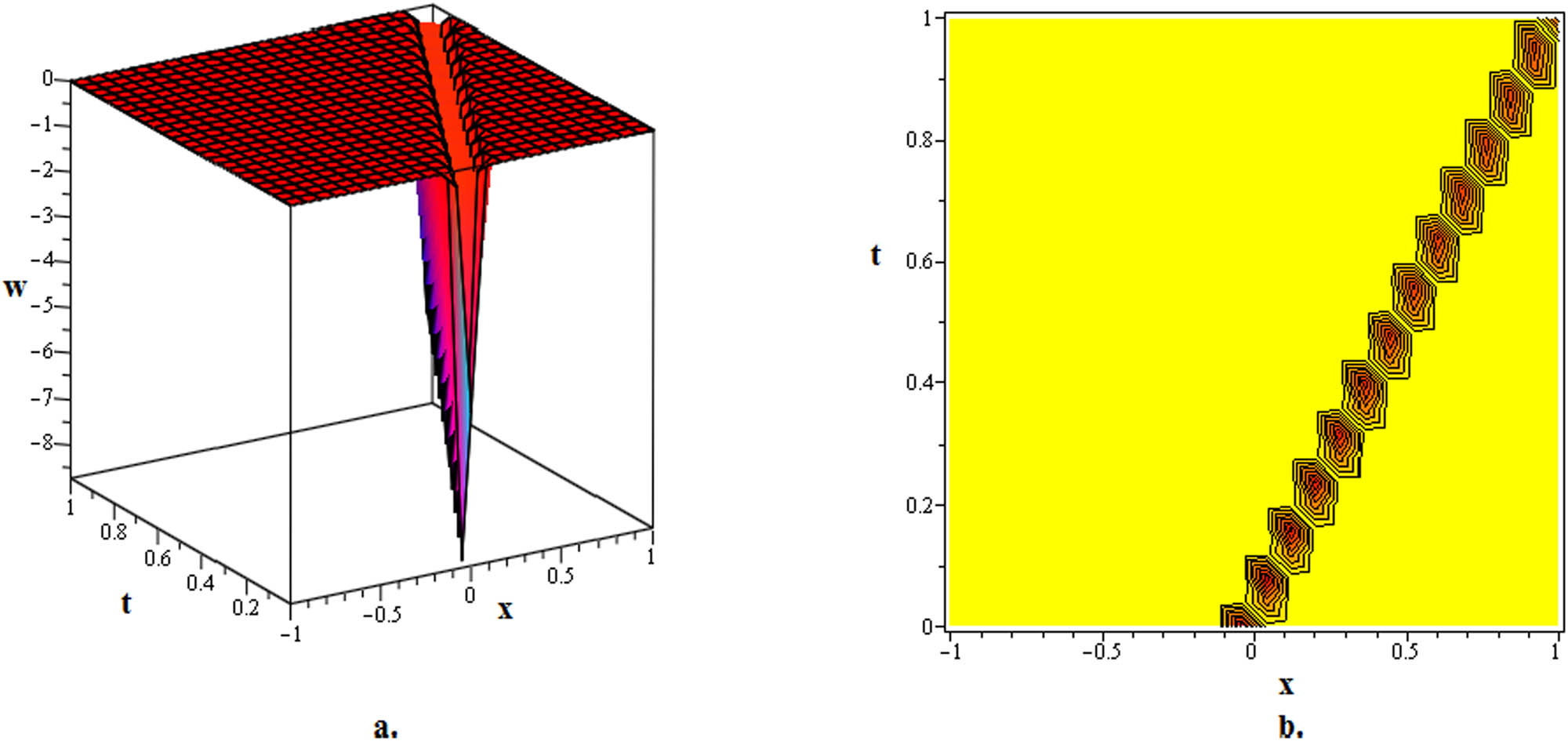
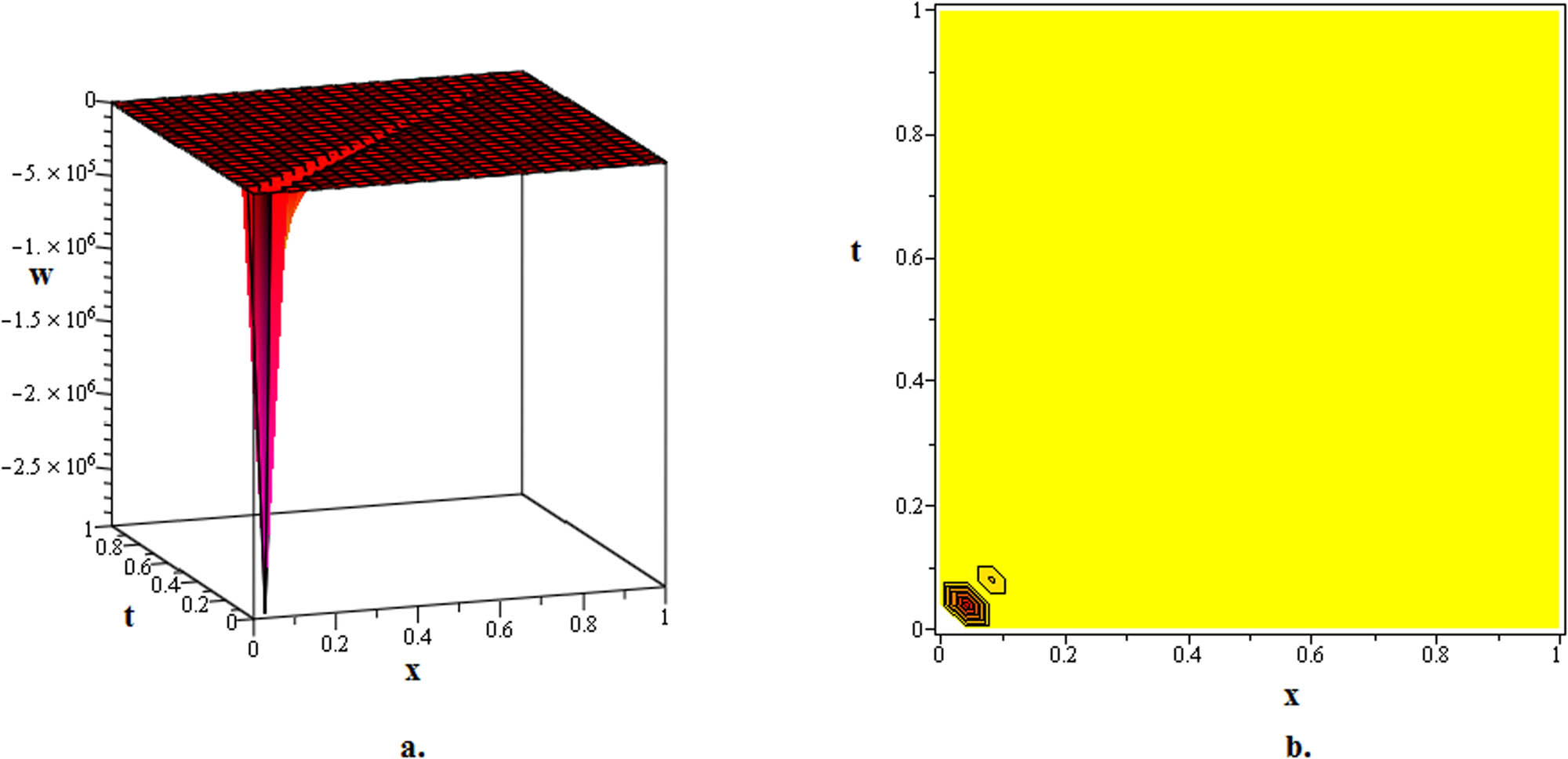
In this section, we graphically depict a number of wave patterns that were seen in the system that is being studied. By using the mEDAM, we were able to identify and display wave patterns in contour and 3D graphs. Predominantly, breather, dark kink, periodic, bright kinks, and other

The three-dimensional and contour graphics of the singular bright kink soliton solution
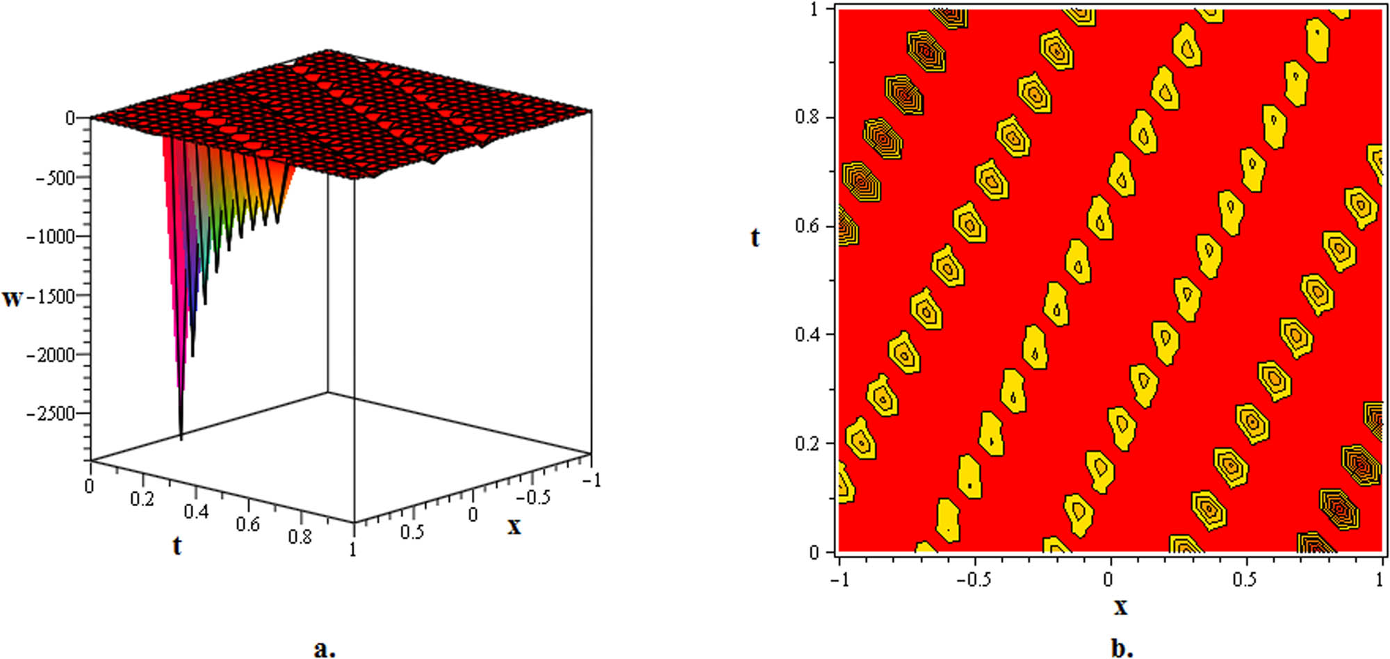
The three-dimensional and contour graphics of the dark soliton solution

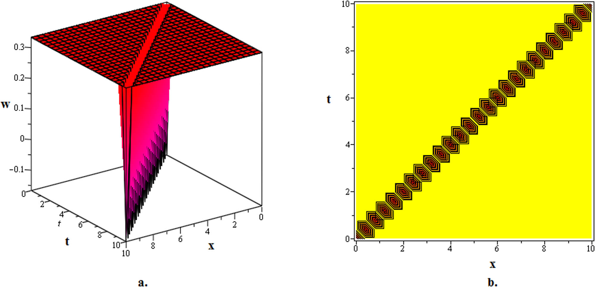
The three-dimensional and contour graphics of the dark soliton solution
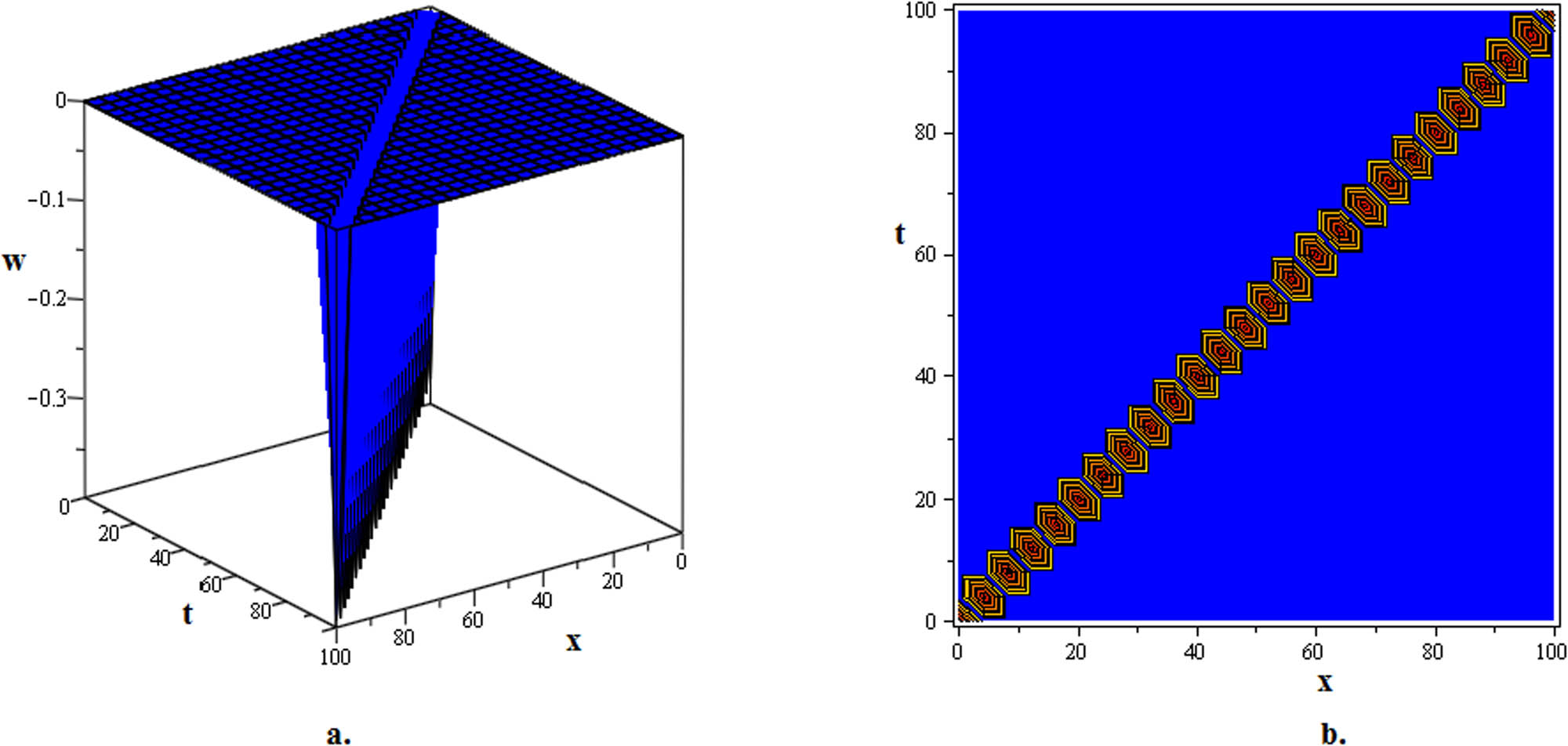
The three-dimensional and contour graphics of the breather dark soliton solution interacts with breather soliton solution
The three-dimensional and contour graphics of the breather dark soliton solution
The three-dimensional and contour graphics of the breather dark soliton solution
The three-dimensional and contour graphics of the dark soliton solution

The three-dimensional and contour graphics of the bell-shaped or dark kink soliton solution
5 Conclusion
We have used the upgraded mEDAM to comprehensively study the transmission of solitons in the CKGE, an established model in the fields of solid-state physics, quantum field theory, and nonlinear optics. Several dark kink, bright kink, breather, and other
Acknowledgments
Researchers Supporting Project number (RSPD2024R1060), King Saud University, Riyadh, Saudi Arabia.
-
Funding information: This project was funded by King Saud University, Riyadh, Saudi Arabia.
-
Author contributions: M.B. and J.I. conceptualized, analyzed data, and drafted the manuscript. R.A. supervised, designed methodologies, and oversaw experimentation. F.A.A managed administration and reviewed the manuscript. E.A.A.I. conducted experiments, analyzed data, and contributed to writing and visualizations. All authors have accepted responsibility for the entire content of this manuscript and approved its submission.
-
Conflict of interest: The authors state no conflict of interest.
-
Data availability statement: The datasets generated and/or analysed during the current study are available from the corresponding author on reasonable request.
References
[1] Bagchi BK. Partial differential equations for mathematical physicists. New York: Chapman and Hall/CRC; 2019. 10.1201/9780429276477Suche in Google Scholar
[2] Dehghan M, Manafian J, Saadatmandi A. Solving nonlinear fractional partial differential equations using the homotopy analysis method. Numer Methods Partial Differ Equ Int J. 2010;26(2):448–79. 10.1002/num.20460Suche in Google Scholar
[3] Ali R, Pan K, Ali A. Two generalized successive over relaxation methods for solving absolute value equations. Math Theory Appl. 2020;4(40):44–55. Suche in Google Scholar
[4] Ali R, Zhang Z, Ahmad H. Exploring soliton solutions in nonlinear spatiotemporal fractional quantum mechanics equations: an analytical study. Optical Quantum Electron. 2024;56:838. 10.1007/s11082-024-06370-2Suche in Google Scholar
[5] Kilbas AA, Srivastava HM, Trujillo JJ. Theory and applications of fractional differential equations. Vol. 204. The Netherlands: Elsevier; 2006. Suche in Google Scholar
[6] Miller KS, Ross B. An introduction to the fractional calculus and fractional differential equations. 1993. Suche in Google Scholar
[7] Han PF, Zhang Y, Jin CH. Novel evolutionary behaviors of localized wave solutions and bilinear auto-Bäcklund transformations for the generalized (3.1)-dimensional Kadomtsev-Petviashvili equation. Nonlinear Dyn. 2023;111:8617–36. 10.1007/s11071-023-08256-6Suche in Google Scholar
[8] Elizarraraz D, Verde-Star L. Fractional divided differences and the solution of differential equations of fractional order. Adv Appl Math. 2000;24(3):260–83. 10.1006/aama.1999.0669Suche in Google Scholar
[9] Yang XJ, Machado JT, Baleanu D. Exact traveling-wave solution for local fractional Boussinesq equation in fractal domain. Fractals 2017;25(4):1740006. 10.1142/S0218348X17400060Suche in Google Scholar
[10] Ahmad A, Ali R, Ahmad I, Awwad FA, Ismail EAA. Global stability of fractional order HIV/AIDS epidemic model under caputo operator and its computational modeling. Fractal Fractional. 2023;7:643. 10.3390/fractalfract7090643Suche in Google Scholar
[11] Ahmad A, Ali R, Ahmad I, Ibrahim M. Fractional view analysis of the transmission dynamics of norovirus with contaminated food and water. Int J Biomath. 2023;2350072. 10.1142/S1793524523500729Suche in Google Scholar
[12] Wang J, Shehzad K, Seadawy AR, Arshad M, Asmat F. Dynamic study of multi-peak solitons and other wave solutions of new coupled KdV and new coupled Zakharov-Kuznetsov systems with their stability. J Taibah Univ Sci. 2023;17(1):2163872. 10.1080/16583655.2022.2163872Suche in Google Scholar
[13] Seadawy AR, Ali KK, Nuruddeen RI. A variety of soliton solutions for the fractional Wazwaz-Benjamin-Bona-Mahony equations. Results Phys. 2019;12:2234–41. 10.1016/j.rinp.2019.02.064Suche in Google Scholar
[14] Ali R, Zhang Z, Ahmad H, Mahtab Alam M. The analytical study of soliton dynamics in fractional coupled Higgs system using the generalized Khater method. Opt Quant Electron 2024;56:1067. 10.1007/s11082-024-06924-4Suche in Google Scholar
[15] Ali R, Kumar D, Akgul A, Altalbe A. On the periodic soliton solutions for fractional Schrodinger equations. Fractals. 2024. 10.1142/S0218348X24400334. Suche in Google Scholar
[16] Jhangeer A, Rezazadeh H, Seadawy A. A study of travelling, periodic, quasiperiodic and chaotic structures of perturbed Fokas-Lenells model. Pramana. 2021;95:1–11. 10.1007/s12043-020-02067-9Suche in Google Scholar
[17] Seadawy AR, Iqbal M, Lu D. Analytical methods via bright-dark solitons and solitary wave solutions of the higher-order nonlinear Schrödinger equation with fourth-order dispersion. Modern Phys Lett B. 2019;33(35):1950443. 10.1142/S0217984919504438Suche in Google Scholar
[18] Eslami M, Fathi Vajargah B, Mirzazadeh M, Biswas A. Application of first integral method to fractional partial differential equations. Indian J Phys. 2014;88:177–84. 10.1007/s12648-013-0401-6Suche in Google Scholar
[19] Hajira, Khan H, Khan A, Kumam P, Baleanu D, Arif M. An approximate analytical solution of the Navier-Stokes equations within Caputo operator and Elzaki transform decomposition method. Adv Differ Equ. 2020;2020:1–23. 10.1186/s13662-020-03058-1Suche in Google Scholar
[20] Shah R, Khan H, Arif M, Kumam P. Application of Laplace-Adomian decomposition method for the analytical solution of third-order dispersive fractional partial differential equations. Entropy. 2019;21(4):335. 10.3390/e21040335Suche in Google Scholar PubMed PubMed Central
[21] Wang Q. Homotopy perturbation method for fractional KdV-Burgers equation. Chaos Solitons Fractals. 2008;35(5):843–50. 10.1016/j.chaos.2006.05.074Suche in Google Scholar
[22] Shah R, Khan H, Kumam P, Arif M, Baleanu D. Natural transform decomposition method for solving fractional-order partial differential equations with proportional delay. Mathematics. 2019;7(6):532. 10.3390/math7060532Suche in Google Scholar
[23] Kaplan M, Bekir A, Akbulut A, Aksoy E. The modified simple equation method for nonlinear fractional differential equations. Rom J Phys. 2015;60(9–10):1374–83. Suche in Google Scholar
[24] Khan H, Baleanu D, Kumam P, Al-Zaidy JF. Families of travelling waves solutions for fractional-order extended shallow water wave equations, using an innovative analytical method. IEEE Access. 2019;7:107523–32. 10.1109/ACCESS.2019.2933188Suche in Google Scholar
[25] Khan H, Barak S, Kumam P, Arif M. Analytical solutions of fractional Klein-Gordon and gas dynamics equations, via the (G′∕G)-expansion method. Symmetry. 2019;11(4):566. 10.3390/sym11040566Suche in Google Scholar
[26] Khan H, Shah R, Gómez-Aguilar JF, Baleanu D, Kumam P. Travelling waves solution for fractional-order biological population model. Math Model Natural Phenomena. 2021;16:32. 10.1051/mmnp/2021016Suche in Google Scholar
[27] Yasmin H, Aljahdaly NH, Saeed AM, Shah R. Investigating symmetric soliton solutions for the fractional coupled konno-onno system using improved versions of a novel analytical technique. Mathematics. 2023;11(12):2686. 10.3390/math11122686Suche in Google Scholar
[28] Younis M, ur Rehman H, Iftikhar M. Computational examples of a class of fractional order nonlinear evolution equations using modified extended direct algebraic method. J Comput Methods Sci Eng. 2015;15(3):359–65. 10.3233/JCM-150548Suche in Google Scholar
[29] Mophou GM. Existence and uniqueness of mild solutions to impulsive fractional differential equations. Nonlinear Anal Theory Methods Appl. 2010;72(3–4):1604–15. 10.1016/j.na.2009.08.046Suche in Google Scholar
[30] Liu F, Anh VV, Turner I, Zhuang P. Time fractional advection-dispersion equation. J Appl Math Comput. 2003;13:233–45. 10.1007/BF02936089Suche in Google Scholar
[31] Sadiya U, Inc M, Arefin MA, Uddin MH. Consistent travelling waves solutions to the non-linear time fractional Klein-Gordon and Sine-Gordon equations through extended tanh-function approach. J Taibah Univ Sci. 2022;16(1):594–607. 10.1080/16583655.2022.2089396Suche in Google Scholar
[32] Pandey RK, Singh OP, Baranwal VK. An analytic algorithm for the space-time fractional advection-dispersion equation. Comput Phys Commun. 2011;182(5):1134–44. 10.1016/j.cpc.2011.01.015Suche in Google Scholar
[33] Xue C, Nie J, Tan W. An exact solution of start-up flow for the fractional generalized Burgers’ fluid in a porous half-space. Nonlinear Anal Theory Methods Appl. 2008;69(7):2086–94. 10.1016/j.na.2007.07.047Suche in Google Scholar
[34] Molliq Y, Noorani MSM, Hashim I. Variational iteration method for fractional heat-and wave-like equations. Nonlinear Anal Real World Appl. 2009;10(3):1854–69. 10.1016/j.nonrwa.2008.02.026Suche in Google Scholar
[35] Whitham GB. Linear and Nonlinear Waves. John Wiley & Sons; 2011. Suche in Google Scholar
[36] Kim JJ, Hong WP. New solitary-wave solutions for the generalized reaction Duffing model and their dynamics. Zeitschrift für Naturforschung A. 2004;59(11):721–8. 10.1515/zna-2004-1101Suche in Google Scholar
[37] Kragh H. Equation with the many fathers. The Klein-Gordon equation in 1926. Amer J Phys. 1984;52(11):1024–33. 10.1119/1.13782Suche in Google Scholar
[38] Ablowitz MJ Nonlinear dispersive waves: asymptotic analysis and solitons. Vol. 47. Cambridge: Cambridge University Press; 2011. 10.1017/CBO9780511998324Suche in Google Scholar
[39] Galehouse DC. Geometrical derivation of the Klein-Gordon equation. Int J Theoretic Phys. 1981;20:457–79. 10.1007/BF00671359Suche in Google Scholar
[40] Schechter M. The Klein-Gordon equation and scattering theory. Ann Phys. 1976;101(2):601–9. 10.1016/0003-4916(76)90025-7Suche in Google Scholar
[41] Weder RA. Scattering theory for the Klein-Gordon equation. J Funct Anal. 1978;27(1):100–17. 10.1016/0022-1236(78)90020-4Suche in Google Scholar
[42] Lundberg LE. Spectral and scattering theory for the Klein-Gordon equation. Commun Math Phys. 1973;31:243–57. 10.1007/BF01646267Suche in Google Scholar
[43] Tsukanov VD. Motion of a Klein-Gordon kink in an external field. Theoretic Math Phys. 1990;84(3):930–3. 10.1007/BF01017351Suche in Google Scholar
[44] Golmankhaneh AK, Golmankhaneh AK, Baleanu D. On nonlinear fractional Klein-Gordon equation. Signal Process. 2011;91(3):446–51. 10.1016/j.sigpro.2010.04.016Suche in Google Scholar
[45] Gepreel KA, Mohamed MS. Analytical approximate solution for nonlinear space-Ťtime fractional Klein-ŤGordon equation. Chinese Phys B. 2013;22(1):010201. Suche in Google Scholar
[46] Jafari H, Tajadodi H, Kadkhoda N, Baleanu D. Fractional subequation method for Cahn-Hilliard and Klein-Gordon equations. In Abstract and Applied Analysis. Vol. 2013. Hindawi; 2013 January. 10.1155/2013/587179Suche in Google Scholar
[47] Ran M, Zhang C. Compact difference scheme for a class of fractional-in-space nonlinear damped wave equations in two space dimensions. Comput Math Appl. 2016;71(5):1151–62. 10.1016/j.camwa.2016.01.019Suche in Google Scholar
[48] Shallal MA, Jabbar HN, Ali KK. Analytic solution for the space-time fractional Klein-Gordon and coupled conformable Boussinesq equations. Results Phys. 2018;8:372–8. 10.1016/j.rinp.2017.12.051. Suche in Google Scholar
[49] Unsal O, Guner O, Bekir A. Analytical approach for space-time fractional Klein-Gordon equation. Optik. 2017;135:337–45. 10.1016/j.ijleo.2017.01.072Suche in Google Scholar
[50] Wang Q, Chen Y, Zhang H. A new Riccati equation rational expansion method and its application to (2+1)-dimensional Burgers equation. Chaos Solitons Fractals. 2005;25(5):1019–28. 10.1016/j.chaos.2005.01.039Suche in Google Scholar
[51] Sirendaoreji. Unified Riccati equation expansion method and its application to two new classes of Benjamin-Bona-Mahony equations. Nonlinear Dyn. 2017;89:333–44. 10.1007/s11071-017-3457-6Suche in Google Scholar
[52] Abdel-Salam EA, Gumma EA. Analytical solution of nonlinear space-time fractional differential equations using the improved fractional Riccati expansion method. Ain Shams Eng J. 2015;6(2):613–20. 10.1016/j.asej.2014.10.014Suche in Google Scholar
[53] Gepreel KA, Mohamed MS. Analytical approximate solution for nonlinear space-Ťtime fractional Klein-ŤGordon equation. Chinese Phys B. 2013;22(1):010201. 10.1088/1674-1056/22/1/010201Suche in Google Scholar
[54] Ali R, Hendy AS, Ali MR, Hassan AM, Awwad FA, Ismail EA. Exploring propagating soliton solutions for the fractional Kudryashov-Sinelshchikov equation in a mixture of liquid-gas bubbles under the consideration of heat transfer and viscosity. Fractal Fract. 2023;7(11):773. 10.3390/fractalfract7110773Suche in Google Scholar
[55] Ali R, Tag-eldin E. A comparative analysis of generalized and extended (G′∕G)-expansion methods for travelling wave solutions of fractional Maccarias system with complex structure. Alexandr Eng J. 2023;79:508–30. 10.1016/j.aej.2023.08.007Suche in Google Scholar
[56] Bilal M, Iqbal J, Ali R, Awwad FA, Ismail EAA. Exploring families of solitary wave solutions for the fractional coupled Higgs system using modified extended direct algebraic method. Fractal Fract. 2023;7(9):653. 10.3390/fractalfract7090653Suche in Google Scholar
[57] Ali R, Barak S, Altalbe A. Analytical study of soliton dynamics in the realm of fractional extended shallow water wave equations. Phys Script. 2024;99(6). 10.1088/1402-4896/ad4784Suche in Google Scholar
[58] Li C, Qian D, Chen Y. On Riemann-Liouville and caputo derivatives. Discrete Dyn Nature Soc. 2011;2011:562494. 10.1155/2011/562494Suche in Google Scholar
[59] Uçar S, Uçar E, Özdemir N, Hammouch Z. Mathematical analysis and numerical simulation for a smoking model with Atangana-Baleanu derivative. Chaos Solitons Fractals. 2019;118:300–6. 10.1016/j.chaos.2018.12.003Suche in Google Scholar
[60] Baleanu D, Aydogn SM, Mohammadi H, Rezapour S. On modelling of epidemic childhood diseases with the Caputo-Fabrizio derivative by using the Laplace Adomian decomposition method. Alexandr Eng J. 2020;59(5):3029–39. 10.1016/j.aej.2020.05.007Suche in Google Scholar
[61] Khan H, Alam K, Gulzar H, Etemad S, Rezapour S. A case study of fractal-fractional tuberculosis model in China: existence and stability theories along with numerical simulations. Math Comput Simulat. 2022;198:455–73. 10.1016/j.matcom.2022.03.009Suche in Google Scholar
[62] Baleanu D, Jajarmi A, Mohammadi H, Rezapour S. A new study on the mathematical modelling of human liver with Caputo-Fabrizio fractional derivative. Chaos Solitons Fractals. 2020;134:109705. 10.1016/j.chaos.2020.109705Suche in Google Scholar
[63] Tuan NH, Mohammadi H, Rezapour S. A mathematical model for COVID-19 transmission by using the Caputo fractional derivative. Chaos Solitons Fractals. 2020;140:110107. 10.1016/j.chaos.2020.110107Suche in Google Scholar PubMed PubMed Central
[64] Hussain S, Madi EN, Khan H, Gulzar H, Etemad S, Rezapour S, et al. On the stochastic modeling of COVID-19 under the environmental white noise. J Funct Spaces. 2022;2022:1–9. 10.1155/2022/4320865Suche in Google Scholar
[65] Ahmad M, Zada A, Ghaderi M, George R, Rezapour S. On the existence and stability of a neutral stochastic fractional differential system. Fractal Fract. 2022;6(4):203. 10.3390/fractalfract6040203Suche in Google Scholar
[66] Khan H, Alzabut J, Shah A, He ZY, Etemad S, Rezapour S, et al. On fractal-fractional waterborne disease model: A study on theoretical and numerical aspects of solutions via simulations. Fractals. 2023;31(4):2340055. 10.1142/S0218348X23400558Suche in Google Scholar
[67] Aydogan SM, Baleanu D, Mohammadi H, Rezapour S. On the mathematical model of Rabies by using the fractional Caputo-Fabrizio derivative. Adv Differ Equ. 2020;2020(1):382. 10.1186/s13662-020-02798-4Suche in Google Scholar
[68] Dehingia K, Mohsen AA, Alharbi SA, Alsemiry RD, Rezapour S. Dynamical behavior of a fractional order model for within-host SARS-CoV-2. Mathematics. 2022;10(13):2344. 10.3390/math10132344Suche in Google Scholar
[69] Lavín-Delgado JE, Solís-Pérez JE, Gómez-Aguilar JF, Razo-Hernández JR, Etemad S, Rezapour S. An improved object detection algorithm based on the Hessian matrix and conformable derivative. Circuits Syst Signal Proces. 2024;1–57. 10.1007/s00034-024-02669-3Suche in Google Scholar
[70] Tarasov VE. On chain rule for fractional derivatives. Commun Nonlinear Sci Numer Simulat. 2016;30(1–3):1–4. 10.1016/j.cnsns.2015.06.007Suche in Google Scholar
[71] He JH, Elagan SK, Li ZB. Geometrical explanation of the fractional complex transform and derivative chain rule for fractional calculus. Phys Lett A. 2012;376(4):257–9. 10.1016/j.physleta.2011.11.030Suche in Google Scholar
[72] Sarikaya MZ, Budak H, Usta H. On generalized the conformable fractional calculus. TWMS J Appl Eng Math. 2019;9(4):792–9. Suche in Google Scholar
[73] Seadawy AR. Stability analysis for Zakharov-Kuznetsov equation of weakly nonlinear ion-acoustic waves in a plasma. Comput Math Appl. 2014;67(1):172–80. 10.1016/j.camwa.2013.11.001Suche in Google Scholar
© 2024 the author(s), published by De Gruyter
This work is licensed under the Creative Commons Attribution 4.0 International License.
Artikel in diesem Heft
- Regular Articles
- Numerical study of flow and heat transfer in the channel of panel-type radiator with semi-detached inclined trapezoidal wing vortex generators
- Homogeneous–heterogeneous reactions in the colloidal investigation of Casson fluid
- High-speed mid-infrared Mach–Zehnder electro-optical modulators in lithium niobate thin film on sapphire
- Numerical analysis of dengue transmission model using Caputo–Fabrizio fractional derivative
- Mononuclear nanofluids undergoing convective heating across a stretching sheet and undergoing MHD flow in three dimensions: Potential industrial applications
- Heat transfer characteristics of cobalt ferrite nanoparticles scattered in sodium alginate-based non-Newtonian nanofluid over a stretching/shrinking horizontal plane surface
- The electrically conducting water-based nanofluid flow containing titanium and aluminum alloys over a rotating disk surface with nonlinear thermal radiation: A numerical analysis
- Growth, characterization, and anti-bacterial activity of l-methionine supplemented with sulphamic acid single crystals
- A numerical analysis of the blood-based Casson hybrid nanofluid flow past a convectively heated surface embedded in a porous medium
- Optoelectronic–thermomagnetic effect of a microelongated non-local rotating semiconductor heated by pulsed laser with varying thermal conductivity
- Thermal proficiency of magnetized and radiative cross-ternary hybrid nanofluid flow induced by a vertical cylinder
- Enhanced heat transfer and fluid motion in 3D nanofluid with anisotropic slip and magnetic field
- Numerical analysis of thermophoretic particle deposition on 3D Casson nanofluid: Artificial neural networks-based Levenberg–Marquardt algorithm
- Analyzing fuzzy fractional Degasperis–Procesi and Camassa–Holm equations with the Atangana–Baleanu operator
- Bayesian estimation of equipment reliability with normal-type life distribution based on multiple batch tests
- Chaotic control problem of BEC system based on Hartree–Fock mean field theory
- Optimized framework numerical solution for swirling hybrid nanofluid flow with silver/gold nanoparticles on a stretching cylinder with heat source/sink and reactive agents
- Stability analysis and numerical results for some schemes discretising 2D nonconstant coefficient advection–diffusion equations
- Convective flow of a magnetohydrodynamic second-grade fluid past a stretching surface with Cattaneo–Christov heat and mass flux model
- Analysis of the heat transfer enhancement in water-based micropolar hybrid nanofluid flow over a vertical flat surface
- Microscopic seepage simulation of gas and water in shale pores and slits based on VOF
- Model of conversion of flow from confined to unconfined aquifers with stochastic approach
- Study of fractional variable-order lymphatic filariasis infection model
- Soliton, quasi-soliton, and their interaction solutions of a nonlinear (2 + 1)-dimensional ZK–mZK–BBM equation for gravity waves
- Application of conserved quantities using the formal Lagrangian of a nonlinear integro partial differential equation through optimal system of one-dimensional subalgebras in physics and engineering
- Nonlinear fractional-order differential equations: New closed-form traveling-wave solutions
- Sixth-kind Chebyshev polynomials technique to numerically treat the dissipative viscoelastic fluid flow in the rheology of Cattaneo–Christov model
- Some transforms, Riemann–Liouville fractional operators, and applications of newly extended M–L (p, s, k) function
- Magnetohydrodynamic water-based hybrid nanofluid flow comprising diamond and copper nanoparticles on a stretching sheet with slips constraints
- Super-resolution reconstruction method of the optical synthetic aperture image using generative adversarial network
- A two-stage framework for predicting the remaining useful life of bearings
- Influence of variable fluid properties on mixed convective Darcy–Forchheimer flow relation over a surface with Soret and Dufour spectacle
- Inclined surface mixed convection flow of viscous fluid with porous medium and Soret effects
- Exact solutions to vorticity of the fractional nonuniform Poiseuille flows
- In silico modified UV spectrophotometric approaches to resolve overlapped spectra for quality control of rosuvastatin and teneligliptin formulation
- Numerical simulations for fractional Hirota–Satsuma coupled Korteweg–de Vries systems
- Substituent effect on the electronic and optical properties of newly designed pyrrole derivatives using density functional theory
- A comparative analysis of shielding effectiveness in glass and concrete containers
- Numerical analysis of the MHD Williamson nanofluid flow over a nonlinear stretching sheet through a Darcy porous medium: Modeling and simulation
- Analytical and numerical investigation for viscoelastic fluid with heat transfer analysis during rollover-web coating phenomena
- Influence of variable viscosity on existing sheet thickness in the calendering of non-isothermal viscoelastic materials
- Analysis of nonlinear fractional-order Fisher equation using two reliable techniques
- Comparison of plan quality and robustness using VMAT and IMRT for breast cancer
- Radiative nanofluid flow over a slender stretching Riga plate under the impact of exponential heat source/sink
- Numerical investigation of acoustic streaming vortices in cylindrical tube arrays
- Numerical study of blood-based MHD tangent hyperbolic hybrid nanofluid flow over a permeable stretching sheet with variable thermal conductivity and cross-diffusion
- Fractional view analytical analysis of generalized regularized long wave equation
- Dynamic simulation of non-Newtonian boundary layer flow: An enhanced exponential time integrator approach with spatially and temporally variable heat sources
- Inclined magnetized infinite shear rate viscosity of non-Newtonian tetra hybrid nanofluid in stenosed artery with non-uniform heat sink/source
- Estimation of monotone α-quantile of past lifetime function with application
- Numerical simulation for the slip impacts on the radiative nanofluid flow over a stretched surface with nonuniform heat generation and viscous dissipation
- Study of fractional telegraph equation via Shehu homotopy perturbation method
- An investigation into the impact of thermal radiation and chemical reactions on the flow through porous media of a Casson hybrid nanofluid including unstable mixed convection with stretched sheet in the presence of thermophoresis and Brownian motion
- Establishing breather and N-soliton solutions for conformable Klein–Gordon equation
- An electro-optic half subtractor from a silicon-based hybrid surface plasmon polariton waveguide
- CFD analysis of particle shape and Reynolds number on heat transfer characteristics of nanofluid in heated tube
- Abundant exact traveling wave solutions and modulation instability analysis to the generalized Hirota–Satsuma–Ito equation
- A short report on a probability-based interpretation of quantum mechanics
- Study on cavitation and pulsation characteristics of a novel rotor-radial groove hydrodynamic cavitation reactor
- Optimizing heat transport in a permeable cavity with an isothermal solid block: Influence of nanoparticles volume fraction and wall velocity ratio
- Linear instability of the vertical throughflow in a porous layer saturated by a power-law fluid with variable gravity effect
- Thermal analysis of generalized Cattaneo–Christov theories in Burgers nanofluid in the presence of thermo-diffusion effects and variable thermal conductivity
- A new benchmark for camouflaged object detection: RGB-D camouflaged object detection dataset
- Effect of electron temperature and concentration on production of hydroxyl radical and nitric oxide in atmospheric pressure low-temperature helium plasma jet: Swarm analysis and global model investigation
- Double diffusion convection of Maxwell–Cattaneo fluids in a vertical slot
- Thermal analysis of extended surfaces using deep neural networks
- Steady-state thermodynamic process in multilayered heterogeneous cylinder
- Multiresponse optimisation and process capability analysis of chemical vapour jet machining for the acrylonitrile butadiene styrene polymer: Unveiling the morphology
- Modeling monkeypox virus transmission: Stability analysis and comparison of analytical techniques
- Fourier spectral method for the fractional-in-space coupled Whitham–Broer–Kaup equations on unbounded domain
- The chaotic behavior and traveling wave solutions of the conformable extended Korteweg–de-Vries model
- Research on optimization of combustor liner structure based on arc-shaped slot hole
- Construction of M-shaped solitons for a modified regularized long-wave equation via Hirota's bilinear method
- Effectiveness of microwave ablation using two simultaneous antennas for liver malignancy treatment
- Discussion on optical solitons, sensitivity and qualitative analysis to a fractional model of ion sound and Langmuir waves with Atangana Baleanu derivatives
- Reliability of two-dimensional steady magnetized Jeffery fluid over shrinking sheet with chemical effect
- Generalized model of thermoelasticity associated with fractional time-derivative operators and its applications to non-simple elastic materials
- Migration of two rigid spheres translating within an infinite couple stress fluid under the impact of magnetic field
- A comparative investigation of neutron and gamma radiation interaction properties of zircaloy-2 and zircaloy-4 with consideration of mechanical properties
- New optical stochastic solutions for the Schrödinger equation with multiplicative Wiener process/random variable coefficients using two different methods
- Physical aspects of quantile residual lifetime sequence
- Synthesis, structure, I–V characteristics, and optical properties of chromium oxide thin films for optoelectronic applications
- Smart mathematically filtered UV spectroscopic methods for quality assurance of rosuvastatin and valsartan from formulation
- A novel investigation into time-fractional multi-dimensional Navier–Stokes equations within Aboodh transform
- Homotopic dynamic solution of hydrodynamic nonlinear natural convection containing superhydrophobicity and isothermally heated parallel plate with hybrid nanoparticles
- A novel tetra hybrid bio-nanofluid model with stenosed artery
- Propagation of traveling wave solution of the strain wave equation in microcrystalline materials
- Innovative analysis to the time-fractional q-deformed tanh-Gordon equation via modified double Laplace transform method
- A new investigation of the extended Sakovich equation for abundant soliton solution in industrial engineering via two efficient techniques
- New soliton solutions of the conformable time fractional Drinfel'd–Sokolov–Wilson equation based on the complete discriminant system method
- Irradiation of hydrophilic acrylic intraocular lenses by a 365 nm UV lamp
- Inflation and the principle of equivalence
- The use of a supercontinuum light source for the characterization of passive fiber optic components
- Optical solitons to the fractional Kundu–Mukherjee–Naskar equation with time-dependent coefficients
- A promising photocathode for green hydrogen generation from sanitation water without external sacrificing agent: silver-silver oxide/poly(1H-pyrrole) dendritic nanocomposite seeded on poly-1H pyrrole film
- Photon balance in the fiber laser model
- Propagation of optical spatial solitons in nematic liquid crystals with quadruple power law of nonlinearity appears in fluid mechanics
- Theoretical investigation and sensitivity analysis of non-Newtonian fluid during roll coating process by response surface methodology
- Utilizing slip conditions on transport phenomena of heat energy with dust and tiny nanoparticles over a wedge
- Bismuthyl chloride/poly(m-toluidine) nanocomposite seeded on poly-1H pyrrole: Photocathode for green hydrogen generation
- Infrared thermography based fault diagnosis of diesel engines using convolutional neural network and image enhancement
- On some solitary wave solutions of the Estevez--Mansfield--Clarkson equation with conformable fractional derivatives in time
- Impact of permeability and fluid parameters in couple stress media on rotating eccentric spheres
- Review Article
- Transformer-based intelligent fault diagnosis methods of mechanical equipment: A survey
- Special Issue on Predicting pattern alterations in nature - Part II
- A comparative study of Bagley–Torvik equation under nonsingular kernel derivatives using Weeks method
- On the existence and numerical simulation of Cholera epidemic model
- Numerical solutions of generalized Atangana–Baleanu time-fractional FitzHugh–Nagumo equation using cubic B-spline functions
- Dynamic properties of the multimalware attacks in wireless sensor networks: Fractional derivative analysis of wireless sensor networks
- Prediction of COVID-19 spread with models in different patterns: A case study of Russia
- Study of chronic myeloid leukemia with T-cell under fractal-fractional order model
- Accumulation process in the environment for a generalized mass transport system
- Analysis of a generalized proportional fractional stochastic differential equation incorporating Carathéodory's approximation and applications
- Special Issue on Nanomaterial utilization and structural optimization - Part II
- Numerical study on flow and heat transfer performance of a spiral-wound heat exchanger for natural gas
- Study of ultrasonic influence on heat transfer and resistance performance of round tube with twisted belt
- Numerical study on bionic airfoil fins used in printed circuit plate heat exchanger
- Improving heat transfer efficiency via optimization and sensitivity assessment in hybrid nanofluid flow with variable magnetism using the Yamada–Ota model
- Special Issue on Nanofluids: Synthesis, Characterization, and Applications
- Exact solutions of a class of generalized nanofluidic models
- Stability enhancement of Al2O3, ZnO, and TiO2 binary nanofluids for heat transfer applications
- Thermal transport energy performance on tangent hyperbolic hybrid nanofluids and their implementation in concentrated solar aircraft wings
- Studying nonlinear vibration analysis of nanoelectro-mechanical resonators via analytical computational method
- Numerical analysis of non-linear radiative Casson fluids containing CNTs having length and radius over permeable moving plate
- Two-phase numerical simulation of thermal and solutal transport exploration of a non-Newtonian nanomaterial flow past a stretching surface with chemical reaction
- Natural convection and flow patterns of Cu–water nanofluids in hexagonal cavity: A novel thermal case study
- Solitonic solutions and study of nonlinear wave dynamics in a Murnaghan hyperelastic circular pipe
- Comparative study of couple stress fluid flow using OHAM and NIM
- Utilization of OHAM to investigate entropy generation with a temperature-dependent thermal conductivity model in hybrid nanofluid using the radiation phenomenon
- Slip effects on magnetized radiatively hybridized ferrofluid flow with acute magnetic force over shrinking/stretching surface
- Significance of 3D rectangular closed domain filled with charged particles and nanoparticles engaging finite element methodology
- Robustness and dynamical features of fractional difference spacecraft model with Mittag–Leffler stability
- Characterizing magnetohydrodynamic effects on developed nanofluid flow in an obstructed vertical duct under constant pressure gradient
- Study on dynamic and static tensile and puncture-resistant mechanical properties of impregnated STF multi-dimensional structure Kevlar fiber reinforced composites
- Thermosolutal Marangoni convective flow of MHD tangent hyperbolic hybrid nanofluids with elastic deformation and heat source
- Investigation of convective heat transport in a Carreau hybrid nanofluid between two stretchable rotatory disks
- Single-channel cooling system design by using perforated porous insert and modeling with POD for double conductive panel
- Special Issue on Fundamental Physics from Atoms to Cosmos - Part I
- Pulsed excitation of a quantum oscillator: A model accounting for damping
- Review of recent analytical advances in the spectroscopy of hydrogenic lines in plasmas
- Heavy mesons mass spectroscopy under a spin-dependent Cornell potential within the framework of the spinless Salpeter equation
- Coherent manipulation of bright and dark solitons of reflection and transmission pulses through sodium atomic medium
- Effect of the gravitational field strength on the rate of chemical reactions
- The kinetic relativity theory – hiding in plain sight
- Special Issue on Advanced Energy Materials - Part III
- Eco-friendly graphitic carbon nitride–poly(1H pyrrole) nanocomposite: A photocathode for green hydrogen production, paving the way for commercial applications