The chaotic behavior and traveling wave solutions of the conformable extended Korteweg–de-Vries model

Chunyan Liu

doi:10.1515/phys-2024-0069

Article Open Access

The chaotic behavior and traveling wave solutions of the conformable extended Korteweg–de-Vries model

Chunyan Liu

Published/Copyright: August 19, 2024

Published by

Become an author with De Gruyter Brill

Submit Manuscript Author Information Explore this Subject

From the journal Open Physics Volume 22 Issue 1

Abstract

In this article, the phase portraits, chaotic patterns, and traveling wave solutions of the conformable extended Korteweg–de-Vries (KdV) model are investigated. First, the conformal fractional order extended KdV model is transformed into ordinary differential equation through traveling wave transformation. Second, two-dimensional (2D) planar dynamical system is presented and its chaotic behavior is studied by using the planar dynamical system method. Moreover, some three-dimensional (3D), 2D phase portraits and the Lyapunov exponent diagram are drawn. Finally, many meaningful solutions are constructed by using the complete discriminant system method, which include rational, trigonometric, hyperbolic, and Jacobi elliptic function solutions. In order to facilitate readers to see the impact of fractional order changes more intuitively, Maple software is used to draw 2D graphics, 3D graphics, density plots, contour plots, and comparison charts of some obtained solutions.

Keywords: Korteweg–de-Vries model; phase portrait; complete discriminant system; traveling wave solution

1 Introduction

Nonlinear partial differential equations [1–10] are of great significance in our study of nonlinear problems, but their solution is very difficult, and it is even more difficult to obtain traveling wave solutions [11–22]. Generally, it is only possible to obtain some traveling wave solutions under very special conditions, and even if they are obtained, there are not unified methods. In recent years, through the efforts of mathematicians and physicists in research and experiments, they have been found that there are some effective methods for constructing traveling wave solutions. For example, Bäcklund transformation, Darboux transformation, homogeneous equilibrium method, Riccati equation method, F-expansion method, variable separation method, algebraic geometry method, various function expansion methods, auxiliary function method, polynomial complete discriminant system method, etc. [23–32]. With the emergence of various solving methods, not only difficult to solve equations in the past have been solved, but new physically significant solutions have also been continuously discovered and applied.

In recent years, many scholars have begun to pay attention to fractional differential equations. They found that fractional derivative models [33–39] have more advantages than integer derivative models, such as fractional calculus operators being non-local quasi-differential operators, making them of great significance in the study of nonlinear fields. Moreover, fractional derivatives and fractional integrals are widely used in fields such as physics, biology, and chemistry. Compared with linear differential equations, fractional order differential equations do not have unified and effective solutions [40–44]. Many scholars have begun to study the exact solutions of fractional order differential equations [45–51], they used different methods to obtain many new traveling wave solutions. Due to the complexity of fractional partial differential equations, we can try to use different methods to handle them, and the results obtained will also vary.

Due to the importance of Korteweg–de-Vries (KdV) equation in nonlinear physics, many scholars have studied the KdV equation [52–57]. Recently, Eslami [58] has obtained the conformable extended KdV equation by using the reductive perturbation approach as follows:

(1.1) D τ ϱ φ + λ 3 2 3 2 λ 4 − ( 1 − f ) C 2 − f σ 2 D 2 D ξ 2 ϱ φ + λ 3 2 5 2 λ 6 − ( 1 − f ) C 3 − f σ 3 D 3 ( D ξ ϱ φ ) 3 + λ 3 2 D ξ 3 ϱ φ = 0 ,

where φ is a function of τ and ξ , τ = ε 3 t , ξ = ε ( x − λ t ) , C 2 , C 3 , D 2 , D 3 , f , σ , ε are parameters, and λ is the phase velocity of solitons. The definition and properties of D τ ϱ φ can be found in the study of Li and Han [59]. In this article, we use the complete discriminant system of polynomials to study the traveling wave solutions of Eq. (1.1).

This article is organized as follows: In Section 2, we provide the definition of fractional derivatives and perform a traveling wave transformation on Eq. (1.1). In Section 3, we present the two-dimensional (2D) planar dynamical system and its chaotic patterns by using the planar dynamical system method, use Maple software to draw some three-dimensional (3D) and 2D phase portraits, and use Matlab software to plot the Lyapunov exponent diagram for the conformable extended KdV model. In Section 4, we use the complete discriminant system method of quartic polynomials to find the traveling wave solutions of Eq. (1.1). In Section 5, we conduct numerical analysis and use Maple software to draw 2D graphics, 3D graphics, density plots, contour plots, and comparison chart of some solutions. Finally, we summarize the results in Section 6.

2 Mathematical preliminaries

In this section, we review the definition of conformable fractional derivatives.

Definition 2.1

[59] Let f : [ 0 , ∞ ) → R . Then, the conformable fractional derivative of f of order α is defined as

(2.1) D t ϱ f ( t ) = lim ε → 0 f ( t + ε t 1 − ϱ ) − f ( t ) ε , ∀ t ∈ [ 0 , + ∞ ) , ϱ ∈ ( 0 , 1 ] ,

the function f is ϱ -conformable differentiable at a point t if the limit in Eq. (2.1) exists.

Proposition 2.2

[59] The conformable fractional derivative possesses the following properties:

D t ϱ ( t μ ) = μ t μ − ϱ , ∀ μ ∈ R .
D t ϱ ( a f ( t ) + b g ( t ) ) = a D t ϱ f ( t ) + b D t ϱ g ( t ) , ∀ a , b ∈ R .
D t ϱ ( f ∘ g ) ( t ) = t 1 − ϱ g ( t ) ϱ − 1 g ′ ( t ) D t ϱ ( f ( t ) ) ∣ t = g ( t ) .

Next, we assume φ ( τ , ξ ) = ϕ ( χ ) , χ = ( 1 ϱ ) ξ ϱ − V ( 1 ϱ ) τ ϱ , then Eq. (1.1) can be transformed into

(2.2) − V ϕ + λ 3 2 3 2 λ 4 − ( 1 − f ) C 2 − f σ 2 D 2 ϕ 2 + λ 3 2 5 2 λ 6 − ( 1 − f ) C 3 − f σ 3 D 3 ϕ 3 + λ 3 2 ϕ ″ = 0 .

By integrating Eq. (2.2) once, we obtain

(2.3) ( ϕ ′ ) 2 = a 4 ϕ 4 + a 3 ϕ 3 + a 2 ϕ 2 + a 1 ϕ + a 0 ,

where a 4 = − 1 2 5 2 λ 6 − ( 1 − f ) C 3 − f σ 3 D 3 , a 3 = − 2 3 3 2 λ 4 − ( 1 − f ) C 2 − f σ 2 D 2 , a 2 = 2 V λ 3 , a 1 = 0 , a 0 is any integral constant.

When a 4 > 0 , we make the following transformation:

(2.4) ω = ( a 4 ) 1 4 ϕ + a 3 4 a 4 , η = ( a 4 ) 1 4 χ ,

where ϕ is the function of χ and ω is the function of η .

Substituting Eq. (2.4) into Eq. (2.3) yields

(2.5) ( ω ′ ) 2 = F ( ω ) = ω 4 + p ω 2 + q ω + r ,

where p = ( a 2 − 3 a 3 2 8 a 4 ) ( a 4 ) − 1 2 , q = ( a 3 3 8 a 4 2 − a 2 a 3 2 a 4 + a 1 ) ( a 4 ) − 1 4 , r = − 3 a 3 4 256 a 4 3 + a 2 a 3 2 16 a 4 2 − a 1 a 3 4 a 4 + a 0 .

When a 4 < 0 , we make the following transformation:

(2.6) ω = ( − a 4 ) 1 4 ϕ + a 3 4 a 4 , η = ( − a 4 ) 1 4 χ ,

where ϕ is the function of χ and ω is the function of η .

Substituting Eq. (2.6) into Eq. (2.3) yields

(2.7) ( ω ′ ) 2 = − F ( ω ) = − ( ω 4 + p ω 2 + q ω + r ) ,

where p = ( − a 2 + 3 a 3 2 8 a 4 ) ( − a 4 ) − 1 2 , q = ( − a 3 3 8 a 4 2 + a 2 a 3 2 a 4 − a 1 ) ( − a 4 ) − 1 4 , and r = 3 a 3 4 256 a 4 3 − a 2 a 3 2 16 a 4 2 + a 1 a 3 4 a 4 − a 0 .

The complete discriminant system of the quartic polynomial F ( ω ) = ω 4 + p ω 2 + q ω + r is as follows: G 1 = 4 , G 2 = − p , G 3 = − 2 p 3 + 8 p r − 9 q 2 , G 4 = − p 3 q 2 + 4 p 4 r + 36 p q 2 r − 32 p 2 r 2 − 27 4 q 4 + 64 r 3 , E 2 = 9 q 2 − 32 p r .

3 Phase portraits

In this section, we will write Eq. (2.2) in the following form:

(3.1) ϕ ″ + A 3 ϕ 3 + A 2 ϕ 2 + A 1 ϕ = 0 ,

where A 1 = − 2 V λ 3 , A 2 = 3 2 λ 4 − ( 1 − f ) C 2 − f σ 2 D 2 , A 3 = 5 2 λ 6 − ( 1 − f ) C 3 − f σ 3 D 3 . We conduct dynamic behavior analysis on Eq. (3.1). Supposing ϕ ′ = z , Eq. (3.1) can be represented by the following planar dynamic system [60]:

(3.2) d ϕ d χ = z , d z d χ = − A 3 ϕ 3 − A 2 ϕ 2 − A 1 ϕ .

Thus, we can obtain the phase portraits with arrows of Eq. (3.2) in Figure 1.

$Figure 1 The phase portraits with arrows of Eq. (3.2). (a) A 1 = ‒ 2 {A}_{1}=‒2 , A 2 = 1 2 {A}_{2}=\frac{1}{2} , and A 3 = 1 2 {A}_{3}=\frac{1}{2} and (b) A 1 = 2 {A}_{1}=2 , A 2 = 1 2 {A}_{2}=\frac{1}{2} , and A 3 = 1 2 {A}_{3}=\frac{1}{2} .$

Figure 1

The phase portraits with arrows of Eq. (3.2). (a) A 1 = ‒ 2 , A 2 = 1 2 , and A 3 = 1 2 and (b) A 1 = 2 , A 2 = 1 2 , and A 3 = 1 2 .

In order to study the chaotic behavior caused by periodic disturbances, we introduce the disturbance factor such as A 0 cos ( ω χ ) , where A 0 represents amplitude and ω represents frequency. Next, we can use the following system of equations to represent the planar dynamical system:

(3.3) d ϕ d χ = z , d z d χ = − A 3 ϕ 3 − A 2 ϕ 2 − A 1 ϕ + A 0 cos y , d y d χ = ω ,

where y = ω χ . We can obtain the phase portraits of Eq. (3.3) in Figure 2 and the Lyapunov exponent diagram of Eq. (3.3) in Figure 3.

Figure 2

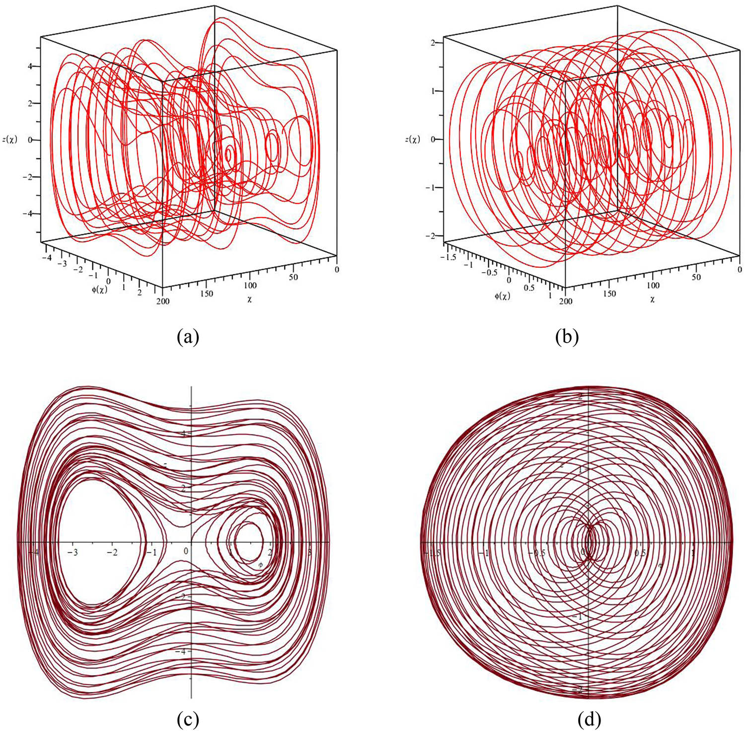
The phase portraits of Eq. (3.3). (a) 3D phase portrait with A 0 = 3 5 , A 1 = ‒ 2 , A 2 = 1 2 , A 3 = 1 2 , and ω = 5 4 , (b) 3D phase portrait with A 0 = 3 5 , A 1 = 2 , A 2 = 1 2 , A 3 = 1 2 , and ω = 5 4 , (c) 2D phase portrait with A 0 = 3 5 , A 1 = ‒ 2 , A 2 = 1 2 , A 3 = 1 2 , and ω = 5 4 , (d) 2D phase portrait with A 0 = 3 5 , A 1 = 2 , A 2 = 1 2 , A 3 = 1 2 , and ω = 5 4 .

$Figure 3 The Lyapunov exponent diagram of Eq. (3.3) with A 0 = 3 5 {A}_{0}=\frac{3}{5} , A 1 = ‒ 2 {A}_{1}=‒2 , A 2 = 1 2 {A}_{2}=\frac{1}{2} , A 3 = 1 2 {A}_{3}=\frac{1}{2} , and ω = 5 4 \omega =\frac{5}{4} .$

Figure 3

The Lyapunov exponent diagram of Eq. (3.3) with A 0 = 3 5 , A 1 = ‒ 2 , A 2 = 1 2 , A 3 = 1 2 , and ω = 5 4 .

Remark 3.1

Through the 3D and 2D phase portraits of system Eq. (3.3) in Figure 2, we can see that Figure 2(a) and (c) are chaotic behaviors. However, Figure 2(b) and (d) exhibit a quasi-periodic behavior.

Remark 3.2

Through the Lyapunov exponent diagram of system Eq. (3.3) in Figure 3, we can see that among the three variables, the exponent of variable ϕ tends to be 0.128 > 0 , the exponent of variable z tends to be 0, and the exponent of variable y tends to be − 0.128 . Since one of the variables has a Lyapunov exponent diagram greater than zero, we can explain that system Eq. (3.3) is a chaotic system.

4 Traveling wave solutions of Eq. (1.1)

First, we will write Eqs (2.5) and (2.6) in integral form as follows:

(4.1) ± ( η − η 0 ) = ∫ d ω κ ( ω 4 + p ω 2 + q ω + r ) ,

where η 0 is the integral constant and κ = ± 1 .

According to the complete discriminant system of polynomial [61] F ( ω ) = ω 4 + p ω 2 + q ω + r , the classification of all solutions of Eq. (4.1) can be obtained. There are nine cases in which the traveling wave solutions of Eq. (1.1) can be obtained.

Case 1. Suppose that G 2 < 0 , G 3 = 0 , G 4 = 0 , F ( ω ) = [ ( ω − a ) 2 + b 2 ] 2 , where a and b are real numbers and b > 0 . Let κ = 1 , it can be obtained from Eq. (4.1)

(4.2) η − η 0 = ∫ d ω ( ω − a ) 2 + b 2 = 1 b arctan ω − a b ,

where η 0 is the integral constant. So, the solution to Eq. (2.5) is

(4.3) ω = b tan [ b ( η − η 0 ) ] + a ,

it is a periodic solution of a trigonometric function. So, the solution of Eq. (1.1) is

(4.4) φ 1 = b tan b − 1 2 5 2 λ 6 − ( 1 − f ) C 3 − f σ 3 D 3 1 4 1 ϱ ξ ϱ − V 1 ϱ τ ϱ − η 0 + a × − 1 2 5 2 λ 6 − ( 1 − f ) C 3 − f σ 3 D 3 − 1 4 − 3 2 λ 4 − ( 1 − f ) C 2 − f σ 2 D 2 3 5 2 λ 6 − ( 1 − f ) C 3 − f σ 3 D 3 .

Case 2. Suppose that G 2 = 0 , G 3 = 0 , G 4 = 0 , and F ( ω ) = ω 4 . Let κ = 1 , it can be obtained from Eq. (4.1)

(4.5) η − η 0 = ∫ d ω ω 2 = − ω − 1 ,

where η 0 is the integral constant. So, the solution to Eq. (2.5) is

(4.6) ω = − ( η − η 0 ) − 1 ,

it is a rational number solution. So, the solution of Eq. (1.1) is

(4.7) φ 2 = − 1 2 5 2 λ 6 − ( 1 − f ) C 3 − f σ 3 D 3 1 4 × 1 ϱ ξ ϱ − V 1 ϱ τ ϱ − η 0 − 1 × − 1 2 5 2 λ 6 − ( 1 − f ) C 3 − f σ 3 D 3 − 1 4 − 3 2 λ 4 − ( 1 − f ) C 2 − f σ 2 D 2 3 5 2 λ 6 − ( 1 − f ) C 3 − f σ 3 D 3 .

Case 3. Suppose that G 2 > 0 , G 3 = 0 , G 4 = 0 , E 2 > 0 , F ( ω ) = ( ω − a ) 2 ( ω − b ) 2 , where a , b are real numbers and a > b . If κ = 1 , it can be obtained from Eq. (4.1)

(4.8) ± ( η − η 0 ) = ∫ d ω ( ω − a ) ( ω − b ) = 1 a − b ln ω − a ω − b ,

where η 0 is the integral constant.

(i) If ω > a or ω < b , the solution to Eq. (2.5) is

(4.9) ω = b − a e ( a − b ) ( η − η 0 ) − 1 + b = b − a 2 × coth ( a − b ) ( η − η 0 ) 2 − 1 + b .

References

[1] Karakoc SBG, Saha A, Sucu DY. A collocation algorithm based on septic B-splines and bifurcation of traveling waves for Sawada-Kotera equation. Math Comput Simulat. 2023;203:12–6. 10.1016/j.matcom.2022.06.020Search in Google Scholar
[2] Karakoc SBG, Saha A, Bhowmik SK, Sucu DY Numerical and dynamical behaviors of nonlinear traveling wave solutions of the Kudryashov-Sinelshchikov equation. Wave Motion. 2023;118:103121. 10.1016/j.wavemoti.2023.103121Search in Google Scholar
[3] Karakoc SBG, Ali KK, Sucu DY. A new perspective for analytical and numerical soliton solutions of the Kaup-Kupershmidt and Ito equations. J Comput Appl Math. 2023;421:114850. 10.1016/j.cam.2022.114850Search in Google Scholar
[4] Wang J, Li Z. A dynamical analysis and new traveling wave solution of the fractional coupled Konopelchenko-Dubrovsky model. Fractal Fract. 2024;8:341. 10.3390/fractalfract8060341Search in Google Scholar
[5] Wu J, Yang Z. Global existence and boundedness of chemotaxis-fluid equations to the coupled Solow-Swan model. AIMS Math. 2023;8:17914–29. 10.3934/math.2023912Search in Google Scholar
[6] Sivasundaram S, Kumar A, Singh RK. On the complex properties to the first equation of the Kadomtsev-Petviashvili hierarchy. Int J Math Comput Eng. 2024;2(1):71–14. 10.2478/ijmce-2024-0006Search in Google Scholar
[7] Li Z, Hussain E. Qualitative analysis and optical solitons for the (1+1)-dimensional Biswas-Milovic equation with parabolic law and nonlocal nonlinearity. Results Phys. 2024;56:107304. 10.1016/j.rinp.2023.107304Search in Google Scholar
[8] Gu MS, Peng C, Li Z. Traveling wave solution of (3+1)-dimensional negative-order KdV-Calogero-Bogoyavlenskii-Schiff equation. AIMS Math. 2024;9(3):6699–10. 10.3934/math.2024326Search in Google Scholar
[9] Liu CY, Li Z. The dynamical behavior analysis and the traveling wave solutions of the stochastic Sasa-Satsuma equation. Qual Theor Dyn Syst. 2024;23:157. 10.1007/s12346-024-01022-ySearch in Google Scholar
[10] Mulimani M, Srinivasa K. A novel approach for Benjamin-Bona-Mahony equation via ultraspherical wavelets collocation method. Int J Math Comput Eng. 2024;2(2):39–14. 10.2478/ijmce-2024-0014Search in Google Scholar
[11] Kawashima S, Matsumura A. Asymptotic stability of traveling wave solutions of systems for one-dimensional gas motion. Commun Math Phys. 1985;101:97–31. 10.1007/BF01212358Search in Google Scholar
[12] Ehrnström M, Kalisch H. Traveling waves for the Whitham equation. Differ Integral Equ. 2009;22:1193–18. 10.57262/die/1356019412Search in Google Scholar
[13] Akers BF, Gao W. Wilton ripples in weakly nonlinear model equations. Commun Math Sci. 2012;10:1015–10. 10.4310/CMS.2012.v10.n3.a15Search in Google Scholar
[14] Hoefer MA, Smyth NF, Sprenger P. Modulation theory solution for nonlinearly resonant, fifth-order Korteweg-de Vries, nonclassical, traveling dispersive shock waves. Stud Appl Math. 2019;142(3):219–22. 10.1111/sapm.12246Search in Google Scholar
[15] Wang B, Zhang Y. Traveling wave solutions for a class of reaction-diffusion system. Bound Value Probl. 2021;2021:33. 10.1186/s13661-021-01508-7Search in Google Scholar
[16] Bilal M, Haris H, Waheed A, Faheem M. The analysis of exact solitons solutions in monomode optical fibers to the generalized nonlinear Schrödinger system by the compatible techniques. Int J Math Comput Eng. 2023;1(2):79–22. 10.2478/ijmce-2023-0012Search in Google Scholar
[17] Mahmud AA, Tanriverdi T, Muhamad KA. Exact traveling wave solutions for (2+1)-dimensional Konopelchenko-Dubrovsky equation by using the hyperbolic trigonometric functions methods. Int J Math Comput Eng. 2023;1(1):1–14. 10.2478/ijmce-2023-0002Search in Google Scholar
[18] Gasmi B, Ciancio A, Moussa A, Alhakim A, Mati A. New analytical solutions and modulation instability analysis for the nonlinear (1+1)-dimensional Phi-four model. Int J Math Comput Eng. 2023;1(1):1–13. 10.2478/ijmce-2023-0006Search in Google Scholar
[19] Khater MMA. Novel computational simulation of the propagation of pulses in optical fibers regarding the dispersion effect. Int J Mod Phys B. 2023;37(09):2350083. 10.1142/S0217979223500832Search in Google Scholar
[20] Alquran M. Classification of single-wave and bi-wave motion through fourth-order equations generated from the Ito model. Phys Scripta. 2023;98(8):085207. 10.1088/1402-4896/ace1afSearch in Google Scholar
[21] Sprenger P, Bridges TJ, Shearer M. Traveling wave solutions of the Kawahara equation joining distinct periodic waves. J Nonlinear Sci. 2023;33:79. 10.1007/s00332-023-09922-0Search in Google Scholar
[22] El-Nabulsi RA, Anukool W. Higher-order nonlinear dynamical systems and invariant Lagrangians on a Lie group: the case of nonlocal Hunter-Saxton type Peakons. Qual Theor Dyn Syst. 2024;23:161. 10.1007/s12346-024-01018-8Search in Google Scholar
[23] Faridi WA, Tipu GH, Myrzakulova Z, Myrzakulov R, Akinyemi L. Formation of optical soliton wave profiles of Shynaray-IIA equation via two improved techniques:a comparative study. Opt Quant Electron. 2024;56(1):132. 10.1007/s11082-023-05699-4Search in Google Scholar
[24] Houwe A, Abbagari S, Akinyemi L, Saliou Y, Justin M, Doka SY. Modulation instability, bifurcation analysis and solitonic waves in nonlinear optical media with odd-order dispersion. Phys Lett A. 2023;488:129134. 10.1016/j.physleta.2023.129134Search in Google Scholar
[25] Cheng X, Wang L. Fundamental solutions and conservation laws for conformable time fractional partial differential equation. J Comput Appl Math. 2024;437:115434. 10.1016/j.cam.2023.115434Search in Google Scholar
[26] Khater MMA, Alfalqi SH, Alzaidi JF, Attia RA. Plenty of accurate novel solitary wave solutions of the fractional Chaffee-Infante equation. Results Phys. 2023;48:106400. 10.1016/j.rinp.2023.106400Search in Google Scholar
[27] Shi D, Li Z. New optical soliton solutions to the (n+1) dimensional time fractional order Sinh-Gordon equation. Results Phys. 2023;51:106669. 10.1016/j.rinp.2023.106669Search in Google Scholar
[28] Hussain A, Ali H, Zaman F, Abbas N. New closed form solutions of some nonlinear pseudo-parabolic models via a new extended direct algebraic method. Int J Math Comput Eng. 2024;2(1):35–24. 10.2478/ijmce-2024-0004Search in Google Scholar
[29] Vinodbhai CD, Dubey S. Investigation to analytic solutions of modified conformable time-space fractional mixed partial differential equations. Part Differ Equ Appl Math. 2022;5:100294. 10.1016/j.padiff.2022.100294Search in Google Scholar
[30] Shi D, Li Z, Han TY. New traveling solutions, phase portrait and chaotic pattern for the generalized (2+1)-dimensional nonlinear conformable fractional stochastic Schrödinger equations forced by multiplicative Brownian motion. Results Phys. 2023;52:106837. 10.1016/j.rinp.2023.106837Search in Google Scholar
[31] Khater MMA. A hybrid analytical and numerical analysis of ultra-short pulse phase shifts. Chaos Soliton Fract. 2023;169:113232. 10.1016/j.chaos.2023.113232Search in Google Scholar
[32] Kumar A, Kumar S. Dynamic nature of analytical soliton solutions of the (1+1)-dimensional Mikhailov-Novikov-Wang equation using the unified approach. Int J Math Comput Eng. 2023;1(2):217–12. 10.2478/ijmce-2023-0018Search in Google Scholar
[33] Rezazadeh H, Seadawy AR, Eslami M, Mirzazadeh M. Generalized solitary wave solutions to the time fractional generalized Hirota-Satsuma coupled KdV via new definition for wave transformation. J Ocean Eng Sci. 2019;4(2):77–8. 10.1016/j.joes.2019.01.002Search in Google Scholar
[34] Ali KK, Karakoc SBG, Rezazadeh H. Optical soliton solutions of the fractional perturbed nonlinear Schrodinger equation. TWMS J Appl Eng Math. 2020;10(4):930–10. Search in Google Scholar
[35] Yao S, Rasool T, Hussain R, Rezazadeh H, Inc M. Exact soliton solutions of conformable fractional coupled Burgeras equation using hyperbolic funtion approach. Results Phys. 2021;30:104776. 10.1016/j.rinp.2021.104776Search in Google Scholar
[36] Darvishi MT, Najafi M, Wazwaz AM. Conformable space-time fractional nonlinear (1+1)-dimensional Schrödinger-type models and their traveling wave solutions. Chaos Soliton Fract. 2021;150:111187. 10.1016/j.chaos.2021.111187Search in Google Scholar
[37] Seadawy AR, Ali A, Raddadi MH. Exact and solitary wave solutions of conformable time fractional clannish random walkeras parabolic and Ablowitz-Kaup-Newell-Segur equations via modified mathematical methods. Results Phys. 2021;26:104374. 10.1016/j.rinp.2021.104374Search in Google Scholar
[38] Ameen I, Elboree MK, Taie ROA. Traveling wave solutions to the nonlinear space-time fractional extended KdV equation via efficient analytical approaches. Alex Eng J. 2023;82:468–16. 10.1016/j.aej.2023.10.022Search in Google Scholar
[39] Ali HMS, Habib MA, Miah MM, Miah MM, Akbar MA. Diverse solitary wave solutions of fractional order Hirota-Satsuma coupled KdV system using two expansion methods. Alex Eng J. 2023;66:1001–14. 10.1016/j.aej.2022.12.021Search in Google Scholar
[40] Alquran M, Ali M, Gharaibeh F, Qureshi S. Novel investigations of dual-wave solutions to the Kadomtsev-Petviashvili model involving second-order temporal and spatial-temporal dispersion terms. Part Differ Equ Appl Math. 2023;8:100543. 10.1016/j.padiff.2023.100543Search in Google Scholar
[41] Akinyemi L, Houwe A, Abbagari S, Wazwaz AM, Alshehri HM, Osman MS. Effects of the higher-order dispersion on solitary waves and modulation instability in a monomode fiber. Optik. 2023;288:171202. 10.1016/j.ijleo.2023.171202Search in Google Scholar
[42] Mirzazadeh M, Akbulut A, Taşcan F, Akinyemi L. A novel integration approach to study the perturbed Biswas-Milovic equation with Kudryashovas law of refractive index. Optik. 2022;252:168529. 10.1016/j.ijleo.2021.168529Search in Google Scholar
[43] Debina K, Rezazadehb H, Ullahc N, et al. New soliton wave solutions of a (2+1)-dimensional Sawada-Kotera equation. J Ocean Eng Sci. 2023;8(5):527–6. 10.1016/j.joes.2022.03.007Search in Google Scholar
[44] Nasreen N, Younas U, Lu D, Zhang Z, Rezazadeh H, Hosseinzadeh MA. Propagation of solitary and periodic waves to conformable ion sound and Langmuir waves dynamical system. Opt Quant Electron. 2023;55:868. 10.1007/s11082-023-05102-2Search in Google Scholar
[45] El-Nabulsi RA. The fractional Boltzmann transport equation. Comput Math Appl. 2011;62 (3):1568–8. 10.1016/j.camwa.2011.03.040Search in Google Scholar
[46] El-Nabulsi RA. Nonlocal-in-time kinetic energy in nonconservative fractional systems, disordered dynamics, jerk and snap and oscillatory motions in the rotating fluid tube. Int J Non-Lin Mech. 2017;93:65–17. 10.1016/j.ijnonlinmec.2017.04.010Search in Google Scholar
[47] Bouaouid M, Hilal K, Melliani S. Nonlocal conformable fractional Cauchy problem with sectorial operator. Indian J Pure and Ap Mat. 2019;50:999–12. 10.1007/s13226-019-0369-9Search in Google Scholar
[48] Khater MMA. Abundant and accurate computational wave structures of the nonlinear fractional biological population model. Int J Mod Phys B. 2023;37(18):2350176. 10.1142/S021797922350176XSearch in Google Scholar
[49] Alquran M. The amazing fractional Maclaurin series for solving different types of fractional mathematical problems that arise in physics and engineering. Part Differ Equ Appl Math. 2023;7:100506. 10.1016/j.padiff.2023.100506Search in Google Scholar
[50] Nasreen N, Lu D, Zhang Z, Akgül A, Younas U, Nasreen S, et al. Propagation of optical pulses in fiber optics modelled by coupled space-time fractional dynamical system. Alex Eng J. 2023;73:173–15. 10.1016/j.aej.2023.04.046Search in Google Scholar
[51] Han TY, Jiang YY. Bifurcation, chaotic pattern and traveling wave solutions for the fractional Bogoyavlenskii equation with multiplicative noise. Phys Scripta. 2024;99:035207. 10.1088/1402-4896/ad21caSearch in Google Scholar
[52] Ray SS. Numerical solutions and solitary wave solutions of fractional KDV equations using modified fractional reduced differential transform method. Comp Math Math Phys. 2013;53:1870–12. 10.1134/S0965542513120142Search in Google Scholar
[53] Zafar A, Rezazadeh H, Bekir A, Malik A. Exact solutions of (3+1)-dimensional fractional mKdV equations in conformable form via exp (ϕ(τ)) expansion method. Sn Appl Sci. 2019;1:1436. 10.1007/s42452-019-1424-1Search in Google Scholar
[54] Karakoc SBG, Saha A, Sucu D. A novel implementation of Petrov-Galerkin method to shallow water solitary wave pattern and superperiodic traveling wave and its multistability:Generalized Korteweg-de Vries equation. Chinese J Phys. 2020;68:605–13. 10.1016/j.cjph.2020.10.010Search in Google Scholar
[55] An T, Liu S. Inverted ternary OPD based on PEIE. Opt Quant Electron 2021;53:669. 10.1007/s11082-021-03344-6Search in Google Scholar
[56] Arefin MA, Sadiya U, Inc M, Uddin MH. Adequate soliton solutions to the space-time fractional telegraph equation and modified third-order KdV equation through a reliable technique. Opt Quant Electron 2022;54:309. 10.1007/s11082-022-03640-9Search in Google Scholar
[57] El-Nabulsi RA. Emergence of lump-like solitonic waves in Heimburg-Jackson biomembranes and nerves fractal model. J R Soc Interface. 2022;19:20220079. 10.1098/rsif.2022.0079Search in Google Scholar PubMed PubMed Central
[58] Eslami M. Optical solutions to a conformable fractional extended KdV model equation. Part Differ Equ Appl Math. 2023;8:100562. 10.1016/j.padiff.2023.100562Search in Google Scholar
[59] Li Z, Han TY. Bifurcation and exact solutions for the (2+1)-dimensional conformable time-fractional Zoomeron equation. Adv Differ Equ-ny. 2020;2020:656. 10.1186/s13662-020-03119-5Search in Google Scholar
[60] Li J, Dai H. On the study of singular nonlinear traveling wave equations: dynamical system approach. Beijing: Science Press; 2007. 10.1142/S0218127407019858Search in Google Scholar
[61] Liu CS. Applications of complete discrimination system for polynomial for classifications of traveling wave solutions to nonlinear differential equations. Comput Phys Commun. 2010;181:317–8. 10.1016/j.cpc.2009.10.006Search in Google Scholar
© 2024 the author(s), published by De Gruyter
This work is licensed under the Creative Commons Attribution 4.0 International License.
Articles in the same Issue
- Regular Articles
- Numerical study of flow and heat transfer in the channel of panel-type radiator with semi-detached inclined trapezoidal wing vortex generators
- Homogeneous–heterogeneous reactions in the colloidal investigation of Casson fluid
- High-speed mid-infrared Mach–Zehnder electro-optical modulators in lithium niobate thin film on sapphire
- Numerical analysis of dengue transmission model using Caputo–Fabrizio fractional derivative
- Mononuclear nanofluids undergoing convective heating across a stretching sheet and undergoing MHD flow in three dimensions: Potential industrial applications
- Heat transfer characteristics of cobalt ferrite nanoparticles scattered in sodium alginate-based non-Newtonian nanofluid over a stretching/shrinking horizontal plane surface
- The electrically conducting water-based nanofluid flow containing titanium and aluminum alloys over a rotating disk surface with nonlinear thermal radiation: A numerical analysis
- Growth, characterization, and anti-bacterial activity of l-methionine supplemented with sulphamic acid single crystals
- A numerical analysis of the blood-based Casson hybrid nanofluid flow past a convectively heated surface embedded in a porous medium
- Optoelectronic–thermomagnetic effect of a microelongated non-local rotating semiconductor heated by pulsed laser with varying thermal conductivity
- Thermal proficiency of magnetized and radiative cross-ternary hybrid nanofluid flow induced by a vertical cylinder
- Enhanced heat transfer and fluid motion in 3D nanofluid with anisotropic slip and magnetic field
- Numerical analysis of thermophoretic particle deposition on 3D Casson nanofluid: Artificial neural networks-based Levenberg–Marquardt algorithm
- Analyzing fuzzy fractional Degasperis–Procesi and Camassa–Holm equations with the Atangana–Baleanu operator
- Bayesian estimation of equipment reliability with normal-type life distribution based on multiple batch tests
- Chaotic control problem of BEC system based on Hartree–Fock mean field theory
- Optimized framework numerical solution for swirling hybrid nanofluid flow with silver/gold nanoparticles on a stretching cylinder with heat source/sink and reactive agents
- Stability analysis and numerical results for some schemes discretising 2D nonconstant coefficient advection–diffusion equations
- Convective flow of a magnetohydrodynamic second-grade fluid past a stretching surface with Cattaneo–Christov heat and mass flux model
- Analysis of the heat transfer enhancement in water-based micropolar hybrid nanofluid flow over a vertical flat surface
- Microscopic seepage simulation of gas and water in shale pores and slits based on VOF
- Model of conversion of flow from confined to unconfined aquifers with stochastic approach
- Study of fractional variable-order lymphatic filariasis infection model
- Soliton, quasi-soliton, and their interaction solutions of a nonlinear (2 + 1)-dimensional ZK–mZK–BBM equation for gravity waves
- Application of conserved quantities using the formal Lagrangian of a nonlinear integro partial differential equation through optimal system of one-dimensional subalgebras in physics and engineering
- Nonlinear fractional-order differential equations: New closed-form traveling-wave solutions
- Sixth-kind Chebyshev polynomials technique to numerically treat the dissipative viscoelastic fluid flow in the rheology of Cattaneo–Christov model
- Some transforms, Riemann–Liouville fractional operators, and applications of newly extended M–L (p, s, k) function
- Magnetohydrodynamic water-based hybrid nanofluid flow comprising diamond and copper nanoparticles on a stretching sheet with slips constraints
- Super-resolution reconstruction method of the optical synthetic aperture image using generative adversarial network
- A two-stage framework for predicting the remaining useful life of bearings
- Influence of variable fluid properties on mixed convective Darcy–Forchheimer flow relation over a surface with Soret and Dufour spectacle
- Inclined surface mixed convection flow of viscous fluid with porous medium and Soret effects
- Exact solutions to vorticity of the fractional nonuniform Poiseuille flows
- In silico modified UV spectrophotometric approaches to resolve overlapped spectra for quality control of rosuvastatin and teneligliptin formulation
- Numerical simulations for fractional Hirota–Satsuma coupled Korteweg–de Vries systems
- Substituent effect on the electronic and optical properties of newly designed pyrrole derivatives using density functional theory
- A comparative analysis of shielding effectiveness in glass and concrete containers
- Numerical analysis of the MHD Williamson nanofluid flow over a nonlinear stretching sheet through a Darcy porous medium: Modeling and simulation
- Analytical and numerical investigation for viscoelastic fluid with heat transfer analysis during rollover-web coating phenomena
- Influence of variable viscosity on existing sheet thickness in the calendering of non-isothermal viscoelastic materials
- Analysis of nonlinear fractional-order Fisher equation using two reliable techniques
- Comparison of plan quality and robustness using VMAT and IMRT for breast cancer
- Radiative nanofluid flow over a slender stretching Riga plate under the impact of exponential heat source/sink
- Numerical investigation of acoustic streaming vortices in cylindrical tube arrays
- Numerical study of blood-based MHD tangent hyperbolic hybrid nanofluid flow over a permeable stretching sheet with variable thermal conductivity and cross-diffusion
- Fractional view analytical analysis of generalized regularized long wave equation
- Dynamic simulation of non-Newtonian boundary layer flow: An enhanced exponential time integrator approach with spatially and temporally variable heat sources
- Inclined magnetized infinite shear rate viscosity of non-Newtonian tetra hybrid nanofluid in stenosed artery with non-uniform heat sink/source
- Estimation of monotone α-quantile of past lifetime function with application
- Numerical simulation for the slip impacts on the radiative nanofluid flow over a stretched surface with nonuniform heat generation and viscous dissipation
- Study of fractional telegraph equation via Shehu homotopy perturbation method
- An investigation into the impact of thermal radiation and chemical reactions on the flow through porous media of a Casson hybrid nanofluid including unstable mixed convection with stretched sheet in the presence of thermophoresis and Brownian motion
- Establishing breather and N-soliton solutions for conformable Klein–Gordon equation
- An electro-optic half subtractor from a silicon-based hybrid surface plasmon polariton waveguide
- CFD analysis of particle shape and Reynolds number on heat transfer characteristics of nanofluid in heated tube
- Abundant exact traveling wave solutions and modulation instability analysis to the generalized Hirota–Satsuma–Ito equation
- A short report on a probability-based interpretation of quantum mechanics
- Study on cavitation and pulsation characteristics of a novel rotor-radial groove hydrodynamic cavitation reactor
- Optimizing heat transport in a permeable cavity with an isothermal solid block: Influence of nanoparticles volume fraction and wall velocity ratio
- Linear instability of the vertical throughflow in a porous layer saturated by a power-law fluid with variable gravity effect
- Thermal analysis of generalized Cattaneo–Christov theories in Burgers nanofluid in the presence of thermo-diffusion effects and variable thermal conductivity
- A new benchmark for camouflaged object detection: RGB-D camouflaged object detection dataset
- Effect of electron temperature and concentration on production of hydroxyl radical and nitric oxide in atmospheric pressure low-temperature helium plasma jet: Swarm analysis and global model investigation
- Double diffusion convection of Maxwell–Cattaneo fluids in a vertical slot
- Thermal analysis of extended surfaces using deep neural networks
- Steady-state thermodynamic process in multilayered heterogeneous cylinder
- Multiresponse optimisation and process capability analysis of chemical vapour jet machining for the acrylonitrile butadiene styrene polymer: Unveiling the morphology
- Modeling monkeypox virus transmission: Stability analysis and comparison of analytical techniques
- Fourier spectral method for the fractional-in-space coupled Whitham–Broer–Kaup equations on unbounded domain