Numerical simulations for fractional Hirota–Satsuma coupled Korteweg–de Vries systems
-
 ,
,

Abstract
In this investigation, the fractional Hirota–Satsuma coupled Korteweg–de Vries (KdV) problem is solved using two modern semi-analytic techniques known as the Aboodh residual power series method (ARPSM) and Aboodh transform iteration method (ATIM). The two suggested approaches are briefly explained, along with how to use them to solve the fractional Hirota–Satsuma coupled KdV problem. Some analytical approximate solutions for the current problem are derived using the proposed techniques until the second-order approximation. To ensure high accuracy of the derived approximation, they are analyzed numerically and graphically and compared with the exact solutions of the integer cases. The offered techniques demonstrate more accuracy in their outcomes compared to other alternatives. The numerical results show that ARPSM and ATIM are highly accurate, practical, and beneficial for solving nonlinear equation systems. The current results are expected to help many physics researchers in modeling their different physical problems, especially those interested in plasma physics.
1 Introduction
Fractional differential equations (FDEs) have become more and more common in various fields of research over the past few decades. They can better explain numerous critical phenomena in acoustics, electromagnetics, electrochemistry, viscoelasticity, cosmology, and materials science. As such, the solution of the FDEs has received a great deal of interest. Nonlinear processes significantly influence physics, applied mathematics, and engineering-related problems. Nonlinear differential equations are used to describe many of these physical phenomena. Differential equations continue to be a significant problem in mathematics and physics that calls for creative solutions that can be either exact or approximative. Most recently developed linear and nonlinear equations have not had a precise analytical solution; hence, numerical methods have been used to solve them [1–5].
Compared to linear differential equations, nonlinear partial differential equations (PDEs) are more challenging to solve [6–8]. Therefore, it might only sometimes be possible to find these equations’ analytical solutions. Here, we employ semi-analytical techniques that yield series solutions [9–11]. These types of approaches look for answers in the form of sequences. The foundation of semi-analytical approaches is determining the other terms in the series, given the problem’s beginning circumstances. This is where the idea of series convergence comes into play. Thus, a convergence study of these techniques is required. Since this convergence analysis can be performed theoretically, the absolute error between the numerical and analytical solutions may be used to determine if the series solution is convergent. A perfect convergence may be obtained in semi-analytic approaches with only a few terms of the series, although more terms may be required in some instances. In other words, a higher sequence of terms leads to a greater convergence of the analytical solution [12–15]. Guo and Hu presented a practical predefined-time stabilization method for high-order systems with unknown disturbances, using a time base generator [16]. Chen et al. proposed a finite-time velocity-free rendezvous control strategy for multiple autonomous underwater vehicle systems with intermittent communication [17]. Yang and Kai investigated dynamical properties and chaotic behaviors in nonlinear coupled Schrödinger equations, particularly in fiber Bragg gratings [18]. Kai and Yin analyzed Gaussian traveling wave solutions in a Schrodinger equation with logarithmic nonlinearity [19]. Zhou et al. introduced an iterative threshold algorithm for log-sum regularization in sparse problems [20]. Finally, Li et al. presented an improved fractional Tikhonov regularization method for moving force identification, providing advancements in structural engineering applications [21].
Research on shallow water equations is a fascinating and fruitful area. Shallow water theory is helpful in a variety of application domains, for example, river floods, building breakwaters, physical oceanography, coastal engineering, tsunami forecasting, and dam break problems. Shallow flow equations are frequently employed in flood analysis since it is well known that they effectively estimate the impacts of floods spreading over extensive terrain. The analytical solutions to these equations can also be used to obtain a good idea of the height of the waves along the coast and how their speed distribution changes over time on a sloping beach and in coastal areas. Shallow water wave equations express the height and velocity of the current flowing through the channels of a rainwater drainage network. They are also employed in the computation of ocean flows and vorticity [22,23]. Consider the following fractional-order Hirota–Satsuma coupled Korteweg–de Vries (KdV):
with the following initial conditions (ICs):
where
Several authors [24–30] have examined System 1 with constant coefficients. In the study by Kaya [24], the isolated wave solutions are derived using the decomposition method. In the study by Yong et al. [25], multiple explicit solutions are obtained using the homogeneous method. In the study by Yao et al. [26], the traveling wave solutions are derived using the Ritt–Wu method. In the study by Xu et al. [28], the traveling wave solutions (TWSs) are obtained using the maple package TRWS, and finally, in the studies by Liu et al. [29] and Qing-You et al. [30], the periodic wave solutions are given.
A significant class of nonlinear evolution equations, KdV-type equations, have many uses in engineering and physical research. Acoustic waves are a product of these equations in plasma physics [31–34], and they describe a long wave in both shallow and deep oceans in geophysical fluid dynamics [35]. Cluster physics, super-deformed nuclei, fission, thin films, radar, rheology [36,37], optical-fiber communications [38], and superconductors [39] are all areas where they are present. Because they assume constant coefficients, the physical circumstances that give birth to the KdV equations are often idealized. For this reason, several types of KdV equations involving variable coefficients [40–44] have received a lot of focus as of late in the search for accurate solutions. Two long waves’ interaction is described by a set of linked KdV equations with variable coefficients [45,46], which has been examined recently by some others.
In 2013, Arqub introduced a semi-analytical methodology called the residual power series method (RPSM) [47]. This method combines Taylor’s series with the residual error function. As its first venture into the domain of fuzzy differential equation resolution, this novel approach proved its adaptability by effectively solving both linear and nonlinear differential equations. To solve complicated DEs using power series methods, Mukhtar et al. [48] developed a unique set of RPSM algorithms. Then, separate equations with modifications made may be solved. Finally, the inverse Aboodh transform (AT) is used to solve the original equation. This new strategy uses homotopy perturbation methods with the Sumudu transform. We solve linear and nonlinear PDEs using the unique power series expansion approach, which does not need linearization, perturbation, or discretization. In RPSM, the calculation of fractional derivatives requires several solution iterations, but here, the computations of coefficients are much more straightforward. Using a quick convergence series, the suggested approach can provide a close approximate solution.
The most significant mathematical accomplishment of the twentieth century was the Aboodh transform iterative approach (ATIM) for fractional PDEs. Regular methods of solving PDEs with fractional derivatives are infamously tricky because of the computing complexity and non-convergence of these problems. Our unique technology goes beyond these restrictions by reducing processing effort, enhancing accuracy, and continuously improving approximation solutions. Iterations tailored to fractional derivatives have improved the solutions to complex mathematical and physical problems [49–51]. Complex fractional PDE-governed systems may now be used to study challenging engineering, applied mathematics, and physics problems.
The Aboodh residual power series method (ARPSM) and ATIM are two of the most basic strategies for solving FDEs [52,53]. In addition to giving analytical answers in symbolic terms that can be accessed immediately, these approaches also provide numeric approximate results to linear and nonlinear differential equations that do not need discretization or linearization. Finding solutions to fractional order Hirota–Satsuma coupled KdV using two different approaches, ARPSM and ATIM, is the main objective of this study. These two methods have been used together to resolve many nonlinear fractional differential problems.
2 Fundamental definitions
Definition 2.1
Let exponentially ordered function
The inverse AT is expressed in the following way:
where
Lemma 2.2
Consider the following functions:
Definition 2.3
The fractional Caputo derivative of a function
where
Definition 2.4
We may write the power series as [58]:
where
Lemma 2.5
The AT is represented as
where
Proof
Now, we use the induction approach to verify Eq. (3). The following result is obtained when
Lemma 2.2, specifically Part (4) proves that the equation is true for
We obtain the following by taking into account the left-hand side (L.H.S.) of Eq. (4):
A specific way to write Eq. (5) is as follows:
Let
Therefore, Eq. (6) changes to:
With the help of the fractional derivative of the Caputo type.
The formula for the Riemann–Liouville (RL) fractional integral of the AT is given by Eq. (9):
Using the differential property of AT, Eq. (10) is changed to
In light of Eq. (7), we are able to determine
where
Note that Eqs (3) and (12) are compatible with each other. With the assumption that Eq. (3) is valid for
Eq. (3) will be shown to be true for
In Eq. (14), on L.H.S., we obtain
Consider
Eq. (15) gives us
By combining the fractional Caputo derivative with the RL integral formula, Eq. (16) may be expressed as
With the help of Eqs (13) and (17), it is transformed into
Eq. (18) allows us to obtain the subsequent outcome:
This proves that Eq. (3) is valid for
Lemma 2.6
Consider the exponentially ordered function
where
Proof
Performing a fractional order analysis on Taylor’s series, we obtain
By applying the AT on Eq. (20), the following equality is obtained:
These characteristics of the AT allow us to derive
As a result, we obtain (19), a new Taylor’s series in the AT.□
Theorem 2.7
Following are the multiple fractional power series (MFPS) representations of the functions
where
where
Proof
The new version of Taylor’s series provides us
This may be achieved by solving Eq. (21) for
The following equality is the result of taking the limit:
The following result is produced when Lemma 2.5 is combined with Eq. (22):
In addition, Eq. (23) in conjunction with Lemma 2.6 yields the following result:
The result is obtained using the modified Taylor’s series together with
We obtain the result using Lemma 2.6:
Eq. (24) is transformed once again using Lemmas 2.5 and 2.6 with Theorem 2.7:
Applying the same process to the new form of Taylor’s series yields
The final equation is obtained using Lemma 2.6:
In general, we obtain
This concludes the proof.□
Theorem 2.8
A new multiple fractional Taylor’s formula is shown in
Lemma 2.6
with
Theorem 2.7
and is denoted as
Proof
The following assumptions serve as the foundation for the proof:
When Theorem 2.7 is applied, Eq. (25) becomes
Multiply
Applying Lemma 2.5 to Eq. (27) yields
Taking Eq. (28)’s absolute yields
Applying the conditions given in Eq. (29) results in the following conclusion:
Eq. (30) leads to the desired outcome
This establishes the convergence requirement for the new series.□
3 Methodologies
3.1 Implementation of the ARPSM
In order to address our general model, we propose the ARPSM fundamentals.
Step 1: Write the equation in standard form:
Step 2: Eq. (31) may be solved by applying AT on both sides to obtain
Lemma 2.5 will be used to transform Eq. (32):
where
Step 3: To solve Eq. (33), take into consideration the following form:
Step 4: Follow these steps:
The following outcome is achieved using Theorem 2.8:
Step 5: Follow these procedures to obtain
Step 6: ARF of Eq. (33) has to be evaluated separately from the
and
Step 7: In Eq. (34), substitute the expansion form of
Step 8: Multiply
Step 9: Both sides of Eq. (36) are being evaluated with respect to
Step 10: We need to solve the following equation to obtain
where
Step 11: The
Step 12: The
3.1.1 ARPSM for anatomy fractional Hirota–Satsuma coupled KdV
Let us investigate the following fractional Hirota–Satsuma coupled KdV [24–27]:
which support the following exact solutions for the integer cases [27]:
where
For simplicity, during our calculations, we can use
and accordingly, the IC’s for problem (37) can be written in the following manner:
Using Eq. (42) and applying AT on System (37), we obtain
Thus, the term series that is
for
Aboodh residual functions (ARFs) read
where
where
To find the values of the functions
Multiply the resulting equations by
Then, iteratively solve the relations
Finally, the following first few terms are obtained:
(47)and
(48)and so on.
Putting the obtained values of
Applying the inverse AT on system (49) yields
From now on, we use
The convergence of ARPSM can be examined by presenting some numerical examples for the derived approximations. Accordingly, the three approximations (50)–(52) are analyzed numerically and graphically, as illustrated in Tables 1, 2, 3. We also calculated the absolute error of the three approximations compared to the exact solutions for the integer cases, as shown in Tables 1–3 in addition to Figures 1, 2, 3. Figure 1 displays the absolute error of the approximation (50) as compared to the exact solution (39), while Table 1 also showcases the outcomes of the approximation (50) analysis. Figure 2 shows the absolute error of the approximation (51) as compared to the exact solution (40), while Table 2 displays the findings of the analysis of the approximation (51). Moreover, Figure 3 indicates the absolute error of the approximation (52) as compared to the exact solution (41), while Table 3 displays the numerical analysis of the approximation (52) against the fractional parameter. It is clear from the obtained results that there is no difference between the approximate and exact solutions for the integer cases, meaning that there is complete harmony between these solutions, which enhances the accuracy of the deduced approximations and the efficiency of the used method. It is worth noting that we arrived at this result by obtaining a few numbers of terms from the solution series. Thus, the accuracy of these approximations can be increased by deriving a larger number of terms in the solution series. This result confirms the convergence and the efficiency of the ARPSM in analyzing more complicated nonlinear evolution equations.
Approximation (50) is numerically analyzed against the fractional parameter (
|
|
|
|
|
Exact |
|
|---|---|---|---|---|---|
|
|
1.66613 | 1.66628 | 1.6663 | 1.6663 |
|
|
|
1.66274 | 1.66384 | 1.66393 | 1.66393 |
|
|
|
1.63782 | 1.64584 | 1.64654 | 1.64654 |
|
|
|
1.46307 | 1.51779 | 1.52262 | 1.52262 |
|
|
|
0.564653 | 0.791665 | 0.813862 | 0.813862 |
|
| 0 |
|
|
|
|
|
| 1 | 1.02172 | 0.860674 | 0.83945 | 0.83945 |
|
| 2 | 1.5604 | 1.53249 | 1.52806 | 1.52806 |
|
| 3 | 1.65185 | 1.64796 | 1.64732 | 1.64732 |
|
| 4 | 1.66465 | 1.66412 | 1.66404 | 1.66404 |
|
| 5 | 1.66639 | 1.66632 | 1.66631 | 1.66631 |
|
Approximation (51) is numerically analyzed against the fractional parameter (
|
|
|
|
|
Exact |
|
|---|---|---|---|---|---|
|
|
|
|
|
|
|
|
|
|
|
|
|
|
|
|
|
|
|
|
|
|
|
|
|
|
|
|
|
|
|
|
|
|
|
| 0 | 0.178627 | 0.0269694 | 0.01 | 0.00999967 |
|
| 1 | 0.819361 | 0.772638 | 0.765762 | 0.765762 |
|
| 2 | 0.972974 | 0.965873 | 0.964727 | 0.964727 |
|
| 3 | 0.996288 | 0.995312 | 0.995152 | 0.995152 |
|
| 4 | 0.999497 | 0.999364 | 0.999343 | 0.999343 |
|
| 5 | 0.999932 | 0.999914 | 0.999911 | 0.999911 |
|
Approximation (52) is numerically analyzed against the fractional parameter (
|
|
|
|
|
Exact |
|
|---|---|---|---|---|---|
|
|
|
|
|
|
|
|
|
|
|
|
|
|
|
|
|
|
|
|
|
|
|
|
|
|
|
|
|
|
|
|
|
|
|
| 0 | 0.476339 | 0.0719184 | 0.0266667 | 0.0266658 |
|
| 1 | 2.18496 | 2.06037 | 2.04203 | 2.04203 |
|
| 2 | 2.5946 | 2.57566 | 2.57261 | 2.57261 |
|
| 3 | 2.65677 | 2.65417 | 2.65374 | 2.65374 |
|
| 4 | 2.66532 | 2.66497 | 2.66491 | 2.66491 |
|
| 5 | 2.66648 | 2.66644 | 2.66643 | 2.66643 |
|


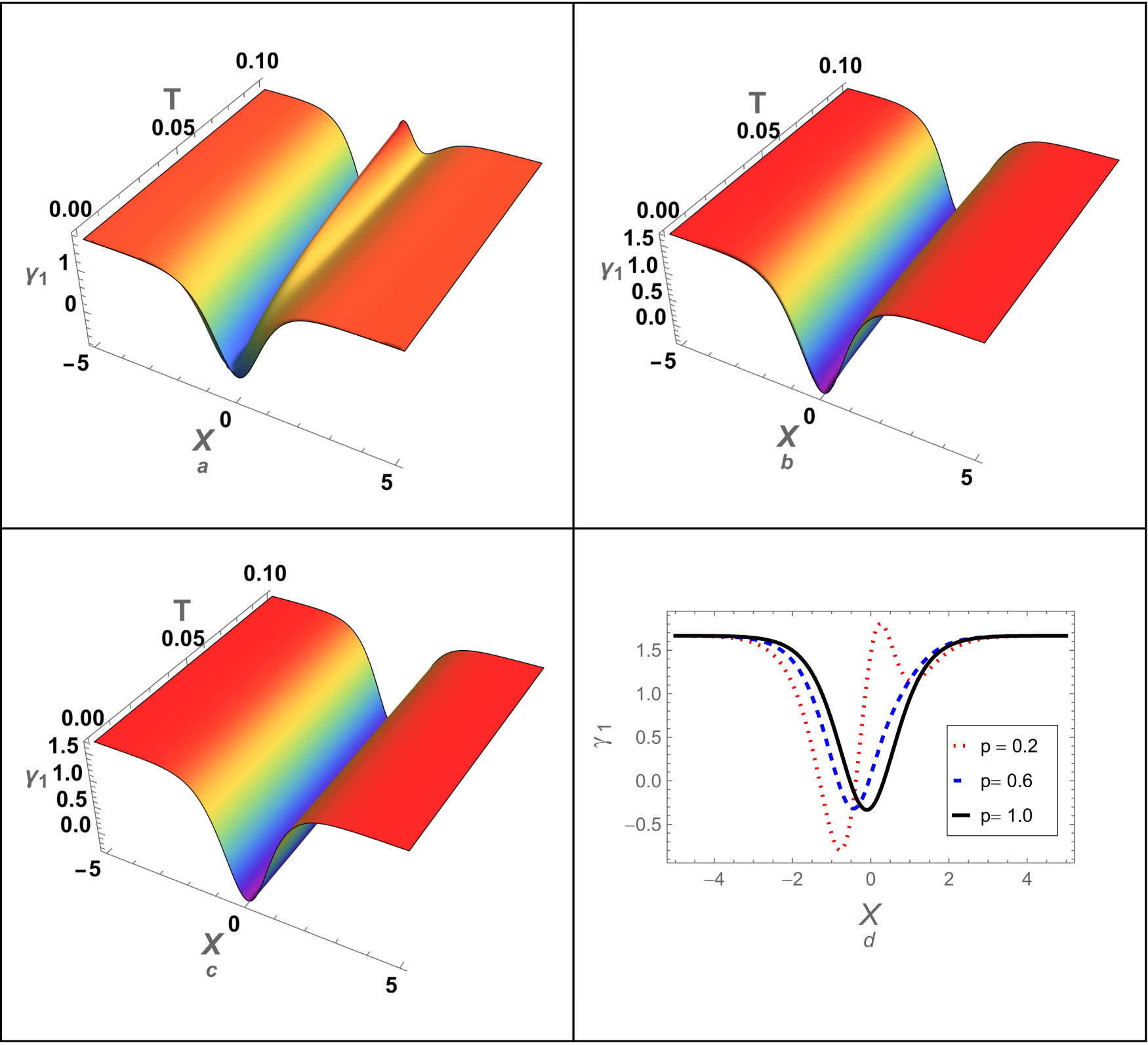
In addition, we studied the effect of the fractional parameter on the profile of both soliton and shock waves described by the derived approximations. It is clear from the analysis results that the fractional parameter significantly affects the profile of both soliton and shock waves, as is evident in Figures 4, 5, 6, for the approximations (50), (51), and (52), respectively.

Approximation (50) is plotted against the fractional parameter

Approximation (51) is plotted against the fractional parameter

Approximation (52) is plotted against the fractional parameter
3.2 ATIM
The general fractional PDE for space and time is given as
with IC’s
where
Then, by applying the inverse AT, the following equation is obtained:
By applying the AT iteratively, the solution in an infinite series is obtained as follows:
where
After inserting Eqs (58) and (57) into Eq. (56), we have
with
Eq. (53) yields the approximate solution for the
3.2.1 ATIM for anatomy fractional Hirota–Satsuma coupled KdV
We apply ATIM to analyze fractional Hirota–Satsuma coupled KdV problem (37) in this section. To avoid repeating the fractional Hirota–Satsuma coupled KdV problem (37) more than once, we only here refer to its number (37) with its ICs (42) as mentioned earlier.
Now, applying the AT to both sides of problem (37) yields the following equations:
where
The following equations are derived by applying the inverse AT to Eq. (62):
The following values for
Applying the RL integral on problem (37) yields the following equivalent form:
where
The terms that derived using the ATIM read:
Zeroth-order approximation
first-order approximation
and second-order approximation
By collecting the values of zeroth-, first-, and second-order approximations given in Eqs (66)–(68), we finally obtain
and
ATIM convergence can be analyzed by providing some numerical examples of the obtained approximations, depending on the variables involved. Consequently, the three approximations (69)–(70) are investigated numerically and graphically, as shown in Tables 4, 5, 6. Also, the absolute errors of the three approximations compared to the exact solutions for the integer cases are estimated as presented in Tables 4–6 and Figures 7, 8, 9. Both Figure 7 and Table 4 show the absolute error between approximation (69) and the exact solution (39) for the integer case. Also, Figure 8 and Table 5 illustrate the absolute error between approximation (70) and the exact solution (40) for the integer case. For the integer case, Figure 9 and Table 6 show a comparison of the approximation (71) and the exact solution (41). The results show that there is no difference between the exact and approximate solutions for integer cases. This means that there is a high level of agreement between these solutions, making the method more accurate and useful. Moreover, the impact of fractional parameter p on the profile of the approximations (69)–(71) is investigated as shown in Figures Figures 10, 11, 12, respectively. We reached this conclusion by extracting a limited number of terms from the solution series. Increasing the number of terms in the solution series can enhance the accuracy of these approximations. This outcome validates the convergence and effectiveness of the ATIM in studying complicated and strong nonlinear evolution equations.
Approximation (69) is numerically analyzed against the fractional parameter (
|
|
|
|
|
Exact |
|
|---|---|---|---|---|---|
|
|
1.66613 | 1.66628 | 1.6663 | 1.6663 |
|
|
|
1.66269 | 1.66383 | 1.66393 | 1.66393 |
|
|
|
1.6374 | 1.64582 | 1.64653 | 1.64654 |
|
|
|
1.4591 | 1.51764 | 1.52259 | 1.52262 | 0.0000253808 |
|
|
0.555815 | 0.7913 | 0.813799 | 0.813862 | 0.0000628624 |
| 0 |
|
|
|
|
0.000200013 |
| 1 | 1.01828 | 0.860328 | 0.839388 | 0.83945 | 0.0000614722 |
| 2 | 1.55938 | 1.53235 | 1.52804 | 1.52806 | 0.000025149 |
| 3 | 1.6515 | 1.64794 | 1.64732 | 1.64732 |
|
| 4 | 1.6646 | 1.66412 | 1.66404 | 1.66404 |
|
| 5 | 1.66639 | 1.66632 | 1.66631 | 1.66631 |
|
Approximation (70) is numerically analyzed against the fractional parameter (
|
|
|
|
|
Exact |
|
|---|---|---|---|---|---|
|
|
|
|
|
1.6663 |
|
|
|
|
|
|
1.66393 |
|
|
|
|
|
|
1.64654 |
|
|
|
|
|
|
1.52262 |
|
|
|
|
|
|
0.813862 | 0.0000294264 |
| 0 | 0.178627 | 0.0269694 | 0.01 |
|
|
| 1 | 0.802208 | 0.772407 | 0.765727 | 0.83945 | 0.0000345442 |
| 2 | 0.971667 | 0.965832 | 0.96472 | 1.52806 |
|
| 3 | 0.996177 | 0.995307 | 0.995151 | 1.64732 |
|
| 4 | 0.999483 | 0.999364 | 0.999342 | 1.66404 |
|
| 5 | 0.99993 | 0.999914 | 0.999911 | 1.66631 |
|
Approximation (71) is numerically analyzed against the fractional parameter (
|
|
|
|
|
Exact |
|
|---|---|---|---|---|---|
|
|
|
|
|
|
|
|
|
|
|
|
|
|
|
|
|
|
|
|
|
|
|
|
|
|
|
0.0000177528 |
|
|
|
|
|
|
0.0000784703 |
| 0 | 0.476339 | 0.0719184 | 0.0266667 | 0.0266658 |
|
| 1 | 2.13922 | 2.05975 | 2.04194 | 2.04203 | 0.0000921178 |
| 2 | 2.59111 | 2.57555 | 2.57259 | 2.57261 | 0.0000185712 |
| 3 | 2.65647 | 2.65415 | 2.65374 | 2.65374 |
|
| 4 | 2.66529 | 2.66497 | 2.66491 | 2.66491 |
|
| 5 | 2.66648 | 2.66644 | 2.66643 | 2.66643 |
|


We also numerically compared all derived approximations using ARPSM and ATIM, as shown in Tables 7, 8, 9. In this comparison, we estimated the absolute errors of all derived approximations using ARPSM compared to the exact solutions for integer cases. We also calculated the absolute errors of all derived approximations using ATIM compared to the exact solutions for integer cases. The comparison results show that both methods exhibit high accuracy, convergence, and stability, but ARPSM-derived approximations are more accurate than ATIM-derived ones.
Absolute error for approximation (50) using ARPSM and approximation (69) using ARIM for the integer case are compared to the exact solution (39) at
|
|
ARPSM | ATIM | Exact |
|
|
|---|---|---|---|---|---|
|
|
1.6663 | 1.6663 | 1.6663 |
|
|
|
|
1.66393 | 1.66393 | 1.66393 |
|
|
|
|
1.64654 | 1.64653 | 1.64654 |
|
|
|
|
1.52262 | 1.52259 | 1.52262 |
|
0.0000253808 |
|
|
0.813862 | 0.813799 | 0.813862 |
|
0.0000628624 |
| 0 |
|
|
|
|
0.000200013 |
| 1 | 0.83945 | 0.839388 | 0.83945 |
|
0.0000614722 |
| 2 | 1.52806 | 1.52804 | 1.52806 |
|
0.000025149 |
| 3 | 1.64732 | 1.64732 | 1.64732 |
|
|
| 4 | 1.66404 | 1.66404 | 1.66404 |
|
|
| 5 | 1.66631 | 1.66631 | 1.66631 |
|
|
Absolute error for approximation (51) using ARPSM and approximation (70) using ARIM for the integer case are compared to the exact solution (40) at
|
|
ARPSM | ATIM | Exact |
|
|
|---|---|---|---|---|---|
|
|
|
|
|
|
|
|
|
|
|
|
|
|
|
|
|
|
|
|
|
|
|
|
|
|
|
|
|
|
|
|
|
|
0.0000294264 |
| 0 | 0.01 | 0.01 | 0.00999967 |
|
|
| 1 | 0.765762 | 0.765727 | 0.765762 |
|
0.0000345442 |
| 2 | 0.964727 | 0.96472 | 0.964727 |
|
|
| 3 | 0.995152 | 0.995151 | 0.995152 |
|
|
| 4 | 0.999343 | 0.999342 | 0.999343 |
|
|
| 5 | 0.999911 | 0.999911 | 0.999911 |
|
|
Absolute error for approximation (52) using ARPSM and approximation (71) using ARIM for the integer case are compared to the exact solution (41) at
|
|
ARPSM | ATIM | Exact |
|
|
|---|---|---|---|---|---|
|
|
|
|
|
|
|
|
|
|
|
|
|
|
|
|
|
|
|
|
|
|
|
|
|
|
|
0.0000177528 |
|
|
|
|
|
|
0.0000784703 |
| 0 | 0.0266667 | 0.0266667 | 0.0266658 |
|
|
| 1 | 2.04203 | 2.04194 | 2.04203 |
|
0.0000921178 |
| 2 | 2.57261 | 2.57259 | 2.57261 |
|
0.0000185712 |
| 3 | 2.65374 | 2.65374 | 2.65374 |
|
|
| 4 | 2.66491 | 2.66491 | 2.66491 |
|
|
| 5 | 2.66643 | 2.66643 | 2.66643 |
|
|
Approximation (69) is plotted against the fractional parameter

Approximation (70) is plotted against the fractional parameter

Approximation (71) is plotted against the fractional parameter
4 Conclusion
In conclusion, this study has delved into the intricate dynamics of the fractional Hirota–Satsuma coupled KdV equation employing innovative methodologies such as ATIM and ARPSM. We have briefly discussed the proposed methods and how they can be applied to analyze strong nonlinear and more complicated evolution equations. By applying these advanced techniques, we have successfully provided enhanced analytical approximations for the two mentioned problems in the framework of the Caputo operator. We have analyzed all derived approximations using both ARPSM and ATIM numerically and graphically and calculated their absolute error compared to the exact solutions for the integer cases. The analysis and comparison results showed the high accuracy, convergence, and stability of all derived approximations, which enhanced the techniques’ high efficiency and ability to analyze the more complicated evolution equations. The importance of ATIM and ARPSM in solving nonlinear fractional equations is highlighted, demonstrating their potential applications in several scientific fields, significantly solving evolution equations describing various nonlinear phenomena in plasmas. This study’s breakthroughs facilitate further research and the use of approaches to solve complicated mathematical problems involving fractional operators, thus contributing to nonlinear dynamics and fractional calculus.
Future work: After proving the proposed methods’ high efficiency and accuracy in analyzing more complicated FDEs, these techniques can be used to analyze various evolution equations, which are used to model many nonlinear phenomena that arise and propagate in different plasma systems. For instance, these techniques can be applied to investigate the fractional shapes of the family of KdV-type equations in their integrable and non-integrable forms [59–61], the family of Kawahara-type equations in their integrable and non-integrable forms [62–64], the family of nonlinear Schrödinger-type equations in their integrable and non-integrable forms [65–67], and so on.
Acknowledgments
The authors express their gratitude to Princess Nourah bint Abdulrahman University Researchers Supporting Project number (PNURSP2024R439), Princess Nourah bint Abdulrahman University, Riyadh, Saudi Arabia. This work was supported by the Deanship of Scientific Research, Vice Presidency for Graduate Studies and Scientific Research, King Faisal University, Saudi Arabia (Grant No. 6101).
-
Funding information: The authors expressed their gratitude to Princess Nourah bint Abdulrahman University Researchers Supporting Project number (PNURSP2024R439), Princess Nourah bint Abdulrahman University, Riyadh, Saudi Arabia. This work was supported by the Deanship of Scientific Research, Vice Presidency for Graduate Studies and Scientific Research, King Faisal University, Saudi Arabia (Grant No. 6101).
-
Author contributions: All authors have accepted responsibility for the entire content of this manuscript and approved its submission.
-
Conflict of interest: The authors state no conflict of interest.
-
Data availability statement: Data sharing is not applicable to this article as no new data were created or analyzed in this study.
References
[1] Tenreiro Machado JA, Silva MF, Barbosa RS, Jesus IS, Reis CM, Marcos MG et al. Some applications of fractional calculus in engineering. Math Problems Eng. 2010;2010:639801. 10.1155/2010/639801Search in Google Scholar
[2] Ionescu C, Lopes A, Copot D, Machado JT, Bates JH. The role of fractional calculus in modeling biological phenomena: A review. Commun Nonlinear Sci Numer Simulat. 2017;51:141–59. 10.1016/j.cnsns.2017.04.001Search in Google Scholar
[3] Munusamy K, Ravichandran C, Nisar KS, Munjam SR. Investigation on continuous dependence and regularity solutions of functional integrodifferential equations. Results Control Optim. 2024;14:100376. 10.1016/j.rico.2024.100376Search in Google Scholar
[4] Nisar KS, Anusha C, Ravichandran C. A non-linear fractional neutral dynamic equations: existence and stability results on time scales. AIMS Mathematics. 2024;9(1):1911–25. 10.3934/math.2024094Search in Google Scholar
[5] Noor S, Alshehry AS, Shafee A, Shah R. Families of propagating soliton solutions for (3+1)-fractional Wazwaz-BenjaminBona-Mahony equation through a novel modification of modified extended direct algebraic method. Phys Scr. 2024;99(4):045230. 10.1088/1402-4896/ad23b0Search in Google Scholar
[6] Meng S, Meng F, Zhang F, Li Q, Zhang Y, Zemouche A. Observer design method for nonlinear generalized systems with nonlinear algebraic constraints with applications. Automatica. 2024;162:111512. https://doi.org/10.1016/j.automatica.2024.111512. Search in Google Scholar
[7] Li B, Guan T, Dai L, Duan G. Distributionally Robust model predictive control with output feedback. IEEE Trans Automatic Control. 2023. 10.1109/TAC.2023.3321375. Search in Google Scholar
[8] Cai X, Tang R, Zhou H, Li Q, Ma S, Wang D, et al. Dynamically controlling terahertz wavefronts with cascaded metasurfaces. Adv Photonics. 2021;3(3):036003. 10.1117/1.AP.3.3.036003. Search in Google Scholar
[9] Yeh C, Zhang C, Shi W, Lo M, Tinkhauser G, Oswal A. Cross-frequency coupling and intelligent neuromodulation. Cyborg Bionic Syst. 2023;4:34. 10.34133/cbsystems.0034. Search in Google Scholar PubMed PubMed Central
[10] He T, Zheng Y, Liang X, Li J, Lin L, Zhao W, et al. A highly energy-efficient body-coupled transceiver employing a power-on-demand amplifier. Cyborg Bionic Syst. 2023;4:30. 10.34133/cbsystems.0030. Search in Google Scholar PubMed PubMed Central
[11] He B, Yin L, Zambrano-Serrano E. Prediction modelling of cold chain logistics demand based on data mining algorithm. Math Problems Eng. 2021;2021:3421478. https://doi.org/10.1155/2021/3421478. Search in Google Scholar
[12] Nisar KS, Alsaeed S, Kaliraj K, Ravichandran C, Albalawi W, Abdel-Aty AH. Existence criteria for fractional differential equations using the topological degree method. AIMS Math. 2023;8(9):21914–28. 10.3934/math.20231117Search in Google Scholar
[13] Noor S, Alotaibi BM, Shah R, Ismaeel SM, El-Tantawy SA. On the solitary waves and nonlinear oscillations to the fractional Schrödinger-KdV equation in the framework of the Caputo operator. Symmetry. 2023;15(8):1616. 10.3390/sym15081616Search in Google Scholar
[14] El-Sayed AMA. On the stochastic fractional calculus operators. J Fract Calculus Appl. 2015;6(1):101–9. Search in Google Scholar
[15] Anastassiou GA. Foundation of stochastic fractional calculus with fractional approximation of stochastic processes. Revista de la Real Academia de Ciencias Exactas, Fisicas y Naturales. Serie A. Matematicas. 2020;114(2):89. 10.1007/s13398-020-00817-3Search in Google Scholar
[16] Guo C, Hu J. Time base generator based practical predefined-time stabilization of high-order systems with unknown disturbance. IEEE Trans Circuits Systems II Express Briefs. 2023;70:2670–4. 10.1109/TCSII.2023.3242856. Search in Google Scholar
[17] Chen B, Hu J, Zhao Y, Ghosh BK. Finite-time velocity-free Rendezvous control of multiple AUV systems with intermittent communication. IEEE Trans Syst Man Cybernetic Syst. 2022;52(10):6618–29. 10.1109/TSMC.2022.3148295. Search in Google Scholar
[18] Yang R, Kai Y. Dynamical properties, modulation instability analysis and chaotic behaviors to the nonlinear coupled Schrödinger equation in fiber Bragg gratings. Modern Phys Lett B. 2023;38(6):2350239. https://doi.org/10.1142/S0217984923502391. Search in Google Scholar
[19] Kai Y, Yin Z. On the Gaussian traveling wave solution to a special kind of Schrödinger equation with logarithmic nonlinearity. Modern Phys Lett B. 2021;36(02):2150543. 10.1142/S0217984921505436. Search in Google Scholar
[20] Zhou X, Liu X, Zhang G, Jia L, Wang X, Zhao Z. An iterative threshold algorithm of log-sum regularization for sparse problem. IEEE Trans Circuits Syst Video Technol. 2023;33(9):4728–40. 10.1109/TCSVT.2023.3247944. Search in Google Scholar
[21] Li M, Wang L, Luo C, Wu H. A new improved fractional Tikhonov regularization method for moving force identification. Structures. 2024;60:105840. https://doi.org/10.1016/j.istruc.2023.105840. Search in Google Scholar
[22] Ablowitz MJ, Kaup DJ, Newell AC, Segur H. The inverse scattering transform-Fourier analysis for nonlinear problems. Studies Appl Math. 1974;53(4):249–315. 10.1002/sapm1974534249Search in Google Scholar
[23] Vitanov NK, Dimitrova ZI, Vitanov KN. Simple equations method (SEsM): Algorithm, connection with Hirota method, inverse scattering transform method, and several other methods. Entropy. 2020;23(1):10. 10.3390/e23010010Search in Google Scholar PubMed PubMed Central
[24] Kaya D. Solitary wave solutions for a generalized Hirota-Satsuma coupled KdV equation. Appl Math Comput. 2004;147(1):69–78. 10.1016/S0096-3003(02)00651-3Search in Google Scholar
[25] Yong C, Zhen-Ya Y, Biao L, Hong-Qing Z. New explicit exact solutions for a generalized Hirota-Satsuma coupled KdV system and a coupled MKdV equation. Chinese Phys. 2003;12(1):1. 10.1088/1009-1963/12/1/301Search in Google Scholar
[26] Yao RX, Li ZB. New exact solutions for three nonlinear evolution equations. Phys Lett A. 2002;297(3–4):196–204. 10.1016/S0375-9601(02)00294-3Search in Google Scholar
[27] Fan Engui Soliton solutions for a generalized Hirota-Satsuma coupled KdV equation and a coupled MKdV equation. Phys Lett A. 2001;282:18–22. 10.1016/S0375-9601(01)00161-XSearch in Google Scholar
[28] Xu GQ, Li ZB, Liu YP. Exact solutions to a large class of nonlinear evolution equations. Chin J Phys. 2003;41(3):232–41. Search in Google Scholar
[29] Liu J, Yang L, Yang K. Jacobi elliptic function solutions of some nonlinear PDEs. Phys Lett A. 2004;325(3–4):268–75. 10.1016/j.physleta.2004.03.063Search in Google Scholar
[30] Qing-You Y, Yu-Feng Z, Xiao-Peng W. New periodic solutions to a generalized Hirota-Satsuma coupled KdV system. Chinese Phys. 2003;12(2):131. 10.1088/1009-1963/12/2/301Search in Google Scholar
[31] El-TantawySA, Wazwaz A-M. Anatomy of modified Korteweg-de Vries equation for studying the modulated envelope structures in non-Maxwellian dusty plasmas: Freak waves and dark soliton collisions. Phy Plasmas. 2018;25:092105. 10.1063/1.5045247Search in Google Scholar
[32] Hong HS, Lee HJ. Korteweg-de Vries equation of ion acoustic surface waves. Phys Plasmas. 1999;6(8):3422–4. 10.1063/1.873599Search in Google Scholar
[33] Hashmi T, Jahangir R, Masood W, Alotaibi BM, Ismaeel SME, El-Tantawy SA. Head-on collision of ion-acoustic (modified) Korteweg de Vries solitons in Saturn’s magnetosphere plasmas with two temperature superthermal electrons. Phys Fluids. 2023;35:103104. 10.1063/5.0171220Search in Google Scholar
[34] Arif K, Ehsan T, Masood W, Asghar S, Alyousef HA, Tag-Eldin E, et al. Quantitative and qualitative analyses of the mKdV equation and modeling nonlinear waves in plasma. Frontiers Phys. 2023;11:194. 10.3389/fphy.2023.1118786Search in Google Scholar
[35] Ostrovsky LA, Stepanyants YA. Do internal solitions exist in the ocean. Reviews Geophys. 1989;27(3):293–310. 10.1029/RG027i003p00293Search in Google Scholar
[36] Ludu A, Draayer JP. Nonlinear modes of liquid drops as solitary waves. Phys Review Lett. 1998;80(10):2125. 10.1103/PhysRevLett.80.2125Search in Google Scholar
[37] Reatto L, Galli DE. What is a roton?. Int J Modern Phys B. 1999;13(5–6):607–16. 10.1142/S0217979299000497Search in Google Scholar
[38] Turitsyn SK, Aceves AB, Jones CK, Zharnitsky V. Average dynamics of the optical soliton in communication lines with dispersion management: analytical results. Phys Rev E. 1998;58(1):R48. 10.1103/PhysRevE.58.R48Search in Google Scholar
[39] Coffey MW. Nonlinear dynamics of vortices in ultraclean type-II superconductors: integrable wave equations in cylindrical geometry. Phys Rev B. 1996;54(2):1279. 10.1103/PhysRevB.54.1279Search in Google Scholar
[40] Yasmin H, Aljahdaly NH, Saeed AM, Shah R. Investigating symmetric soliton solutions for the fractional coupled konno-onno system using improved versions of a novel analytical technique. Mathematics. 2023;11(12):2686. 10.3390/math11122686Search in Google Scholar
[41] Nirmala N, Vedan MJ, Baby BV. Auto-Backlund transformation, Lax pairs, and Painleve property of a variable coefficient Korteweg-de Vries equation. I. J Math Phys. 1986;27(11):2640–3. 10.1063/1.527282Search in Google Scholar
[42] Srivastava HM, Shah R, Khan H, Arif M. Some analytical and numerical investigation of a family of fractional-Řorder Helmholtz equations in two space dimensions. Math Methods Appl Sci. 2020;43(1):199–212. 10.1002/mma.5846Search in Google Scholar
[43] Joshi N. Painleve property of general variable-coefficient versions of the Korteweg-de Vries and non-linear Schrodinger equations. Phys Lett A. 1987;125(9):456–60. 10.1016/0375-9601(87)90184-8Search in Google Scholar
[44] Saad Alshehry A, Imran M, Khan A, Shah R, Weera W. Fractional view analysis of Kuramoto-Sivashinsky equations with non-singular kernel operators. Symmetry. 2022;14(7):1463. 10.3390/sym14071463Search in Google Scholar
[45] Zhou Y, Wang M, Wang Y. Periodic wave solutions to a coupled KdV equations with variable coefficients. Phys Lett A. 2003;308(1):31–36. 10.1016/S0375-9601(02)01775-9Search in Google Scholar
[46] Yasmin H, Aljahdaly NH, Saeed AM. Probing families of optical soliton solutions in fractional perturbed Radhakrishnan-Kundu-Lakshmanan model with improved versions of extended direct algebraic method. Fract Fract. 2023;7(7):512. 10.3390/fractalfract7070512Search in Google Scholar
[47] Arqub OA. Series solution of fuzzy differential equations under strongly generalized differentiability. J Adv Res Appl Math. 2013;5(1):31–52. 10.5373/jaram.1447.051912Search in Google Scholar
[48] Mukhtar S, Shah R, Noor S. The numerical investigation of a fractional-order multi-dimensional Model of Navier-Stokes equation via novel techniques. Symmetry. 2022;14(6):1102. 10.3390/sym14061102Search in Google Scholar
[49] Ojo GO, Mahmudov NI. Aboodh transform iterative method for spatial diffusion of a biological population with fractional-order. Mathematics. 2021;9(2):155. 10.3390/math9020155Search in Google Scholar
[50] Awuya MA, Ojo GO, Mahmudov NI. Solution of space-time fractional differential equations using Aboodh transform iterative method. J Math. 2022;2022:4861588. 10.1155/2022/4861588Search in Google Scholar
[51] Noor S, Alshehry AS, Dutt HM, Nazir R, Khan A, Shah R. Investigating the dynamics of time-fractional Drinfeld-Sokolov-Wilson system through analytical solutions. Symmetry. 2023;15(3):703. 10.3390/sym15030703Search in Google Scholar
[52] Liaqat MI, Etemad S, Rezapour S, Park C. A novel analytical Aboodh residual power series method for solving linear and nonlinear time-fractional partial differential equations with variable coefficients. AIMS Math. 2022;7(9):16917–48. 10.3934/math.2022929Search in Google Scholar
[53] Noor S, Alshehry AS, Aljahdaly NH, Dutt HM, Khan I, Shah R. Investigating the impact of fractional non-linearity in the Klein-Fock-Gordon equation on quantum dynamics. Symmetry. 2023;15(4):881. 10.3390/sym15040881Search in Google Scholar
[54] Aboodh KS. The new integral transform Aboodh transform. Global J Pure Appl Math. 2013;9(1):35–43. Search in Google Scholar
[55] Aggarwal S, Chauhan R. A comparative study of Mohand and Aboodh transforms. Int J Res Advent Technol. 2019;7(1):520–9. 10.32622/ijrat.712019107Search in Google Scholar
[56] Benattia ME, Belghaba K. Application of the Aboodh transform for solving fractional delay differential equations. Universal J Math Appl. 2020;3(3):93–101. 10.32323/ujma.702033Search in Google Scholar
[57] Delgado BB, Macias-Diaz JE. On the general solutions of some non-homogeneous Div-curl systems with Riemann-Liouville and Caputo fractional derivatives. Fract Fract. 2021;5(3):117. 10.3390/fractalfract5030117Search in Google Scholar
[58] Alshammari S, Al-Smadi M, Hashim I, Alias MA. Residual power series technique for simulating fractional Bagley-Torvik problems emerging in applied physics. Appl Sci. 2019;9(23):5029. 10.3390/app9235029Search in Google Scholar
[59] Almutlak SA, Parveen S, Mahmood S, Qamar A, Alotaibi BM, El-Tantawy SA. On the propagation of cnoidal wave and overtaking collision of slow shear Alfvén solitons in low β-magnetized plasmas. Phys Fluids. 2023;35:075130. 10.1063/5.0158292Search in Google Scholar
[60] M Shan Tariq, W Masood, M Siddiq, S Asghar, Alotaibi BM, Ismaeel SME, et al. Bäcklund transformation for analyzing a cylindrical Kortewegde Vries equation and investigating multiple soliton solutions in a plasma. Phys Fluids. 2023;35:103105. 10.1063/5.0166075Search in Google Scholar
[61] Kashkari BS, El-Tantawy SA, Salas AH, El-Sherif LS. Homotopy perturbation method for studying dissipative nonplanar solitons in an electronegative complex plasma. Chaos Solitons Fract. 2020;130:109457. 10.1016/j.chaos.2019.109457Search in Google Scholar
[62] El-Tantawy SA, El-Sherif LS, Bakry AM, Alhejaili W, Wazwaz A-M. On the analytical approximations to the nonplanar damped Kawahara equation: Cnoidal and solitary waves and their energy. Phys Fluids. 2022;34:113103. 10.1063/5.0119630Search in Google Scholar
[63] Noor S, Hammad MMA, Alrowaily AW, El-Tantawy SA. Numerical investigation of fractional-order Fornberg-Whitham equations in the framework of Aboodh transformation. Symmetry. 2023;15(7):1353. 10.3390/sym15071353Search in Google Scholar
[64] Alyousef HA, Salas AH, Matoog RT, El-Tantawy SA. On the analytical and numerical approximations to the forced damped Gardner Kawahara equation and modeling the nonlinear structures in a collisional plasma. Phys Fluids. 2022;34:103105. 10.1063/5.0109427Search in Google Scholar
[65] El-Tantawy SA, Salas AH, Alharthi MR. On the analytical and numerical solutions of the linear damped NLSE for modeling dissipative freak waves and breathers in nonlinear and dispersive mediums: an application to a pair-ion plasma. Front Phys. 2021;9:580224. 10.3389/fphy.2021.580224Search in Google Scholar
[66] El-Tantawy SA, Alharbey RA, Salas AH. Novel approximate analytical and numerical cylindrical rogue wave and breathers solutions: An application to electronegative plasma. Chaos Solitons Fract. 2022;155:111776. 10.1016/j.chaos.2021.111776Search in Google Scholar
[67] El-Tantawy SA, Salas AH, Haifa A, Alyousef HA, Alharthi MR. Novel approximations to a nonplanar nonlinear Schrödinger equation and modeling nonplanar rogue waves/breathers in a complex plasma. Chaos Solitons Fract. 2022;1635:112612. 10.1016/j.chaos.2022.112612Search in Google Scholar
© 2024 the author(s), published by De Gruyter
This work is licensed under the Creative Commons Attribution 4.0 International License.
Articles in the same Issue
- Regular Articles
- Numerical study of flow and heat transfer in the channel of panel-type radiator with semi-detached inclined trapezoidal wing vortex generators
- Homogeneous–heterogeneous reactions in the colloidal investigation of Casson fluid
- High-speed mid-infrared Mach–Zehnder electro-optical modulators in lithium niobate thin film on sapphire
- Numerical analysis of dengue transmission model using Caputo–Fabrizio fractional derivative
- Mononuclear nanofluids undergoing convective heating across a stretching sheet and undergoing MHD flow in three dimensions: Potential industrial applications
- Heat transfer characteristics of cobalt ferrite nanoparticles scattered in sodium alginate-based non-Newtonian nanofluid over a stretching/shrinking horizontal plane surface
- The electrically conducting water-based nanofluid flow containing titanium and aluminum alloys over a rotating disk surface with nonlinear thermal radiation: A numerical analysis
- Growth, characterization, and anti-bacterial activity of l-methionine supplemented with sulphamic acid single crystals
- A numerical analysis of the blood-based Casson hybrid nanofluid flow past a convectively heated surface embedded in a porous medium
- Optoelectronic–thermomagnetic effect of a microelongated non-local rotating semiconductor heated by pulsed laser with varying thermal conductivity
- Thermal proficiency of magnetized and radiative cross-ternary hybrid nanofluid flow induced by a vertical cylinder
- Enhanced heat transfer and fluid motion in 3D nanofluid with anisotropic slip and magnetic field
- Numerical analysis of thermophoretic particle deposition on 3D Casson nanofluid: Artificial neural networks-based Levenberg–Marquardt algorithm
- Analyzing fuzzy fractional Degasperis–Procesi and Camassa–Holm equations with the Atangana–Baleanu operator
- Bayesian estimation of equipment reliability with normal-type life distribution based on multiple batch tests
- Chaotic control problem of BEC system based on Hartree–Fock mean field theory
- Optimized framework numerical solution for swirling hybrid nanofluid flow with silver/gold nanoparticles on a stretching cylinder with heat source/sink and reactive agents
- Stability analysis and numerical results for some schemes discretising 2D nonconstant coefficient advection–diffusion equations
- Convective flow of a magnetohydrodynamic second-grade fluid past a stretching surface with Cattaneo–Christov heat and mass flux model
- Analysis of the heat transfer enhancement in water-based micropolar hybrid nanofluid flow over a vertical flat surface
- Microscopic seepage simulation of gas and water in shale pores and slits based on VOF
- Model of conversion of flow from confined to unconfined aquifers with stochastic approach
- Study of fractional variable-order lymphatic filariasis infection model
- Soliton, quasi-soliton, and their interaction solutions of a nonlinear (2 + 1)-dimensional ZK–mZK–BBM equation for gravity waves
- Application of conserved quantities using the formal Lagrangian of a nonlinear integro partial differential equation through optimal system of one-dimensional subalgebras in physics and engineering
- Nonlinear fractional-order differential equations: New closed-form traveling-wave solutions
- Sixth-kind Chebyshev polynomials technique to numerically treat the dissipative viscoelastic fluid flow in the rheology of Cattaneo–Christov model
- Some transforms, Riemann–Liouville fractional operators, and applications of newly extended M–L (p, s, k) function
- Magnetohydrodynamic water-based hybrid nanofluid flow comprising diamond and copper nanoparticles on a stretching sheet with slips constraints
- Super-resolution reconstruction method of the optical synthetic aperture image using generative adversarial network
- A two-stage framework for predicting the remaining useful life of bearings
- Influence of variable fluid properties on mixed convective Darcy–Forchheimer flow relation over a surface with Soret and Dufour spectacle
- Inclined surface mixed convection flow of viscous fluid with porous medium and Soret effects
- Exact solutions to vorticity of the fractional nonuniform Poiseuille flows
- In silico modified UV spectrophotometric approaches to resolve overlapped spectra for quality control of rosuvastatin and teneligliptin formulation
- Numerical simulations for fractional Hirota–Satsuma coupled Korteweg–de Vries systems
- Substituent effect on the electronic and optical properties of newly designed pyrrole derivatives using density functional theory
- A comparative analysis of shielding effectiveness in glass and concrete containers
- Numerical analysis of the MHD Williamson nanofluid flow over a nonlinear stretching sheet through a Darcy porous medium: Modeling and simulation
- Analytical and numerical investigation for viscoelastic fluid with heat transfer analysis during rollover-web coating phenomena
- Influence of variable viscosity on existing sheet thickness in the calendering of non-isothermal viscoelastic materials
- Analysis of nonlinear fractional-order Fisher equation using two reliable techniques
- Comparison of plan quality and robustness using VMAT and IMRT for breast cancer
- Radiative nanofluid flow over a slender stretching Riga plate under the impact of exponential heat source/sink
- Numerical investigation of acoustic streaming vortices in cylindrical tube arrays
- Numerical study of blood-based MHD tangent hyperbolic hybrid nanofluid flow over a permeable stretching sheet with variable thermal conductivity and cross-diffusion
- Fractional view analytical analysis of generalized regularized long wave equation
- Dynamic simulation of non-Newtonian boundary layer flow: An enhanced exponential time integrator approach with spatially and temporally variable heat sources
- Inclined magnetized infinite shear rate viscosity of non-Newtonian tetra hybrid nanofluid in stenosed artery with non-uniform heat sink/source
- Estimation of monotone α-quantile of past lifetime function with application
- Numerical simulation for the slip impacts on the radiative nanofluid flow over a stretched surface with nonuniform heat generation and viscous dissipation
- Study of fractional telegraph equation via Shehu homotopy perturbation method
- An investigation into the impact of thermal radiation and chemical reactions on the flow through porous media of a Casson hybrid nanofluid including unstable mixed convection with stretched sheet in the presence of thermophoresis and Brownian motion
- Establishing breather and N-soliton solutions for conformable Klein–Gordon equation
- An electro-optic half subtractor from a silicon-based hybrid surface plasmon polariton waveguide
- CFD analysis of particle shape and Reynolds number on heat transfer characteristics of nanofluid in heated tube
- Abundant exact traveling wave solutions and modulation instability analysis to the generalized Hirota–Satsuma–Ito equation
- A short report on a probability-based interpretation of quantum mechanics
- Study on cavitation and pulsation characteristics of a novel rotor-radial groove hydrodynamic cavitation reactor
- Optimizing heat transport in a permeable cavity with an isothermal solid block: Influence of nanoparticles volume fraction and wall velocity ratio
- Linear instability of the vertical throughflow in a porous layer saturated by a power-law fluid with variable gravity effect
- Thermal analysis of generalized Cattaneo–Christov theories in Burgers nanofluid in the presence of thermo-diffusion effects and variable thermal conductivity
- A new benchmark for camouflaged object detection: RGB-D camouflaged object detection dataset
- Effect of electron temperature and concentration on production of hydroxyl radical and nitric oxide in atmospheric pressure low-temperature helium plasma jet: Swarm analysis and global model investigation
- Double diffusion convection of Maxwell–Cattaneo fluids in a vertical slot
- Thermal analysis of extended surfaces using deep neural networks
- Steady-state thermodynamic process in multilayered heterogeneous cylinder
- Multiresponse optimisation and process capability analysis of chemical vapour jet machining for the acrylonitrile butadiene styrene polymer: Unveiling the morphology
- Modeling monkeypox virus transmission: Stability analysis and comparison of analytical techniques
- Fourier spectral method for the fractional-in-space coupled Whitham–Broer–Kaup equations on unbounded domain
- The chaotic behavior and traveling wave solutions of the conformable extended Korteweg–de-Vries model
- Research on optimization of combustor liner structure based on arc-shaped slot hole
- Construction of M-shaped solitons for a modified regularized long-wave equation via Hirota's bilinear method
- Effectiveness of microwave ablation using two simultaneous antennas for liver malignancy treatment
- Discussion on optical solitons, sensitivity and qualitative analysis to a fractional model of ion sound and Langmuir waves with Atangana Baleanu derivatives
- Reliability of two-dimensional steady magnetized Jeffery fluid over shrinking sheet with chemical effect
- Generalized model of thermoelasticity associated with fractional time-derivative operators and its applications to non-simple elastic materials
- Migration of two rigid spheres translating within an infinite couple stress fluid under the impact of magnetic field
- A comparative investigation of neutron and gamma radiation interaction properties of zircaloy-2 and zircaloy-4 with consideration of mechanical properties
- New optical stochastic solutions for the Schrödinger equation with multiplicative Wiener process/random variable coefficients using two different methods
- Physical aspects of quantile residual lifetime sequence
- Synthesis, structure, I–V characteristics, and optical properties of chromium oxide thin films for optoelectronic applications
- Smart mathematically filtered UV spectroscopic methods for quality assurance of rosuvastatin and valsartan from formulation
- A novel investigation into time-fractional multi-dimensional Navier–Stokes equations within Aboodh transform
- Homotopic dynamic solution of hydrodynamic nonlinear natural convection containing superhydrophobicity and isothermally heated parallel plate with hybrid nanoparticles
- A novel tetra hybrid bio-nanofluid model with stenosed artery
- Propagation of traveling wave solution of the strain wave equation in microcrystalline materials
- Innovative analysis to the time-fractional q-deformed tanh-Gordon equation via modified double Laplace transform method
- A new investigation of the extended Sakovich equation for abundant soliton solution in industrial engineering via two efficient techniques
- New soliton solutions of the conformable time fractional Drinfel'd–Sokolov–Wilson equation based on the complete discriminant system method
- Irradiation of hydrophilic acrylic intraocular lenses by a 365 nm UV lamp
- Inflation and the principle of equivalence
- The use of a supercontinuum light source for the characterization of passive fiber optic components
- Optical solitons to the fractional Kundu–Mukherjee–Naskar equation with time-dependent coefficients
- A promising photocathode for green hydrogen generation from sanitation water without external sacrificing agent: silver-silver oxide/poly(1H-pyrrole) dendritic nanocomposite seeded on poly-1H pyrrole film
- Photon balance in the fiber laser model
- Propagation of optical spatial solitons in nematic liquid crystals with quadruple power law of nonlinearity appears in fluid mechanics
- Theoretical investigation and sensitivity analysis of non-Newtonian fluid during roll coating process by response surface methodology
- Utilizing slip conditions on transport phenomena of heat energy with dust and tiny nanoparticles over a wedge
- Bismuthyl chloride/poly(m-toluidine) nanocomposite seeded on poly-1H pyrrole: Photocathode for green hydrogen generation
- Infrared thermography based fault diagnosis of diesel engines using convolutional neural network and image enhancement
- On some solitary wave solutions of the Estevez--Mansfield--Clarkson equation with conformable fractional derivatives in time
- Impact of permeability and fluid parameters in couple stress media on rotating eccentric spheres
- Review Article
- Transformer-based intelligent fault diagnosis methods of mechanical equipment: A survey
- Special Issue on Predicting pattern alterations in nature - Part II
- A comparative study of Bagley–Torvik equation under nonsingular kernel derivatives using Weeks method
- On the existence and numerical simulation of Cholera epidemic model
- Numerical solutions of generalized Atangana–Baleanu time-fractional FitzHugh–Nagumo equation using cubic B-spline functions
- Dynamic properties of the multimalware attacks in wireless sensor networks: Fractional derivative analysis of wireless sensor networks
- Prediction of COVID-19 spread with models in different patterns: A case study of Russia
- Study of chronic myeloid leukemia with T-cell under fractal-fractional order model
- Accumulation process in the environment for a generalized mass transport system
- Analysis of a generalized proportional fractional stochastic differential equation incorporating Carathéodory's approximation and applications
- Special Issue on Nanomaterial utilization and structural optimization - Part II
- Numerical study on flow and heat transfer performance of a spiral-wound heat exchanger for natural gas
- Study of ultrasonic influence on heat transfer and resistance performance of round tube with twisted belt
- Numerical study on bionic airfoil fins used in printed circuit plate heat exchanger
- Improving heat transfer efficiency via optimization and sensitivity assessment in hybrid nanofluid flow with variable magnetism using the Yamada–Ota model
- Special Issue on Nanofluids: Synthesis, Characterization, and Applications
- Exact solutions of a class of generalized nanofluidic models
- Stability enhancement of Al2O3, ZnO, and TiO2 binary nanofluids for heat transfer applications
- Thermal transport energy performance on tangent hyperbolic hybrid nanofluids and their implementation in concentrated solar aircraft wings
- Studying nonlinear vibration analysis of nanoelectro-mechanical resonators via analytical computational method
- Numerical analysis of non-linear radiative Casson fluids containing CNTs having length and radius over permeable moving plate
- Two-phase numerical simulation of thermal and solutal transport exploration of a non-Newtonian nanomaterial flow past a stretching surface with chemical reaction
- Natural convection and flow patterns of Cu–water nanofluids in hexagonal cavity: A novel thermal case study
- Solitonic solutions and study of nonlinear wave dynamics in a Murnaghan hyperelastic circular pipe
- Comparative study of couple stress fluid flow using OHAM and NIM
- Utilization of OHAM to investigate entropy generation with a temperature-dependent thermal conductivity model in hybrid nanofluid using the radiation phenomenon
- Slip effects on magnetized radiatively hybridized ferrofluid flow with acute magnetic force over shrinking/stretching surface
- Significance of 3D rectangular closed domain filled with charged particles and nanoparticles engaging finite element methodology
- Robustness and dynamical features of fractional difference spacecraft model with Mittag–Leffler stability
- Characterizing magnetohydrodynamic effects on developed nanofluid flow in an obstructed vertical duct under constant pressure gradient
- Study on dynamic and static tensile and puncture-resistant mechanical properties of impregnated STF multi-dimensional structure Kevlar fiber reinforced composites
- Thermosolutal Marangoni convective flow of MHD tangent hyperbolic hybrid nanofluids with elastic deformation and heat source
- Investigation of convective heat transport in a Carreau hybrid nanofluid between two stretchable rotatory disks
- Single-channel cooling system design by using perforated porous insert and modeling with POD for double conductive panel
- Special Issue on Fundamental Physics from Atoms to Cosmos - Part I
- Pulsed excitation of a quantum oscillator: A model accounting for damping
- Review of recent analytical advances in the spectroscopy of hydrogenic lines in plasmas
- Heavy mesons mass spectroscopy under a spin-dependent Cornell potential within the framework of the spinless Salpeter equation
- Coherent manipulation of bright and dark solitons of reflection and transmission pulses through sodium atomic medium
- Effect of the gravitational field strength on the rate of chemical reactions
- The kinetic relativity theory – hiding in plain sight
- Special Issue on Advanced Energy Materials - Part III
- Eco-friendly graphitic carbon nitride–poly(1H pyrrole) nanocomposite: A photocathode for green hydrogen production, paving the way for commercial applications