Two-phase numerical simulation of thermal and solutal transport exploration of a non-Newtonian nanomaterial flow past a stretching surface with chemical reaction

Balaji Vinothkumar; Rania Saadeh; Tamalapakula Poornima; Ahmad Qazza; Pandikunta Sreenivasulu; Annasagaram Subba Rao; Umair Khan; Md Irfanul Haque Siddiqui

doi:10.1515/phys-2024-0036

Article Open Access

Two-phase numerical simulation of thermal and solutal transport exploration of a non-Newtonian nanomaterial flow past a stretching surface with chemical reaction

Balaji Vinothkumar , Rania Saadeh , Tamalapakula Poornima , Ahmad Qazza , Pandikunta Sreenivasulu , Annasagaram Subba Rao , Umair Khan and Md Irfanul Haque Siddiqui

Published/Copyright: June 3, 2024

Published by

Become an author with De Gruyter Brill

Submit Manuscript Author Information Explore this Subject

From the journal Open Physics Volume 22 Issue 1

Abstract

Non-uniform heat sources and sinks are used to control the temperature of the reaction and ensure that it proceeds at the desired rate. It is worldwide in nature and may be found in all engineering applications such as nuclear reactors, electronic devices, chemical reactors, etc. In food processing, heat is used to cook such as microwave ovens, pasteurize infrared heaters, and sterilize food products. Non-uniform heat sources are mainly used in biomedical applications, such as hyperthermia cancer treatment, to target and kill cancer cells. Because of its ubiquitous nature, the idea is taken as our subject of study. Heat and species transfer analysis of a non-Newtonian fluid flow model under magnetic effects past an extensible moving sheet is modelled and examined. Homogeneous chemical reaction inside the fluid medium is also investigated. This natural phenomenon is framed as a set of Prandtl boundary layer equations under the assumed convective surface boundary constraint. Self-similarity transformation is employed to convert framed boundary layer equations to ordinary differential equations. The resultant system is solved using the efficient finite difference utilized Keller box method with the help of MATLAB programming. The influence of various fluid-affecting parameters on fluid momentum, energy, species diffusion and wall drag, heat, and mass transfer coefficients is studied. Accelerating the Weissenberg number decelerates the fluid velocity. The temperature of the fluid rises due to variations in the non-uniform heat source and sink parameters. Ohmic dissipation affects the temperature profile significantly. Species diffusion reduces when thermophoresis parameter and non-uniform heat source and sink parameters vary. The Eckert number enhances the heat and diffusion transfer rate. Increasing the chemical reaction parameter decreases the shear wall stress and energy transmission rate while improving the diffusion rate. The wall drag coefficient and Sherwood number decrease as the thermophoretic parameter increases whereas the Nusselt number increases. We hope that this work will act as a reference for future scholars who will have to deal with urgent problems related to industrial and technical enclosures.

Keywords: Williamson fluid model; heat transfer; chemical reaction; magnetohydrodynamics; thermal radiation

1 Introduction

Non-Newtonian fluid models have a wide range of applications, spanning various industries and domains. Non-Newtonian models help create these textures by predicting how ingredients interact and contribute to food products like sauces, ice cream, and yogurt; fluids, like emulsions and suspensions, need better stability and longer shelf life. Controlled release of medications often relies on gels, creams, or ointments with specific viscoelastic properties. Creating lotions, shampoos, and other products with optimal spreadability, consistency, and sensory experience often involves non-Newtonian fluids. The Williamson fluid model is one amongst this category that finds applications in various fields due to its ability to capture the shear-thinning behaviour of many real-world fluids. The model can be used to understand the behaviour of shear-thinning lubricants under different operating conditions, leading to improved lubricant design and performance. Formulating cosmetics with desired rheological properties often involves using Williamson fluid models to predict their flow and sensory characteristics. The model can be used to simulate the flow of mudslides, slurries, and other non-Newtonian fluids in the environment, aiding in risk assessment and mitigation strategies. Hamid et al. [1] investigated the MHD Blasius flow across a vertical plate of radiative Williamson nanofluid. Amanulla and Wakif [2] examined the Williamson fluid numerically under convective heating and radiation effects. Jalili et al. [3] explored a thermal study on Williamson fluid over a stretched plate under Lorentz force. Asjad et al. [4] investigated the effect of MHD and activation energy on Williamson fluid flow including bioconvection. Malik et al. [5] studied the impact of Williamson fluid flow across a 3D linear stretching surface. Maaitah et al. [6] analysed the viscous dissipation influence on Williamson fluid over a horizontally saturated porous plate. Sreenivasulu et al. [7] explored internal friction impact on non-Newtonian fluid flow. Ramesh et al. [8] explored radiative analysis of the nano Carreau-fluid model. Mebarek-Oudina et al. [9] investigated the influence of hybrid magneto-convective flow immersed in a porous medium.

The design and analysis of non-uniform heat sources and sinks is a complex topic that requires a good understanding of heat transfer principles. However, the potential benefits of using non-uniform heat sources and sinks are significant, and they are becoming increasingly important in a wide variety of applications. It includes thermal energy storage systems that use non-uniform heat sources and sinks to store and release thermal energy. Concentrated solar power systems use non-uniform heat sources to generate steam for electricity production. In spacecraft, non-uniform heat sources and sinks are used to manage the thermal environment of the spacecraft and its components. This generation concept is to enhance the fluid conductivity while the other reduces fluid energy. Its term is inevitable only when there is a huge temperature difference and has greater importance in MHD flows. These applications were well discussed by the researchers in their early works [10,11,12]. Konda et al. [13] investigated the effects of varied heat sink and source on non-Newtonian fluid. Jyotshna et al. [14] extended the same effect over gallium nitride nanoparticles using the Williamson fluid model. Song et al. [15] investigated the same effects on stretched cylinders. Swain et al. [16] conducted the same investigation on a porous medium. Sajid et al. [17] discussed the effect of an inconstant heat source (sink) on viscous radiative Sutterby nanofluid past the permeable rotative cone. Hussain et al. [18] investigated the effects of a heat source (sink) on hybrid nanoflow over a solid stretchable sheet.

From seemingly ordinary activities such as cooking to groundbreaking advancements in medicine and energy, chemical reactions play an essential role in creating our lives and the world around us. Here are some key areas: Fossil fuels like coal, oil, and natural gas are burned in power plants to generate electricity through combustion reactions. To produce energy, nuclear fission and fusion power plants utilize controlled nuclear reactions. Photovoltaic cells use photochemical reactions. These electrochemical devices utilize chemical reactions to convert chemical energy into electrical energy. Poornima et al. [19,20] discussed the chemical reaction impacts on MHD flow stretchable surfaces and also on a circular cylinder. Malik et al. [21] analysed homogeneous–heterogeneous reactions in the Williamson fluid model across a stretched cylinder. Sarfraz and Masood [22] studied heat transport analysis for nanofluid flows induced by a moving plate with the Cattaneo-Christov double diffusion. Shah et al. [23] examined the effect of homogeneous chemical reactions on mixed convective Williamson fluid passing through a penetrable porous wedge. Alrihieli et al. [24] discussed MHD dissipative Williamson nanofluid flow with chemical reactions caused by a slippery elastic sheet. Gautam et al. [25] considered activation energy and binary chemical reaction impact on MHD flow of Williamson nanofluid in the Darcy–Forchheimer porous medium.

Ohmic dissipation refers to the conversion of electrical energy into thermal energy due to the resistance of a conductor behind heating elements in devices like. The resistance of the wire element converts electrical energy into heat, warming the surrounding environment examples of devices such as toasters, hairdryers, and electric heaters work on the Ohmic dissipation principle. Generating high currents which suffice to melt the fuse is another example. Re-entry vehicles experience significant aerodynamic heating due to friction. This heat can be partially mitigated by using ohmic heating of the vehicle skin to radiate heat away. Ohmic heating is used in some hyperthermia cancer treatment protocols to target and destroy cancer cells. Sreenivasulu et al. [26] examined the Ohmic heating impact on non-Newtonian fluid flow. Rashad et al. [27] described the Joule heating impact on MHD Williamson hybrid nanoflow. Majid et al. [28] investigated the Ohmic heating impact of a mixed convective flow of Williamson fluid with thermal radiations. Dissipation and heat source/sink impact on Williamson fluid with suction was studied by Hussain et al. [29].

With the above research knowledge, no study is focussed on the collective phenomenon of heat and mass transfer analysis of the non-Newtonian Williamson nanofluid model incorporating the asymmetric heat generation/absorption and ohmic dissipation with chemical reactions. Thus, this article focuses on that part of the study considering Williamson nanoflow past a stretching sheet with chemical reaction, non-uniform source of energy, radiation, and Ohmic dissipation, taking into the molecular study of nanoparticles, i.e. Brownian motion and thermophoresis. Williamson nanoflows with Ohmic dissipation and radiation can be utilized for efficient energy conversion and harvesting. Specifically in microfluidic fuel cells where the flow can be designed to enhance the mixing and mass transport of reactants within microfluidic fuel cells, leading to higher power output. In nanogenerators, the conversion of heat generated through Ohmic dissipation or radiation into electrical energy using nanomaterials can be explored for miniaturized power generation applications. A visual representation is provided of how several relevant physical factors affect the temperature, concentration, and fluid velocity. Additionally, the Sherwood Number, Nusselt Number, and skin friction coefficients are calculated numerically and portrayed.

2 Mathematical formulation of the flow problem

The scenario where a time-independent, laminar, two-dimensional, incompressible, and electrically conducting Williamson nanofluid past a stretching surface with stretching velocity U _w is investigated. The Cauchy stress tensor s for the current fluid model is defined [30] as

(1) s = − p I + τ 1 ,

where τ 1 = μ ∞ + μ 0 − μ ∞ 1 − Γ γ ̇ A 1 .

Here, μ 0 , μ ∞ are zero and infinite viscosities, Γ represents the time constant, and τ 1 denotes the additional stress tensor. Also, A ₁ refers to the Rivlin–Erickson tensor, and γ ̇ = π 2 , π = trace ( A 1 2 ) . If μ ∞ tends to zero, then we obtain τ 1 = [ μ 0 A 1 ( 1 − Γ γ ̇ ) − 1 ] .

Furthermore, the sheet is stretched along the x-axis and fluid flow occurs due to stretching and thus occupies the y ≥ 0 region. Since the fluid is electrically conducting, a transverse magnetic field of uniform strength B = ( 0 , B 0 , 0 ) is taken perpendicular to the flow following Ohm’s law. Initially, the surface and the nanofluid flow are maintained constant. Then, due to convection heat transfer with a heat transfer coefficient, T w rises the temperature instantaneously and is maintained thereafter. The temperature near the wall is under convection at the boundary T ∞ . In addition, radiation and ohmic dissipation are considered for understanding the energy transfer dynamics. The concentration diffusion near the wall is C w , and far from the wall, it is denoted by the constant ambient concentration C ∞ . The fluid medium is under homogeneous chemical reactions. Convective wall boundary specification is assumed. As the applied magnetic field is much smaller, the induced magnetic effects are denied. Figure 1 depicts the geometry of these flow configuration phenomena. Due to the aforementioned assumptions and using the boundary layer approximations, the following governing equations representing continuity (2), momentum (3), energy (4), and species diffusion or concentration (5) are modelled below, see the study of Nayak and Mishra [31]:

(2) ∂ u ∂ x + ∂ v ∂ y = 0 ,

(3) u ∂ u ∂ x + v ∂ u ∂ y = ν ∂ 2 u ∂ y 2 + 2 ν Γ ∂ u ∂ y ∂ 2 u ∂ y 2 − σ B 0 2 ρ u ,

(4) u ∂ T ∂ x + v ∂ T ∂ y = 1 ρ c p k + 16 σ ⁎ T ∞ 3 3 k ⁎ ∂ 2 T ∂ y 2 + q ‴ ρ c p + τ D B ∂ C ∂ y ∂ T ∂ y + D T T ∞ ∂ T ∂ y 2 + μ ρ c p ∂ u ∂ y 2 + μ ρ c p Γ ∂ u ∂ y 3 + σ B 0 2 ρ c p u 2 ,

(5) u ∂ C ∂ x + v ∂ C ∂ y = D B ∂ 2 C ∂ y 2 + D T T ∞ ∂ 2 T ∂ y 2 − K 1 ( C − C ∞ ) .

Figure 1

The geometry of the flow model.

In which:

(6) q ‴ = k u w ( x ) x v ( A f ′ ( T w − T ∞ ) + B ( T − T ∞ ) ) .

In addition, the associated physical boundary conditions for the existing model are

(7) u = U w = a x , v = 0 , − k ∂ T ∂ y = h ( T w − T ) , C = C w , when y = 0 u → 0 , T → T ∞ , C → C ∞ when y → ∞ .

In the above equations, u , v represent velocity components along the x , y directions, ν, μ represent the kinematic and dynamic viscosity, σ represents the electrical conductivity, ρ represents the density of the fluid, B 0 represents the uniform magnetic force, K ₁ represents the chemical reaction parameter, A , B represent the heat source (sink) parameter, k represents the thermal conductivity, D _B, D _T represent the Brownian motion and thermophoresis coefficients, h represents the heat transfer coefficient, C _p represents the specific heat capacitance, σ ^* represents the Stefan Boltzmann constant, k ^* represents mean absorption coefficient, and τ signifies the ratio of effective heat capacity and nanofluid heat capacity.

Furthermore, to simplify the scrutiny of the flow, heat, and mass transfer problem, we need to introduce the following similarity transformations [31]:

(8) u = u w f ′ , v = − a v f , η = a y y , θ = T − T ∞ T w − T ∞ , ϕ = C − C ∞ C w − C ∞ .

Here, f ( η ) , θ ( η ) , ϕ ( η ) are dimensionless stream, temperature, and concentration functions, respectively, where the prime ( ' ) denotes the derivative with respect to the pseudo-similarity variable η . Use Eqs. (6) and (8) to convert the governing Eqs. (3)–(5) in the following form:

(9) f ‴ + We f ″ f ‴ − M ( f ′ ) + f f ″ − ( f ′ ) 2 = 0 ,

(10) 1 Pr ( 1 + Rd ) θ ″ + Nb θ ′ ϕ ′ + Nt ( θ ′ ) 2 + Ec ( f ″ ) 2 + EcWe ( f ″ ) 3 + M Ec ( f ′ ) 2 + f θ ′ + A f ′ + B θ = 0 ,

(11) 1 Sc ϕ ″ + 1 Sc Nt Nb θ ″ − γ ϕ + f ϕ ′ = 0 .

The transformed BCs are

(12) f ( 0 ) = 0 , f ′ ( 0 ) = 1 , θ ′ ( 0 ) = − Bi ( 1 − θ ( 0 ) ) , ϕ ( 0 ) = 1 , f ′ ( ∞ ) → 0 , θ ( ∞ ) → 0 , φ ( ∞ ) → 0 .

In the above equations, the non-dimensional parameters are the magnetic parameter, M , the Weissenberg number, We , the Prandtl number, Pr , the Schmidt number, Sc , the radiation parameter, Rd , the thermophoretic parameter, Nt , the Brownian motion parameter, Nb , the chemical reaction parameter, γ , and the local Reynolds number, Re x . The definitions of these parameters are mathematically expressed as

(13) M = σ B 0 2 a ρ , We = 2 Γ a Re x 1 / 2 , Pr = v α , Sc = v D B , Rd = 16 σ ⁎ T ∞ 3 k ⁎ k , γ = K 1 a , Nt = τ D T ( T w − T ∞ ) v T ∞ , Nb = τ D B ( C w − C ∞ ) v , Re x = u w x v .

The physical quantities are the skin friction coefficient C f x , the local Nusselt number Nu x , and the local Sherwood number Sh x , which are defined as follows:

(14) C f x = τ w ρ u w 2 , Nu x = x q w k ( T w − T ∞ ) , Sh x = x M m D B ( C w − C ∞ ) .

At the surface of the sheet, the shear stress, heat flux, and mass flux are mathematically expressed as

(15) τ w = μ ∂ u ∂ y + Γ 2 ∂ u ∂ y 2 , q w = − k + 16 σ ⁎ T ∞ 3 3 k ⁎ ∂ T ∂ y y = 0 , M m = − D B ∂ C ∂ y y = 0 .

Utilizing Eq. (8) in Eqs. (14) and (15), the resulting reduced form of the gradients are given by

(16) Re x 1 / 2 C f x = f ″ ( 0 ) + W e 2 f ″ 2 ( 0 ) , Re x − 1 / 2 Nu x = − ( 1 + Rd ) θ ′ ( 0 ) , Re x − 1 / 2 Sh x = − ϕ ′ ( 0 ) .

3 Numerical solution procedure of the given scheme

In this section of the work, we need to discuss the complete procedure of the scheme as well as the authentication of the code for the limiting cases with existing work. Following the mathematical modelling, the next step is to build the answer. We opted the Keller–Box approach (KBM), a hidden finite-difference methodology, for the computational solution of the modelled equations since it combines second-degree validity with the ability of step size adaptation. Since its quicker convergence rate relative to conventional numerical techniques, this approach is best suited for solving boundary layer flow problems rather than other explicit techniques such as the RK method, BVP4c, and the shooting technique. Using this approach, higher-order PDEs are reduced to first-order PDEs, which are then translated into central difference formulas. The decomposition of the LU technique is used to solve the matrix–vector form of transformed solutions. The material domain [ 0 , ∞ ) is used throughout the computation procedure and is condensed to the limited area [ η 0 , η ∞ ] by altering η 0 = 0 , η ∞ = 20 , η p = 1 , 000 . and h = η ∞ − η 0 η p . To establish the initial approximations of the computerized solution, it is needed to increase the total amount of points on the grid by decreasing the step size h. So, that a necessary precision, i.e. ε − 6 will be attained.

Step A: The Nth order partial differential equation system is reduced to N first-order equations.

We add the most recent set of variables listed below to convert higher-order ODEs to first-order ODEs such as P 1 ( ζ , η ) , P 2 ( ζ , η ) , P 3 ( ζ , η ) , P 4 ( ζ , η ) , P 5 ( ζ , η ) , P 6 ( ζ , η ) . Let

(17) f = f , f ′ = P 1 , P 1 ′ = f ″ = P 2 , f ‴ = P 2 ′ , θ = P 3 , P 3 ′ = θ ′ = P 4 , θ ″ = P 4 ′ , ϕ = ϕ , ϕ ′ = P 5 , ϕ ″ = P 6 .

Implementing Eq. (17) in the similarity equations, we obtain

(18) ( P 2 ′ ) + We ( P 2 ) ( P 2 ′ ) − M ( P 1 ) + ( f P 2 ) − ( P 1 ) 2 = 0 ,

(19) ( P 4 ′ ) 1 Pr ( 1 + Rd ) + Nb ( P 4 ) ( P 5 ) + Nt ( P 4 ) 2 + Ec ( P 2 ) 2 + EcWe ( P 2 ) 3 + M Ec ( P 1 ) 2 + ( f P 4 ) + ( A P 1 ) + B ( P 3 ) = 0 ,

(20) 1 Sc ( P 6 ) + 1 Sc Nt Nb ( P 4 ′ ) − γ ϕ + f ( P 5 ) = 0 .

The boundary conditions are

(21) f ( 0 ) = 0 , P 1 ( 0 ) = 1 , P 4 ( 0 ) = − Bi ( 1 − P 3 ( 0 ) ) , ϕ ( 0 ) = 1 at η = 0 . P 1 ( η ) = 0 , P 3 ( η ) = 0 , ϕ ( η ) = 0 as η → ∞ .

Step B: The finite-difference method.

The rectangular net is in the x and y planes, as shown in Figure 2, and the following are the net points:

(22) ζ 0 = 0 , ζ i = ζ i − 1 + k i , i = 1 , 2 , 3 , … , I η 0 = 0 , η j = η j − 1 + h j , j = 1 , 2 , 3 , … , J ,

where k i and h j represent the Δ ζ and Δ η spacing, respectively.

(23) ∂ ( ) ∂ ζ j − 1 / 2 i − 1 2 = ( ) j − 1 2 i − ( ) j − 1 2 i − 1 k i ,

(24) ∂ ( ) ∂ η j − 1 / 2 i − 1 2 = ( ) j − 1 2 i − ( ) j − 1 2 i − 1 h j ,

(25) ( ) i − 1 2 = ( ) j i − 1 − ( ) j i 2 , ( ) j − 1 2 i = ( ) j − 1 i − ( ) j i 2 .

Figure 2

Keller box method.

The finite-difference form is computed using the central difference technique as follows:

(26) f ′ = P 1 ⇒ ( P 1 ) j − 1 / 2 i = ( P 1 ) j i + ( P 1 ) j − 1 i 2 = ( f j i − f j − 1 i ) h j ,

(27) ( P 1 ) ′ = P 2 ⇒ ( P 2 ) j − 1 / 2 i = ( P 2 ) j i + ( P 2 ) j − 1 i 2 = ( ( P 1 ) j i − ( P 1 ) j − 1 i ) h j ,

(28) ( P 3 ) ′ = P 4 ⇒ ( P 4 ) j − 1 / 2 i = ( P 4 ) j i + ( P 4 ) j − 1 i 2 = ( ( P 3 ) j i − ( P 3 ) j − 1 i ) h j ,

(29) ( P 4 ) ′ = P 5 ⇒ ( P 5 ) j − 1 / 2 i = ( P 5 ) j i + ( P 5 ) j − 1 i 2 = ( ( P 4 ) j i − ( P 4 ) j − 1 i ) h j ,

(30) ( P 5 ) ′ = P 6 ⇒ ( P 6 ) j − 1 / 2 i = ( P 6 ) j i + ( P 6 ) j − 1 i 2 = ( ( P 5 ) j i − ( P 5 ) j − 1 i ) h j .

Eqs. (26)–(30) are centred at the ζ i − 1 2 , η j − 1 2 locations, which are shown below:

(31) ( P 2 ) j i − ( P 2 ) j − 1 i h j + We ( P 2 ) ( P 2 ) j i − ( P 2 ) j − 1 i h j + M ( P 1 ) j − 1 2 i + ( f P 2 ) j − 1 2 i − ( ( P 1 ) j − 1 / 2 i ) 2 = 0 ,

(32) ( P 4 ) j i − ( P 4 ) j − 1 i h j 1 Pr ( 1 + Rd ) + Nb ( P 4 P 5 ) j − 1 2 i + Nt ( P 4 2 ) j − 1 2 i + Ec ( P 2 2 ) j − 1 2 i + EcWe ( P 2 3 ) j − 1 2 i + M Ec ( ( P 1 ) j − 1 / 2 i ) 2 + M Ec ( ( E 1 ) 2 ) j − 1 / 2 i + ( f P 4 ) j − 1 2 i + A ( P 1 ) j − 1 2 i + B ( P 3 ) j − 1 / 2 i = 0 ,

(33) 1 Sc ( P 6 ) j i − ( P 6 ) j − 1 i h j + 1 Sc Nt Nb ( P 4 ' ) j i − ( P 4 ' ) j − 1 i h j − γ ( ϕ ) j − 1 2 i + f ( P 5 ) j − 1 2 i = 0 ,

with boundary conditions:

(34) f 0 i = 0 , ( P 1 ) 0 i = 1 , ϕ 0 i = 0 , ( P 4 ) 0 i = − Bi ( 1 − θ 0 ) ( P 1 ) j i = 0 , ( θ ) j i = 0 , ( ϕ ) j i = 0 .

Step C: Newton’s linearization approach.

Using well-known techniques ( f j n − 1 , ( P 1 ) j n − 1 , ( P 2 ) j n − 1 , ( P 3 ) j n − 1 , ( P 4 ) j n − 1 , ( P 5 ) j n − 1 … ) , the unknown ( f j n , ( P 1 ) j n , ( P 2 ) j n , ( P 3 ) j n , ( P 4 ) j n , ( P 5 ) j … n ) are predicted to be 0 ≤ j ≤ J .

(35) ( f j n , ( P 1 ) j n , ( P 2 ) j n , ( P 3 ) j n , ( P 4 ) j n … ) ≡ ( f j , ( P 1 ) j , ( P 2 ) j , ( P 3 ) j , ( P 4 ) j … ) .

The collection of equations of central difference is denoted as

(36) ( P 1 ) j + ( P 1 ) j − 1 2 = f j − f j − 1 h j ,

(37) ( P 2 ) j + ( P 2 ) j − 1 2 = ( P 1 ) j + ( P 1 ) j − 1 h j ,

(38) ( P 4 ) j + ( P 4 ) j − 1 2 = ( P 3 ) j + ( P 3 ) j − 1 h j ,

(39) ( P 6 ) j + ( P 6 ) j − 1 2 = ( P 5 ) j + ( P 5 ) j − 1 h j .

We present the iterates below to use Newton’s method to convert to a nonlinear collection of equations approach:

(40) Δ f j ( n ) + f j n = f j ( n + 1 ) ,

(41) Δ ( P 1 ) j ( n ) + ( P 1 ) j ( n ) = ( P 1 ) j ( n + 1 ) ,

(42) Δ ( P 2 ) j ( n ) + ( P 2 ) j ( n ) = ( P 2 ) j ( n + 1 ) ,

(43) Δ ( P 3 ) j ( n ) + ( P 3 ) j ( n ) = ( P 3 ) j ( n + 1 ) ,

(44) Δ ( P 4 ) j ( n ) + ( P 4 ) j ( n ) = ( P 4 ) j ( n + 1 ) ,

(45) Δ ( P 5 ) j ( n ) + ( P 5 ) j ( n ) = ( P 5 ) j ( n + 1 ) .

This method results in the following linear system (the superscript [n] has been deleted for clarity):

(46) Δ f j − Δ f j − 1 − h j 2 Δ ( P 1 ) j − h j 2 Δ ( P 1 ) j − 1 − ( l 1 ) j = 0 ,

(47) Δ ( p 1 ) j − Δ ( P 1 ) j − 1 − h j 2 Δ ( P 2 ) j − h j 2 Δ ( P 2 ) j − 1 − ( l 2 ) j = 0 ,

(48) Δ ( P 3 ) j − Δ ( P 3 ) j − 1 − h j 2 Δ ( P 4 ) j − h j 2 Δ ( P 4 ) j − 1 − ( l 3 ) j = 0 ,

(49) Δ ( P 5 ) j − Δ ( P 5 ) j − 1 − h j 2 Δ ( P 6 ) j − h j 2 Δ ( P 6 ) j − 1 − ( l 4 ) j = 0 ,

(50) ( G 1 ) j Δ ( P 2 ) j + ( G 2 ) j Δ ( P 2 ) j − 1 + ( G 3 ) j Δ , f j + ( G 4 ) j Δ f j − 1 + ( G 5 ) j Δ ( P 1 ) j + ( G 6 ) j Δ ( P 1 ) j − 1 = 0 ,

(51) ( H 1 ) j Δ ( p 4 ) j + ( H 2 ) j Δ ( p 4 ) j − 1 + ( H 3 ) j Δ ( f j ) + ( H 4 ) j Δ ( f j − 1 ) + ( H 5 ) j Δ ( P 1 ) j + ( H 6 ) j Δ ( P 1 ) j − 1 + ( H 7 ) Δ j ( p 5 ) j + ( H 8 ) j Δ ( p 5 ) j − 1 + ( H 9 ) j Δ ( P 2 ) j + ( H 10 ) j Δ ( P 2 ) j − 1 + ( H 11 ) j Δ ( P 3 ) j + ( H 12 ) j Δ ( P 3 ) j − 1 + ( − ( l 6 ) j ) = 0 ,

(52) ( I 1 ) j Δ ( P 4 ) j + ( I 2 ) j Δ ( P 4 ) j − 1 + ( I 3 ) j Δ ( P 5 ) j + ( I 4 ) j Δ ( P 5 ) j − 1 + ( I 5 ) j Δ ( P 6 ) j + ( I 6 ) j Δ ( P 6 ) j − 1 + ( I 7 ) j Δ ( ϕ ) j + ( I 8 ) j Δ ( ϕ ) j − 1 − ( l 7 ) = 0 ,

with the boundary conditions :

(53) Δ f 0 = 0 , Δ ( P 1 ) 0 = 1 , Δ ( ϕ ) 0 = 1 , Δ ( P 4 ) 0 = BiΔ θ 0 at η = 0 , Δ ( P 1 ) J = 0 , Δ ( ϕ ) J = 0 , Δ ( θ ) J = 0 as η → ∞ .

Step D: Tridiagonal system of solution.

The block-elimination approach may be used to solve the linearized difference equations (46)–(53), according to Cebeci and Bradshaw [32], because the system is block-tridiagonal in structure. The block-tridiagonal structure is often made of variables or constants, but in this case, an unusual aspect is that it is made of block matrices, Eqs. (46)–(53) may be represented in matrix–vector form as

(54) Q Ω = l ,

where

Q = [ Q 1 ] [ R 1 ] [ R 2 ] [ Q 2 ] [ S 2 ] . . . . [ R j − 1 ] [ Q j − 1 ] [ S j − 1 ] [ R j ] [ Q j ] ,

Ω = [ Ω 1 ] [ Ω 2 ] . . . [ Ω j − 1 ] [ Ω j ] and l = [ l 1 ] [ l 2 ] . . . [ l j − 1 ] [ l j ] .

The matrix components are the following:

− h j 2 = − z ,

[ Q 1 ] = 0 0 0 1 0 0 0 − z 0 0 0 − z 0 0 0 − z 0 0 0 − z 0 0 0 − z 0 0 0 − z G 2 0 0 G 3 G 1 0 0 H 6 H 2 H 4 H 9 H 5 H 1 H 3 0 C 4 C 2 C 7 0 C 3 C 1 ,

[ Q j ] = − z 0 0 1 0 0 0 − 1 0 0 0 − z 0 0 0 − 1 0 0 0 − z 0 0 0 − 1 0 0 0 − z G 6 0 0 G 3 G 1 0 0 H 8 H 12 0 H 9 H 5 H 1 H 3 0 0 C 6 C 7 0 C 3 C 1 ,

[ R j ] = 0 0 0 − 1 0 0 0 0 0 0 0 − z 0 0 0 0 0 0 0 − z 0 0 0 0 0 0 0 − z 0 0 0 G 4 G 2 0 0 0 0 0 H 10 H 6 H 2 0 0 0 0 C 8 0 C 4 C 2 ,

[ S j ] = − z 0 0 0 0 0 0 1 0 0 0 0 0 0 0 − z 0 0 0 0 0 0 1 0 0 0 0 0 G 5 0 0 0 0 0 0 0 H 3 H 11 0 0 0 0 C 7 C 9 C 11 0 0 0 0 .

For the category J ≥ j ≥ 2 :

[ Δ 1 ] = [ Δ ( P 4 ) 0 Δ ( P 3 ) 0 Δ ( P 2 ) 0 Δ ( P 5 ) 0 Δ f 1 Δ ( P 4 ) 1 Δ ( P 4 ) 1 Δ ( P 4 ) 1 ] T ,

for 2 ≤ j ≤ J ,

[ Δ j ] = [ Δ ( P 4 ) j − 1 Δ ( P 3 ) j − 1 Δ ( P 2 ) j − 1 Δ ( P 5 ) j Δ f j Δ ( P 4 ) j Δ ( P 4 ) j Δ ( P 4 ) j ] T ,

for 1 ≤ j ≤ J ,

[ l j ] = ( l 1 ) j − 1 2 ( l 2 ) j − 1 2 ( l 3 ) j − 1 2 ( l 4 ) j − 1 2 ( l 5 ) j − 1 2 ( l 6 ) j − 1 2 ( l 7 ) j − 1 2 ( l 8 ) j − 1 2 .

The LU decomposition technique may be used to find the solution of a tri-diagonal system. Assuming that matrix A is non-singular, it may be factored into the product of two matrices, denoted by the notation A = LU

L = [ a 1 ] [ b 1 ] [ a 2 ] [ b 3 ] [ a 3 ] ⋯ [ b J − 1 ] [ a J − 1 ] [ b J ] [ a J ] , U = [ I 1 ] [ c 1 ] [ I 2 ] [ c 2 ] ⋯ [ I J − 1 ] [ c J − 1 ] [ I J ] ,

where [ a j ] and [ c j ] are ( 8 × 8 ) matrices, and [ I J ] is the ( 8 × 8 ) identity matrix. We may obtain the elements of these matrices using the following equations:

(55) [ A 1 ] = [ a 1 ] ,

(56) [ A j ] = [ b j ] [ c j ] + [ a j ] for j = 2 , 3 , … , J ,

(57) [ C j ] = [ a j ] [ c j ] , for j = 1 , 2 , 3 , … , J − 1 ,

(58) [ B j ] = [ b j ] , for j = 2 , 3 , 4 , … , J .

Hence, using LU decomposition, the above system is solved.

4 Results and discussion

The obtained numerical results are then plotted for understanding the physical phenomena of various flow affecting parameters on the physical and engineering quantities presented in the form of graphs (Figures 3–20). Here, the effects of dimensionless parameters on the fluid velocity ( f ' ), temperature (θ), and species concentration (ϕ) are very crucial. The parameters are the magnetic parameter, M , the Weissenberg number, We , the Prandtl number, Pr , the Schmidt number, Sc , the radiation parameter, Rd , the thermophoretic parameter, Nt , the Brownian motion parameter, Nb , the chemical reaction parameter, γ , and the irregular heat source/sink parameters, A , B . The findings of the current investigation were achieved for fixed values of Pr = 0.7 , M = 0.5 , We = 0.1 , Sc = 1.0 , Ec = 0.1 , A = B = 0.1 , Nt = Nb = 0.1 , n p = 2 , 500 , and η max = 20 .

$Figure 3 Variation of f ' f\text{'} for various values of M.$

Figure 3

Variation of f ' for various values of M.

$Figure 4 Variation of f ' f\text{'} for various values of We.$

Figure 4

Variation of f ' for various values of We.

$Figure 5 Variation of θ \theta for various values of M.$

Figure 5

Variation of θ for various values of M.

$Figure 6 Variation of θ \theta for various values of We.$

Figure 6

Variation of θ for various values of We.

$Figure 7 Variation of θ \theta for various values of Rd.$

Figure 7

Variation of θ for various values of Rd.

$Figure 8 Variation of θ \theta for various values of Nt.$

Figure 8

Variation of θ for various values of Nt.

$Figure 9 Variation of θ \theta for various values of Nb.$

Figure 9

Variation of θ for various values of Nb.

$Figure 10 Variation of θ \theta for various values of A.$

Figure 10

Variation of θ for various values of A.

$Figure 11 Variation of θ \theta for various values of B.$

Figure 11

Variation of θ for various values of B.

$Figure 12 Variation of θ \theta for various values of Ec.$

Figure 12

Variation of θ for various values of Ec.

$Figure 13 Variation of ϕ \phi for various values of We.$

Figure 13

Variation of ϕ for various values of We.

$Figure 14 Variation of ϕ \phi for various values of Nt.$

Figure 14

Variation of ϕ for various values of Nt.

$Figure 15 Variation of ϕ \phi for various values of γ . \gamma .$

Figure 15

Variation of ϕ for various values of γ .

Figure 16

Streamline for We = 0.1.

Figure 17

Streamline for We = 0.3.

Figure 18

Streamline for We = 0.5.

Figure 19

Streamline for M = 1.0.

Figure 20

Streamline for M = 2.0.

Table 1 shows the values of shear stress, heat, and mass transfer rates for different grid points. It is seen that for grid points above 20, a convergency in the numerical values is noted for all engineering quantities such as wall friction coefficient, energy, and mass gradient. Table 2 is the comparison of our numerical computation with the existing results [33,34]. An excellent agreement is found between our work and them for the limiting cases.

Table 1

Mesh sensitivity test for ‒ f '' ( 0 ) , ‒ θ ' ( 0 ) , ‒ ϕ ' ( 0 ) with varying values Pr = 0.7 , M = 0.5 , We = 0.1 , Sc = 1.0 , Ec = 0.1 , A = B = 0.1 , Nt = Nb = 0.1 , n p = 2,500 , η max = 20

Grid points	KBM ‒ f ' ' ( 0 )	bvp4c ‒ f ' ' ( 0 )	KBM ‒ θ ' ( 0 )	bvp4c ‒ θ ' ( 0 )	KBM ‒ ϕ ' ( 0 )	bvp4c ‒ ϕ ' ( 0 )
20	1.0624	1.1026	0.4675	0.3927	0.6847	0.7148
40	1.0875	1.1026	0.4582	0.3927	0.6957	0.7148
80	1.0954	1.1026	0.4025	0.3927	0.7200	0.7148
160	1.1000	1.1026	0.3990	0.3927	0.7286	0.7148
320	1.1015	1.1026	0.3950	0.3927	0.7325	0.7148
640	1.1020	1.1026	0.3920	0.3927	0.7420	0.7148

Table 2

Comparing the current findings with those of earlier studies for ‒ θ ' ( 0 ) taking We = M = A = B = Nt = Nb = Ec = 0

Pr	Khan and Pop [33]	Srinivasulu and Goud [34]	Present
0.2	0.1723	0.1909	0.1900
0.7	0.4539	0.4543	0.4456
2.00	0.9113	0.9121	0.9025
7.00	1.8954	1.9010	1.8952
20.0	3.3539	3.3827	3.2852
70.0	6.4621	6.6473	6.4624

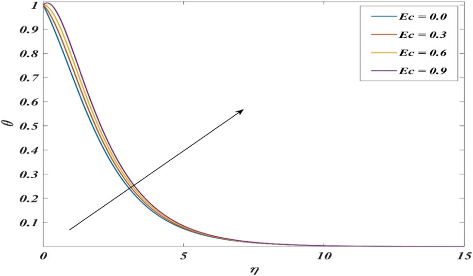
Figure 3 shows the influence of M ( M = 0.0 , 0.5 , 1.0 , 1.5 ) on motion of the velocity profile. A magnetic field exerts a force, known as the Lorentz force, on a moving charged particle. This force acts perpendicular to both the particle’s velocity and the direction of the magnetic field itself. This Lorentz force resists the fluid motion. Figure 4 depicts the impact of the Weissenberg number ( We = 0.0 , 0.1 , 0.3 , 0.5 ) on the field of flow speed. An increase in the Weissenberg number leads to a decrease in the velocity of the fluid. This is because the elastic nature of the fluid or the delayed response to shear forces creates resistance to flow.

Figures 5–13 show the temperature profiles for different values of Weissenberg number, Eckert number, and Prandtl number, thermophoresis and Brownian motion parameter, Schmidt number, reaction rate parameter, radiation parameter, and non-uniform heat source (sink) parameters, respectively. For simulation purposes, the standard fixed values for these parameters are ( Pr = 0.7 , M = 0.5 , Sc = 1.0 , γ = 0.5 , A = B = 0.1 , Nt = Nb = 0.1 , and Rd = 0.5 ) . The magnetic field strength application on the electrically conducting fluid makes it more viscous which heats up the fluid. Thus, the temperature profile rises with increasing magnetic numbers (Figure 5). The Lorentz force can also hinder the bulk flow of the nanofluid, particularly at higher magnetic field strengths. This opposition to flow can impede the movement of hot and cold regions within the fluid, potentially reducing the overall heat transfer rate.

Figure 6 describes the temperature profiles for different values for the Weissenberg number. Improving Weissenberg number leads to a rise in the temperature of nanofluids due to the formation of a thicker thermal boundary layer. A thicker boundary layer means the hot fluid layer close to the wall is confined to a smaller region. Figure 7 shows the temperature profiles for different values for radiation parameters. Increasing the radiation parameter (Rd = 0.0, 0.5, 1.0, 1.5) enhances the fluid temperature. The rate of radiative heat transfer increases dramatically with rising temperature. This relationship is governed by the Stefan–Boltzmann Law, which applies to all temperatures above absolute zero. As the temperature of the nanofluid increases, the effect of radiation becomes more dominant compared to conduction.

Figures 8 and 9 show the temperature profiles for different values of the thermophoresis and Brownian motion parameters. Increasing the Nt ( = 0.0, 0.1, 0.2, 0.3) and Nb ( = 1.0, 2.0, 3.0, 4.0) values results in enhancement of the fluid temperature. The zig–zag movement of nanoparticles produces microscopic turbulence, which leads to a temperature rise. The same phenomenon is observed in the nanofluid temperature when thermophoresis transports heat from a hotter to a colder region.

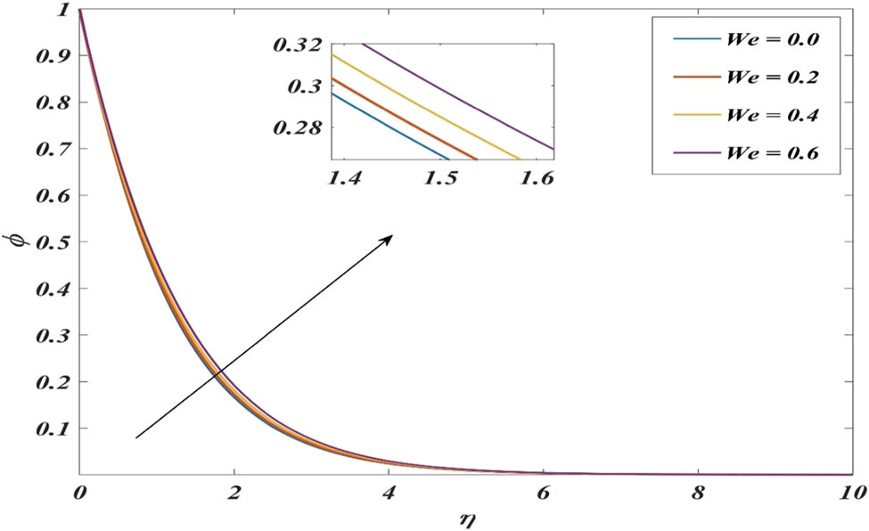
Figures 10 and 11 portray the temperature profiles for different values of a non-uniform heat source and sink parameters ( A and B ). Improving A , B = (0.0, 0.3, 0.6, 1.0) values, the temperature profiles also increase. The physical interpretation behind this is that the energy source directly heats the fluid, and hence, the local temperature of the nanofluid near the source will rise, and the presence of radiant energy is also responsible for heat enhancement. The nanofluid itself might generate heat due to internal processes such as chemical reactions. This internal heat contributes to the overall temperature rise. Figure 12 shows the temperature profiles for different values for Eckert number (Ec). As the Eckert number (Ec = 0.1, 0.5, 1.0, 1.5) improves, the internal friction of the fluid also rises, thereby enhancing the temperature of the fluid.

Figure 13 shows the Weissenberg influence on species diffusion. Augmenting We (= 0.0, 0.4, 0.8, 1.2) increases the species diffusion profiles. Figure 14 presents the parameter Nt (0.0, 0.2, 0.4, 0.6) impact on nanoparticle diffusion. It is observed that the diffusion of nanoparticles is decreased as the thermophoresis parameter escalates. As the chemical reaction parameter progresses, the species concentration of reactants decreases. The random movement of nanoparticles can counteract the concentration decrease by causing nanoparticles to move within the fluid, but their effects might be diminished by strong chemical reactions (Figure 15).

Table 3 shows the different engineering quantities affected by the flow parameters. As the Weissenberg number increases, the skin friction coefficient and the Nusselt number increase. But Sherwood's number decreases. The presence of magnetic force reduces the wall friction coefficient and heat transfer coefficient but decreases the concentration gradients. The energy source increases the energy transfer rate while the species diffusion rate decreases. The Eckert number enhances the heat and diffusion transfer rate. Increasing the chemical reaction parameter decreases the shear wall stress and energy transmission rate while the diffusion rate improves. When a species has a lower diffusivity (higher Sc), it is more susceptible to being carried by the flow (convection) rather than relying solely on its random movement (diffusion) to reach its destination. This translates to a more efficient mass transfer process, reflected by a higher Sherwood number. The random motion of nanoparticles decreases all the three engineering quantities. The wall drag coefficient and Sherwood number reduce for increasing thermophoretic parameters, whereas the Nusselt number increases.

Table 3

List of numerical values for skin friction coefficient, the local Nusselt number and local Sherwood number such as Pr = 0.7 , M = 0.5 , We = 0.1 , Sc = 1.0 , Ec = 0.1 , A = B = 0.1 , Nt = Nb = 0.1 , n p = 2,500 , η max = 20 .

We	M	A	B	Ec	γ	Sc	Nt	Nb	Cf x	Nu x	Sh x
0.0									2.14655	0.48412	1.35455
0.4									2.81216	0.48652	1.34594
0.8									2.86745	0.48720	1.34334
	0.0								1.40857	0.32242	1.36996
	0.5								1.71916	0.32356	1.36267
	1.0								1.98263	0.33565	1.35735
		0.0							1.33506	0.67823	1.41617
		0.3							1.33506	0.67956	1.47843
		0.6							1.33506	0.67965	1.54069
			0.0						1.33508	0.68965	1.47898
			0.3						1.33508	0.68985	1.46454
			0.6						1.33508	0.68960	1.45213
				0.1					1.40857	0.76852	1.40290
				0.5					1.40857	0.76952	1.47612
				1.0					1.40857	0.76982	1.58595
					0.1				1.33506	0.45685	1.38037
					0.3				1.17172	0.45582	1.44012
					0.5				1.00838	0.45466	1.55038
						1.0			1.98263	0.56324	1.35735
						1.5			1.98263	0.56325	1.48084
						2.0			1.98263	0.56325	1.58476
							0.2		1.65864	0.62531	1.46521
							0.4		1.65842	0.62542	1.46462
							0.6		1.65625	0.62452	1.45652
								0.2	1.58621	0.56112	1.35621
								0.4	1.58425	0.56021	1.35610
								0.6	1.56822	0.54125	1.34560

Figures 16–18 show the streamlines for We = ( 0.1 , 0.3 , and 0.5 ) . The starting points (We = 0.1) 1.3323 to 18.6518 and (We = 0.3) 1.2567 and 17.5963 and (We = 0.5) 1.12 and 15.6799. In each contour, it is observed that the amount of flow of energy is uniform, and the contour plot portrays a symmetry at the centre. Figures 19 and 20 show the streamlines for M ( M = 1.0 , and 2.0 ) . The starting points are (M = 1.0) 1.2241–17.1376 and (M = 2.0) 1.0974 and 15.363. The nanoparticles’ concentration is high at the centre and the flow of energy is uniform.

5 Conclusion

The purpose of this work was to examine the effects of radiation, viscous dissipation, non-uniform heat source and sink, chemical reaction, and heat and mass transfer influences on non-Newtonian nanofluid flow. To solve the formulated boundary layer equations, the Keller box method is utilized. The implications of various pertinent parameters on the flow field are numerically computed using MATLAB and portrayed as graphs and tables. These key findings can be summarized as follows:

Augmenting Weissenberg number and magnetic parameter decelerates the nanofluid velocity.
Incrementing non-uniform heat source parameters accelerates both fluid velocity and temperature. The temperature intensifies as Eckert’s number increases.
Declining species concentration profiles is noticed when thermophoresis parameter and non-uniform heat source parameters boost.
As Weissenberg’s number increases, the skin friction coefficient and Nusselt number increase, but Sherwood’s number decreases.
Enhancing energy source parameters increases the energy transfer rate, while species diffusion rate decreases. Eckert number enhances the energy and diffusion transfer rate.
Increasing chemical reaction parameters decreases the shear wall stress and energy transmission rate while the diffusion rate improves.

This problem can also be extended to add different physical impacts such as nanofluids, hybrid nanofluids, ternary hybrid nanofluids, non-Newtonian models and concentration equations, etc. In addition, we can also apply distinct schemes such as ANN, fractional derivatives, and ARA-Sumudu decomposition method [35,36,37,38,39].

Acknowledgments

The authors extend their appreciation to the Researchers Supporting Project number (RSPD2024R999), King Saud University, Riyadh, Saudi Arabia.

Funding information: This research is funded by the Scientific Deanship of Zarqa University, Jordan.
Author contributions: All authors have accepted responsibility for the entire content of this manuscript and approved its submission.
Conflict of interest: The authors state no conflict of interest.
Data availability statement: The datasets used and/or analysed during the current study are available from the corresponding author upon reasonable request.

References

[1] Hamid A, Hashim, Khan M, Alghamdi M. MHD Blasius flow of radiative Williamson nanofluid over a vertical plate. Int J Mod Phys B. 2019;33(22):1950245.10.1142/S021797921950245XSearch in Google Scholar

[2] Amanulla CH, Wakif A, Saleem S. Numerical study of a Williamson fluid past a semi-infinite vertical plate with convective heating and radiation effects. Diffus Found. 2020;28:1–15.10.4028/www.scientific.net/DF.28.1Search in Google Scholar

[3] Jalili B, Ganji AD, Jalili P, Nourazar SS, Ganji DD. Thermal analysis of Williamson fluid flow with Lorentz force on the stretching plate. Case Stud Therm Eng. 2022;39:102374.10.1016/j.csite.2022.102374Search in Google Scholar

[4] Asjad MI, Zahid M, Inc M, Baleanu D, Almohsen B. Impact of activation energy and MHD on Williamson fluid flow in the presence of bioconvection. Alex Eng J. 2022;61(11):8715–27.10.1016/j.aej.2022.02.013Search in Google Scholar

[5] Malik MY, Bilal S, Salahuddin T, Rehman KU. Three-dimensional Williamson fluid flow over a linear stretching surface. Math Sci Lett. 2017;6(1):53–61.10.18576/msl/060109Search in Google Scholar

[6] Maaitah H, Olimat AN, Quran O, Duwairi HM. Viscous dissipation analysis of Williamson fluid over a horizontal saturated porous plate at constant wall temperature. Int J Thermofluids. 2023;19:100361.10.1016/j.ijft.2023.100361Search in Google Scholar

[7] Sreenivasulu P, Poornima T, Malleswari B, Reddy NB, Souayeh B. Viscous dissipation impact on electrical resistance heating distributed Carreau nanoliquid along stretching sheet with zero mass flux. Eur Phys J Plus. 2020;135(9):705.10.1140/epjp/s13360-020-00680-6Search in Google Scholar

[8] Ramesh K, Mebarek-Oudina F, Ismail AI, Jaiswal BR, Warke AS, Lodhi RK, et al. Computational analysis on radiative non-Newtonian Carreau nanofluid flow in a microchannel under the magnetic properties. Sci Iran. 2023;30(2):376–90.10.24200/sci.2022.58629.5822Search in Google Scholar

[9] Mebarek-Oudina F, Chabani I, Vaidya H, Ismail AI. Hybrid nanofluid magneto-convective flow and porous media contribution to entropy generation. Int J Numer Methods Heat Fluid Flow. 2024;34(2):809–36. 10.1108/HFF-06-2023-0326.Search in Google Scholar

[10] Sreenivasulu P, Poornima T, Reddy NB, Reddy MG. A numerical analysis on UCM dissipated nanofluid imbedded carbon nanotubes influenced by inclined Lorentzian force along with non-uniform heat source/sink. J Nanofluids. 2019;8(5):1076–84.10.1166/jon.2019.1665Search in Google Scholar

[11] Poornima T, Sreenivasulu P, Souayeh B. Mathematical study of heat transfer in a stagnation flow of a hybrid nanofluid over a stretching/shrinking cylinder. J Eng Phys Thermophys. 2022;95(6):1443–54.10.1007/s10891-022-02613-9Search in Google Scholar

[12] Ragavi M, Poornima T. Enhanced heat transfer analysis on Ag-Al2O3/water hybrid magneto-convective nanoflow. Discov Nano. 2024;19:31. 10.1186/s11671-024-03975-0.Search in Google Scholar PubMed

[13] Konda JR, NP MR, Konijeti R, Dasore A. Effect of non-uniform heat source/sink on MHD boundary layer flow and melting heat transfer of Williamson nanofluid in porous medium. Multidiscipline Modeling Mater Struct. 2019;15(2):452–72.10.1108/MMMS-01-2018-0011Search in Google Scholar

[14] Jyotshna M, Dhanalaxmi V. Impact of Activation energy and heat source/sink on 3D flow of williamson nanofluid with gan nanoparticles over a stretching sheet. Eur J Maths Stat. 2022;3(5):16–29.10.24018/ejmath.2022.3.5.133Search in Google Scholar

[15] Song YQ, Hamid A, Sun TC, Khan MI, Qayyum S, Kumar RN, et al. Unsteady mixed convection flow of magneto-Williamson nanofluid due to stretched cylinder with significant non-uniform heat source/sink features. Alex Eng J. 2022;61(1):195–206.10.1016/j.aej.2021.04.089Search in Google Scholar

[16] Swain K, Parida SK, Dash GC. Effects of non-uniform heat source/sink and viscous dissipation on MHD boundary layer flow of Williamson nanofluid through porous medium. Defect Diffus Forum. 2018;389:110–27. Trans Tech Publications Ltd.10.4028/www.scientific.net/DDF.389.110Search in Google Scholar

[17] Sajid T, Jamshed W, Eid MR, Algarni S, Alqahtani T, Ibrahim RW, et al. Thermal case examination of inconstant heat source (sink) on viscous radiative Sutterby nanofluid flowing via a penetrable rotative cone. Case Stud Therm Eng. 2023;48:103102.10.1016/j.csite.2023.103102Search in Google Scholar

[18] Hussain SM, Eid MR, Prakash M, Jamshed W, Khan A, Alqahtani H. Thermal characterization of heat source (sink) on hybridized (Cu–Ag/EG) nanofluid flow via solid stretchable sheet. Open Phys. 2023;21(1):20220245.10.1515/phys-2022-0245Search in Google Scholar

[19] Poornima T, Sreenivasulu P, Souayeh B. Thermal radiation influence on non-Newtonian nanofluid flow along a stretchable surface with Newton boundary condition. Int J Ambient Energy. 2023;44(1):2469–79.10.1080/01430750.2023.2256329Search in Google Scholar

[20] Poornima T, Sreenivasulu P, Bhaskar Reddy N. Chemical reaction effects on an unsteady MHD mixed convective and radiative boundary layer flow over a circular cylinder. J Appl Fluid Mech. 2016;9(6):2877–85. 10.29252/jafm.09.06.24248.Search in Google Scholar

[21] Malik MY, Salahuddin T, Hussain A, Bilal S, Awais M. Homogeneous-heterogeneous reactions in Williamson fluid model over a stretching cylinder by using Keller box method. AIP Adv. 2015;5(10):107227.10.1063/1.4934937Search in Google Scholar

[22] Mahnoor S, Masood K. Cattaneo-Christov double diffusion based heat transport analysis for nanofluid flows induced by a moving plate. Numer Heat Transfer, Part A: Appl. 2023;85(3):351–63. 10.1080/10407782.2023.2186551.Search in Google Scholar

[23] Shah FA, Hussain M, Akhtar A, Inc M, Sene N, Hussan M. Impacts of chemical reaction and suction/injection on the mixed convective williamson fluid past a penetrable porous wedge. J Mathematics. 2022;2022:Article ID 3233964. 10.1155/2022/3233964.Search in Google Scholar

[24] Alrihieli H, Areshi M, Alali E, Megahed AM. MHD dissipative Williamson nanofluid flow with chemical reaction due to a slippery elastic sheet which was contained within a porous medium. Micromachines (Basel). 2022;13(11):1879. 10.3390/mi13111879.Search in Google Scholar PubMed PubMed Central

[25] Gautam AK, Verma AK, Bhattacharyya K, Mukhopadhyay S, Chamkha AJ. Impacts of activation energy and binary chemical reaction on MHD flow of Williamson nanofluid in Darcy–Forchheimer porous medium: a case of expanding sheet of variable thickness. Waves Random Complex Media. 2021;1–22. 10.1080/17455030.2021.1979274.Search in Google Scholar

[26] Sreenivasulu P, Poornima T, Reddy NB. Influence of joule heating and non-linear radiation on MHD 3D dissipating flow of casson nanofluid past a non-linear stretching sheet. Nonlinear Eng. 2019;8(1):661–72. 10.1515/nleng-2017-0143.Search in Google Scholar

[27] Rashad AM, Nafe MA, Eisa DA. Heat variation on MHD Williamson hybrid nanofluid flow with convective boundary condition and Ohmic heating in a porous material. Sci Rep. 2023;13:6071. 10.1038/s41598-023-33043-z.Search in Google Scholar PubMed PubMed Central

[28] Hussain M, Lubna A, Ashraf M, Anwar MS, Ranjha QA, Akhtar A. Ohmically dissipated MHD mixed convective flow of Williamson fluid over a penetrable stretching convective wedge with thermal radiations. Numer Heat Transfer, Part B: Fundam. 2023;1–15. 10.1080/10407790.2023.2261623.Search in Google Scholar

[29] Hussain M, Jahan S, Ranjha QA, Ahmad J, Jamil MK, Ali A. Suction/blowing impact on magneto-hydrodynamic mixed convection flow of Williamson fluid through stretching porous wedge with viscous dissipation and internal heat generation/absorption. Results Eng. 2022;16:100709. 10.1016/j.rineng.2022.100709.Search in Google Scholar

[30] Hayat T, Shafiq A, Alsaedi A. Hydromagnetic boundary layer flow of Williamson fluid in the presence of thermal radiation and Ohmic dissipation. Alex Eng J. 2016;55(3):2229–40.10.1016/j.aej.2016.06.004Search in Google Scholar

[31] Nayak MM, Mishra SR. Fuzzy parametric behaviour for the Flow of MHD Williamson nanofluid with melting heat transfer boundary condition. Int J Appl Comput Maths. 2023;9(3):18.10.1007/s40819-023-01494-7Search in Google Scholar

[32] Cebeci T, Bradshaw P. Physical and computational aspects of convective heat transfer. New York: Springer; 1984.10.1007/978-3-662-02411-9Search in Google Scholar

[33] Khan WA, Pop I. Boundary-layer flow of a nanofluid past a stretching sheet. Int J heat mass Transf. 2010;53(11–12):2477–83.10.1016/j.ijheatmasstransfer.2010.01.032Search in Google Scholar

[34] Srinivasulu T, Goud BS. Effect of inclined magnetic field on flow, heat, and mass transfer of Williamson nanofluid over a stretching sheet. Case Stud Therm Eng. 2021;23:100819.10.1016/j.csite.2020.100819Search in Google Scholar

[35] Madhu J, Saadeh R, Karthik K, Kumar RV, Kumar RN, Gowda RP, et al. Role of catalytic reactions in a flow-induced due to outer stationary and inner stretched coaxial cylinders: An application of Probabilists’ Hermite collocation method. Case Stud Therm Eng. 2024;56:104218.10.1016/j.csite.2024.104218Search in Google Scholar

[36] Saadeh R, Ahmed SA, Qazza A, Elzaki TM. Adapting partial differential equations via the modified double ARA-Sumudu decomposition method. Partial Differ Equation Appl Maths. 2023;8:100539.10.1016/j.padiff.2023.100539Search in Google Scholar

[37] Saadeh R, Ghazal B, Burqan A. A study of double general transform for solving fractional partial differential equations. Math Methods Appl Sci. 2023;46:17158–76.10.1002/mma.9493Search in Google Scholar

[38] Chandan K, Saadeh R, Qazza A, Karthik K, Varun Kumar RS, Kumar RN, et al. Predicting the thermal distribution in a convective wavy fin using a novel training physics-informed neural network method. Sci Rep. 2024;14(1):7045.10.1038/s41598-024-57772-xSearch in Google Scholar PubMed PubMed Central

[39] Qazza A, Saadeh R, Ahmed SA. ARA-sumudu method for solving volterra partial integro-differential equations. Appl Math. 2023;17(4):727–34.10.18576/amis/170421Search in Google Scholar

Received: 2024-01-09

Revised: 2024-03-28

Accepted: 2024-04-22

Published Online: 2024-06-03

This work is licensed under the Creative Commons Attribution 4.0 International License.

Articles in the same Issue

https://doi.org/10.1515/phys-2024-0036

Keywords for this article

Williamson fluid model; heat transfer; chemical reaction; magnetohydrodynamics; thermal radiation

Creative Commons

BY 4.0