Study of fractional variable-order lymphatic filariasis infection model

Mdi Begum Jeelani; Ghaliah Alhamzi; Mian Bahadur Zada; Muhammad Hassan

doi:10.1515/phys-2023-0206

Article Open Access

Study of fractional variable-order lymphatic filariasis infection model

Mdi Begum Jeelani , Ghaliah Alhamzi , Mian Bahadur Zada and Muhammad Hassan

Published/Copyright: March 20, 2024

Published by

Become an author with De Gruyter Brill

Submit Manuscript Author Information Explore this Subject

From the journal Open Physics Volume 22 Issue 1

Abstract

Variable-order derivatives are the natural extension of ordinary as well as of fractional-order differentiations and integration, respectively. Numerous suggestions for fractional variable-order operators have been made in the literature over time. Therefore, this is the moment to shine a light on the variable-order fractional calculus, due to the fact that it accurately describes the mathematical underpinnings and emphasizing the modeling utility via using contemporary numerical techniques. This study focuses on investigating a fractional variable-order model of lymphatic filariasis infection using with Atangana–Beleanue–Caputo derivative. Our investigations have led to the development of newly refined results, focusing on both qualitative and numerical aspects of analysis. To achieve our research objectives, we employ the fixed point theorems of Banach and Krasnoselskii. These theorems serve as powerful tools, allowing us to establish results regarding the existence of solutions to the model. Additionally, for precise numerical simulations, we employ the fractional Euler’s method, a sophisticated computational technique that allows us to effectively simulate and interpret the results both numerically and graphically. These graphs illustrate distinct variable-orders, providing a comprehensive understanding of the model’s behavior under different conditions. Here, it should be kept in mind that we have select various continuous functions for variable to present our graphical illustration.

Keywords: variable-order differentiation; disease dynamical model; numerical results; existence theory

1 Introduction

As a branch of mathematics, fractional calculus expands on the concepts of integer-order integration and differentiation. The purpose of fractional derivatives is to describe phenomena that are difficult to accurately model with integer-order derivatives. These phenomena often have memory or genetic characteristics, indicating that their current state depends on their entire historical trajectory rather than just their recent history [1]. This trait is common to many academic disciplines, including economics, engineering, physics, and other subjects. Fractional derivatives are an effective tool for analysis and modeling because they offer a mathematical framework for encapsulating these intricate dynamics. Recently, researchers have performed some significant work on mathematical models of various diseases. We refer few of the work [2,3].

Many researchers have used different forms of fractional differential operators to study different mathematical problems in the literature that is currently available. However, among these operators, the Caputo [4], Caputo–Fabrizio [5], and Atangana–Beleanue–Caputo (ABC) [6] fractional differential operators have become well known through their widespread use.

Their definitions rely on the standard derivative and the convolution of different kernels. It is important to remember that each definition of fractional derivative order has pros and cons.

We examine the ABC derivative, which overcomes limitations of the traditional Caputo-fractional derivative. The ABC derivative is a more comprehensive mathematical tool for describing real-world phenomena in fractional calculus. It accounts for the entire function history, making it ideal for modeling systems with memory effects. This derivative is valuable for analyzing viscoelastic materials, thermal mediums, and other substances, enabling the representation of variations across different scales. Its nonlocal nature allows for a thorough understanding of memory in various-scale structures and media, a task classical fractional derivatives cannot accomplish. ABC-fractional derivatives are anticipated to significantly impact the investigation of material microstructures, particularly those with nonlocal interactions, contributing to scientific, engineering, and technological challenges [7].

The literature contains numerous mathematical compartmental systems devised for lymphatic filariasis (LF) [8]. Various mathematical models were developed by Ottesen et al. [9] and Weerasinghe et al. [10] with distinct assumptions, including latent stage, treatment, and individuals isolation to conceptualize the transmission’s route. The parasite prevalence is independent of species or density [11]; moreover, the filarial infections carried by mosquitoes have higher mortality rates [12]. Survival of mosquito population may increase with mass drug delivery and hence transmission for an extended period of time, according to Pichon [13]. Insect population-dependent mortality might be connected with the increase intensity of infection present in the mosquito. According to the literature review, there is still a lot to learn about the infection’s transmission, and further research is required to completely understand how it spreads. The spreading of infections can be managed by proposing an appropriate measure once we gain the understanding. Also, researchers have worked on other infectious disease modeling. For instance, Thirthar [14] worked on a numerical simulation of a plant-herbivorous ecosystem, including added food-related environmental impact. Moreover, a corona virus infectious disease of 2019 model was studied by Thirthar et al. [15], and double-infected disease model in in the study of Thirthar et al. [16], and prey–predator model in in the study of Yousef et al. [17].

The fractional epidemic model for the advancement of LF considering both chronic and acute infections was formulated by Alshehri et al. [18] as :

(1) D t h 0 ABC S h ( t ) = ρ h + Ψ n I h a − B Φ h I v S h N h − μ h S h , D t h 0 ABC E h ( t ) = B Ψ h I v S h N h − ( α h + μ h ) E h , D t h 0 ABC I h a ( t ) = α h E h − Ψ n I h a − ( k + μ h ) I h a , D t h 0 ABC I h c ( t ) = k I h a − μ h I h c , D t h 0 ABC S v ( t ) = ρ h − B Φ v ( I h a + Ψ I h c ) S v N h − μ v S v , D t h 0 ABC E v ( t ) = B Φ v ( I h a + Ψ I h c ) S v N h − ( α v + μ v ) E v , D t h 0 ABC I v ( t ) = α v E v − μ v E v ,

with initial conditions,

S h ( 0 ) = S h 0 ≥ 0 , I h a ( 0 ) = I h a 0 ≥ 0 , E h ( 0 ) = E h 0 ≥ 0 , I h c ( 0 ) = I h c 0 ≥ 0 , S v ( 0 ) = S v 0 ≥ 0 , I v ( 0 ) = I v 0 ≥ 0 , and E v ( 0 ) = E v 0 ≥ 0 ,

where D t h 0 ABC is a fractional ABC derivative of order h ∈ ( 0 , 1 ] (Table 1).

Table 1

Description of the parameters used in model 1

Symbols	Interpretations
μ h	Natural death rate of humans
μ v	Natural death rate of viruses
Λ h	Recruitment rate of humans
Λ v	Recruitment rate of viruses
β	Rate of humans bitten by mosquitoes
Ψ	Real number in the unit interval (0,1)
Φ v	Transmission rate from hosts to S v
Φ h	Rate of success
φ	Rate of treated infected individuals
φ n	Susceptible rate of treated individuals

Researchers here studied numerical solutions using fixed fractional-order derivatives. As we know that variable-order derivatives produce natural extension to ordinary as well as of fractional derivatives. For situations when the orders of integration and differentiation actions are continuous functions instead of constant real or even complex number, this calculus is an extension of traditional integer-order differential calculus. Therefore, it works well for simulating the dynamics or behavior of a wide range of materials and systems, particularly diffusion-based processes. One of the interesting properties of ABC derivative is that it captures the crossover behavior in the dynamics and also generalizes the Caputo–Fabrizio derivative. The variable-order version of ABC derivatives has also used very well in various problems of fluid mechanics and chaotic models, we refer few [19,20]. For further analysis on variable-order derivatives, we refer to the study by Saxena [21].

Motivated from the variable-order ABC-fractional derivative and the LF model, we modify the LF model (1) to fractional variable-order ABC derivative as:

(2) D t ϖ ( x ) 0 ABC S h ( t ) = ρ h + Ψ n I h a − B Φ h I v S h N h − μ h S h , D t ϖ ( x ) 0 ABC E h ( t ) = B Ψ h I v S h N h − ( α h + μ h ) E h , D t ϖ ( x ) 0 ABC I h a ( t ) = α h E h − Ψ n I h a − ( k + μ h ) I h a , D t ϖ ( x ) 0 ABC I h c ( t ) = k I h a − μ h I h c , D t ϖ ( x ) 0 ABC S v ( t ) = ρ h − B Φ v ( I h a + Ψ I h c ) S v N h − μ v S v , D t ϖ ( x ) 0 ABC E v ( t ) = B Φ v ( I h a + Ψ I h c ) S v N h − ( α v + μ v ) E v , D t ϖ ( x ) 0 ABC I v ( t ) = α v E v − μ v E v ,

with the same initial conditions as mentioned earlier in model (1), where ϖ : [ 0 , △ ] → ( 0 , 1 ] is the continuous function and D t ϖ ( x ) 0 ABC is the ABC-fractional variable-order derivative. Existence theory of variable-order problems and stability analysis are the main crucial aspects of differential equations that have been studied very well. For the existence theory, usually we use fixed point theory [22,23]. In case of stability analysis nonlinear functional analysis helps very well. Hyers–Ulam stability concepts in this regard a useful concept to be investigated for the stability of solution for problems under consideration. Here, we apply the procedures given in Krasnoselskii [24] and Shah et al. [25]. Furthermore, to simulate our results, we extend the Euler method given by Zine et al. [26]. Various graphical illustrations are given using various continuous functions for variable-order.

Our manuscript is organized as: Section 1 is devoted to literature and introduction. Section 2 contains basic results. Section 3 contains the results devoted to qualitative theory and stability analysis. Section 4 contains numerical procedure and its utilization to simulate the results graphically. Section 5 is devoted to conclusion.

2 Preliminaries

Some basic results are recollected as:

Definition 2.1

[19] If f : R + → R and α ∈ ( n − 1 , n ] , ∀ n ∈ N , then

(3) D t α C ( f ( t ) ) = 1 Γ ( m − α ) ∫ a t ( t − τ ) m − α − 1 f n ( τ ) d τ ,

where Γ is the gamma function, is called the Caputo fractional derivative of order α , provided it exists.

Definition 2.2

[20] The ABC-fractional derivative is defined by:

(4) 0 A B C D a + α D a + α 0 ABC ( g ( t ) ) = N ( α ) 1 − α ∫ a t g ′ ( y ) E α α α − 1 ( t − y ) α d y ,

where α ∈ [ 0 , 1 ] , a < t < b , g is a differentiable function on [ a , b ] such that g ′ ∈ L 1 ( a , b ) , N ( α ) is a normalization function satisfying N ( 0 ) = N ( 1 ) = 1 and E α the generalized Mittag–Leffler function E α = E α ( − t α ) = ∑ k = 0 ∞ ( − t ) α k Γ ( α k + 1 ) .

Definition 2.3

[19] The ABC fractional derivative with variable-order ϖ ( x ) in Liouville–Caputo sense is defined as:

(5) D t ϖ ( x ) 0 ABC ( f ( t ) ) = N ( ϖ ( x ) ) 1 − ϖ ( x ) ∫ 0 t E ϖ ( x ) − ϖ ( x ) ( t − τ ) ϖ ( x ) 1 − ϖ ( x ) f ′ ( τ ) d τ ,

where n − 1 < ϖ ( x ) ≤ n and N ( ϖ ( x ) ) = 1 − ϖ ( x ) + ϖ ( x ) Γ ( ϖ ( x ) ) is a normalization function. Related integral can be formulated as:

(6) I t ϖ ( x ) 0 ABC ( f ( t ) ) = 1 − ϖ ( x ) N ( ϖ ( x ) ) f ( t ) + ϖ ( x ) N ( ϖ ( x ) ) Γ ( ϖ ( x ) ) ∫ 0 t ( t − y ) ϖ ( x ) − 1 f ( y ) d y ,

where n − 1 < ϖ ( x ) ≤ n .

Lemma 2.3.1

[19] The integral representation of

(7) D t ϖ ( x ) ABC ψ ( t ) = ξ ( t ) , ψ ( 0 ) = ψ 0

(8) ψ ( t ) = ψ 0 + 1 − ϖ ( x ) N ( ϖ ( x ) ) ξ ( t ) + ϖ ( x ) N ( ϖ ( x ) ) Γ ( ϖ ( x ) ) ∫ 0 t ( t − y ) ϖ ( x ) − 1 ξ ( y ) d y .

The fractional variable-order ABC derivative and the associated AB integral are related by:

( I a ϖ ( x ) AB ) ( D a ϖ ( x ) ABC ) f ( t ) = f ( t ) − f ( a ) .

Theorem 2.4

[24] Let N be nonempty, convex, and closed a subset of a Banach space B . If the mappings F 1 , F 2 : N → B satisfy the following conditions:

F 1 u + F 2 v ∈ N , ∀ u , v ∈ N ;
F 1 is contraction mapping;
F 2 is compact and continuous.

Then, there exists x * ∈ N such that F 2 x * + F 1 x * = x * .

Definition 2.5

[25] Let T be an operator on a Banach space X . Then, the fixed point equation

(9) x = T x ,

is said to be Ulam–Hyers stable if there exists a real number c T > 0 such that for each ε > 0 and each solution y ∗ of the inequality:

(10) ‖ T y − y ‖ < ε ,

there exists a solution x ∗ of Eq. (9) such that

(11) ‖ x ∗ − y ∗ ‖ ≤ c T ⋅ ε .

3 Qualitative analysis

We split this section into two subsections as follows:

3.1 Existence theory

In this section, we study the existence and uniqueness of the fractional variable-order LF model (2). To perform fractional analysis on the LF model, we define f = ( S h , E h , I h a , I h c , S v , E v , I v ) and B = [ 0 , △ ] , where 0 ≤ t ≤ △ ≤ ∞ . Then, Ξ = C ( B , R 7 ) is a Banach space with supremum norm:

(12) ‖ f ‖ = sup t ∈ B { ∣ f ( t ) ∣ : f ∈ Ξ } ,

where ∣ f ∣ = ∣ S h ∣ + ∣ E h ∣ + ∣ I h a ∣ + ∣ I h c ∣ + ∣ S v ∣ + ∣ E v ∣ + ∣ I v ∣ . Also, S h , E h , I h a , I h c , S v , E v , I v , N ∈ C [ 0 , △ ] . With the help of fixed point theory, we check the existence and uniqueness of LF model (2). For this purpose, we reformulate the LF model (2) as:

D t ϖ ( x ) ABC S h ( t ) = Ξ 1 ( S h , E h , I h c , I h a , S v , I v , E v ) , D t ϖ ( x ) ABC E h ( t ) = Ξ 2 ( S h , E h , I h c , I h a , S v , I v , E v ) , D t ϖ ( x ) ABC I h a ( t ) = Ξ 3 ( S h , E h , I h c , I h a , S v , I v , E v ) , D t ϖ ( x ) ABC I h c ( t ) = Ξ 4 ( S h , E h , I h c , I h a , S v , I v , E v ) , D t ϖ ( x ) ABC S v ( t ) = Ξ 5 ( S h , E h , I h c , I h a , S v , I v , E v ) , D t ϖ ( x ) ABC E v ( t ) = Ξ 6 ( S h , E h , I h c , I h a , S v , I v , E v ) , D t ϖ ( x ) ABC I v ( t ) = Ξ 7 ( S h , E h , I h c , I h a , S v , I v , E v ) ,

where

(13) Ξ 1 ( S h , E h , I h c , I h a , S v , I v , E v ) = ρ h + Ψ n I h a − B Φ h I v S h N h − μ h S h , Ξ 2 ( S h , E h , I h c , I h a , S v , I v , E v ) = B Ψ h I v S h N h − ( α h + μ h ) E h , Ξ 3 ( S h , E h , I h c , I h a , S v , I v , E v ) = α h E h − Ψ n I h a − ( k + μ h ) I h a , Ξ 4 ( S h , E h , I h c , I h a , S v , I v , E v ) = k I h a − μ h I h c , Ξ 5 ( S h , E h , I h c , I h a , S v , I v , E v ) = ρ h − B Φ v ( I h a + Ψ I h c ) S v N h − μ v S v , Ξ 6 ( S h , E h , I h c , I h a , S v , I v , E v ) = B Φ v ( I h a + Ψ I h c ) S v N h − ( α v + μ v ) E v , Ξ 7 ( S h , E h , I h c , I h a , S v , I v , E v ) = α v E v − μ v E v .

Let us consider System (2) as:

(14) D t ϖ ( x ) ABC f ( t ) = Ξ ( t , f ( t ) ) ,

with initial condition f ( 0 ) = f 0 ≥ 0 . Note that

(15) f ( t ) = ( S h , E h , I h c , I h a , S v , I v , E v ) T , f 0 = ( S h 0 , E h 0 , I h a 0 , I h c 0 , S v 0 , E v 0 , I v 0 ) T , Ξ ( t , f ( t ) ) = ( Ξ n ( t , S h , E h , I h c , I h a , S v , I v , E v ) ) T , n = 1 , 2 , 3 , 4 , 5 , 6 , 7 .

In Eq. (15), the transpose is represented by the superscript T . By using Lemma 2.3.1, Eq. (14) becomes

(16) f ( t ) = f 0 + 1 − ϖ ( x ) N ( ϖ ( x ) ) Ξ ( t , f ( t ) ) + ϖ ( x ) N ( ϖ ( x ) ) Γ ( ϖ ( x ) ) ∫ 0 t ( t − y ) ϖ ( x ) − 1 Ξ ( y , f ( y ) ) d y .

To proceed further, based on Lipschitzian and some growth condition assumptions, we consider the two hypotheses:

For two constants P and Q , we have
∣ Ξ ( t , f ( t ) ) ∣ ≤ P ‖ f ‖ + Q , ∀ t ∈ [ 0 , △ ] .
For a constant M E > 0 and for each f 1 , f 2 ∈ B , we have
∣ Ξ ( t , f 1 ) − Ξ ( t , f 2 ) ∣ ≤ M E ∥ f 1 − f 2 ∥ , ∀ t ∈ [ 0 , △ ] .

For ε = β 2 1 − β 1 with β 1 = 1 − ϖ ( x ) N ( ϖ ( x ) ) + t ϖ ( x ) N ( ϖ ( x ) ) Γ ( ϖ ( x ) ) P < 1 , β 2 = ∣ f 0 ∣ + 1 − ϖ ( x ) N ( ϖ ( x ) ) + t ϖ ( x ) N ( ϖ ( x ) ) Γ ( ϖ ( x ) ) Q and for each f ∈ B , t ∈ [ 0 , △ ] , we let F ε = { f ∈ B : ‖ f ‖ ≤ ε } . Let F = F 1 + F 2 , where the two operators F 1 and F 2 are defined by:

(17) F 1 f ( t ) = f 0 + 1 − ϖ ( x ) N ( ϖ ( x ) ) Ξ ( t , f ( t ) )

and

(18) F 2 f ( t ) = ϖ ( x ) N ( ϖ ( x ) ) Γ ( ϖ ( x ) ) ∫ 0 t ( t − y ) ϖ ( x ) − 1 Ξ ( y , f ( y ) ) d y .

Theorem 3.1

Prove that F 1 f 1 + F 2 f 2 ∈ F ε , for all f 1 , f 2 ∈ F ε .

Proof

For every f 1 , f 2 ∈ F ε , we have

∣ F 1 f 1 ( t ) + F 2 f 2 ( t ) ∣ = f 0 + 1 − ϖ ( x ) N ( ϖ ( x ) ) Ξ ( t , f 1 ( t ) ) + ϖ ( x ) N ( ϖ ( x ) ) Γ ( ϖ ( x ) ) ∫ 0 t ( t − y ) ϖ ( x ) − 1 Ξ ( y , f 2 ( y ) ) d y ≤ ∣ f 0 ∣ + 1 − ϖ ( x ) N ( ϖ ( x ) ) ∣ Ξ ( t , f 1 ( t ) ) ∣ + ϖ ( x ) N ( ϖ ( x ) ) Γ ( ϖ ( x ) ) ∫ 0 t ( t − y ) ϖ ( x ) − 1 ∣ Ξ ( y , f 2 ( y ) ) ∣ d y ≤ ∣ f 0 ∣ + 1 − ϖ ( x ) N ( ϖ ( x ) ) [ P ‖ f 1 ‖ + Q ] + ϖ ( x ) N ( ϖ ( x ) ) Γ ( ϖ ( x ) ) ∫ 0 t ( t − y ) ϖ ( x ) − 1 [ P ‖ f 2 ‖ + Q ] d y = ∣ f 0 ∣ + 1 − ϖ ( x ) N ( ϖ ( x ) ) [ P ‖ f 1 ‖ + Q ] + [ P ‖ f 2 ‖ + Q ] ϖ ( x ) N ( ϖ ( x ) ) Γ ( ϖ ( x ) ) ∫ 0 t ( t − y ) ϖ ( x ) − 1 d y ≤ ∣ f 0 ∣ + 1 − ϖ ( x ) N ( ϖ ( x ) ) [ P ε + Q ] + [ P ε + Q ] t ϖ ( x ) N ( ϖ ( x ) ) Γ ( ϖ ( x ) ) = ∣ f 0 ∣ + 1 − ϖ ( x ) N ( ϖ ( x ) ) + t ϖ ( x ) N ( ϖ ( x ) ) Γ ( ϖ ( x ) ) [ P ε + Q ] = ∣ f 0 ∣ + 1 − ϖ ( x ) N ( ϖ ( x ) ) + t ϖ ( x ) N ( ϖ ( x ) ) Γ ( ϖ ( x ) ) Q + 1 − ϖ ( x ) N ( ϖ ( x ) ) + t ϖ ( x ) N ( ϖ ( x ) ) Γ ( ϖ ( x ) ) P ε .

Taking supremum of both sides, we obtain

∥ F 1 f 1 + F 2 f 2 ∥ ≤ ∣ f 0 ∣ + 1 − ϖ ( x ) N ( ϖ ( x ) ) + t ϖ ( x ) N ( ϖ ( x ) ) Γ ( ϖ ( x ) ) Q + 1 − ϖ ( x ) N ( ϖ ( x ) ) + t ϖ ( x ) N ( ϖ ( x ) ) Γ ( ϖ ( x ) ) P ε = β 1 + β 2 ε ≤ ε .

This confirms that F 1 f 1 + F 2 f 2 ∈ F ε .□

Theorem 3.2

Prove that F 1 is a contraction.

Proof

To prove that F 1 is a contraction. Let f , f * ∈ F ε * , then by using hypothesis ( H 2 ) , we have

∣ F 1 f ( t ) − F 1 f * ( t ) ∣ = 1 − ϖ ( x ) N ( ϖ ( x ) ) [ Ξ ( t , f ( t ) ) − Ξ ( t , f * ( t ) ) ] ≤ 1 − ϖ ( x ) N ( ϖ ( x ) ) ∣ Ξ ( t , f ( t ) ) − Ξ ( t , f * ( t ) ) ∣ ≤ 1 − ϖ ( x ) N ( ϖ ( x ) ) M E ∥ f − f * ∥ .

Taking supremum of both sides, we obtain

∥ F 1 f − F 1 f * ∥ ≤ 1 − ϖ ( x ) N ( ϖ ( x ) ) M E ∥ f − f * ∥ .

But 1 − ϖ ( x ) N ( ϖ ( x ) ) M E < 1 . Hence, F 1 is contraction.□

Theorem 3.3

Prove that F 2 is continuous and compact.

Proof

To show that F 2 is continuous. Let f n be a sequence in F ε converging to a point f ∈ F ε . Then, for all t ∈ [ 0 , △ ] , we have

lim n → ∞ F 2 { f n } ( t ) = ϖ ( x ) N ( ϖ ( x ) ) Γ ( ϖ ( x ) ) lim n → ∞ × ∫ 0 t ( t − y ) ϖ ( x ) − 1 Ξ ( y , f n ( y ) ) d y .

By the Lebesuge-dominated convergence theorem, we can write

lim n → ∞ F 2 { f n } ( t ) = ϖ ( x ) N ( ϖ ( x ) ) Γ ( ϖ ( x ) ) × ∫ 0 t ( t − y ) ϖ ( x ) − 1 lim n → ∞ Ξ ( y , f n ( y ) ) d y = ϖ ( x ) N ( ϖ ( x ) ) Γ ( ϖ ( x ) ) ∫ 0 t ( t − y ) ϖ ( x ) − 1 Ξ ( y , f ( y ) ) d y = F 2 f ( t ) .

Thus, F 2 is continuous. Next, we check the uniformly boundedness of F 2 . For this, we have

∣ F 2 f ( t ) ∣ = ϖ ( x ) N ( ϖ ( x ) ) Γ ( ϖ ( x ) ) ∫ 0 t ( t − y ) ϖ ( x ) − 1 [ Ξ ( y , f ( y ) ) ] d y ≤ ϖ ( x ) N ( ϖ ( x ) ) Γ ( ϖ ( x ) ) ∫ 0 t ( t − y ) ϖ ( x ) − 1 ∣ Ξ ( y , f ( y ) ) ∣ d y ≤ ϖ ( x ) N ( ϖ ( x ) ) Γ ( ϖ ( x ) ) ∫ 0 t ( t − y ) ϖ ( x ) − 1 [ P ‖ f ‖ + Q ] d y = ϖ ( x ) [ P ‖ f ‖ + Q ] N ( ϖ ( x ) ) Γ ( ϖ ( x ) ) ∫ 0 t ( t − y ) ϖ ( x ) − 1 d y = t ϖ ( x ) N ( ϖ ( x ) ) Γ ( ϖ ( x ) ) ( P ‖ f ‖ + Q ) .

Taking supremum of both sides, we obtain

∥ F 2 f ∥ ≤ t ϖ ( x ) N ( ϖ ( x ) ) Γ ( ϖ ( x ) ) [ P ε + Q ] .

Thus, F 2 is uniformly bounded on F ε . Next, to show that F 2 is equicontinuous. For this, let t 1 , t 2 ∈ [ 0 , △ ] with t 1 < t 2 . Then, we have

∣ F 2 f ( t 2 ) − F 2 f ( t 1 ) ∣ = ϖ ( x ) N ( ϖ ( x ) ) Γ ( ϖ ( x ) ) ∫ 0 t 2 ( t 2 − y ) ϖ ( x ) − 1 Ξ ( y , f ( y ) ) d y − ϖ ( x ) N ( ϖ ( x ) ) Γ ( ϖ ( x ) ) ∫ 0 t 1 ( t 1 − y ) ϖ ( x ) − 1 Ξ ( y , f ( y ) ) d y ≤ ϖ ( x ) N ( ϖ ( x ) ) Γ ( ϖ ( x ) ) ∫ t 1 t 2 ( t 2 − y ) ϖ ( x ) − 1 ∣ Ξ ( y , f ( y ) ) ∣ d y + ϖ ( x ) N ( ϖ ( x ) ) Γ ( ϖ ( x ) ) ∫ 0 t 1 [ ( t 2 − y ) ϖ ( x ) − 1 − ( t 1 − y ) ϖ ( x ) − 1 ] ∣ Ξ ( y , f ( y ) ) ∣ d y ≤ ϖ ( x ) N ( ϖ ( x ) ) Γ ( ϖ ( x ) ) ∫ t 1 t 2 ( t 2 − y ) ϖ ( x ) − 1 [ P ‖ f ‖ + Q ] d y + ϖ ( x ) N ( ϖ ( x ) ) Γ ( ϖ ( x ) ) ∫ 0 t 1 [ ( t 2 − y ) ϖ ( x ) − 1 − ( t 1 − y ) ϖ ( x ) − 1 ] [ P ‖ f ‖ + Q ] d y = [ P ‖ f ‖ + Q ] ϖ ( x ) N ( ϖ ( x ) ) Γ ( ϖ ( x ) ) ∫ t 1 t 2 ( t 2 − y ) ϖ ( x ) − 1 d y + [ P ‖ f ‖ + Q ] ϖ ( x ) N ( ϖ ( x ) ) Γ ( ϖ ( x ) ) ∫ 0 t 1 [ ( t 2 − y ) ϖ ( x ) − 1 − ( t 1 − y ) ϖ ( x ) − 1 ] d y = [ P ‖ f ‖ + Q ] ϖ ( x ) N ( ϖ ( x ) ) Γ ( ϖ ( x ) ) ∫ t 1 t 2 ( t 2 − y ) ϖ ( x ) − 1 d y + [ P ‖ f ‖ + Q ] ϖ ( x ) N ( ϖ ( x ) ) Γ ( ϖ ( x ) ) ∫ 0 t 2 ( t 2 − y ) ϖ ( x ) − 1 d y − [ P ‖ f ‖ + Q ] ϖ ( x ) N ( ϖ ( x ) ) Γ ( ϖ ( x ) ) ∫ 0 t 1 ( t 1 − y ) ϖ ( x ) − 1 d y ≤ [ P ε + Q ] N ( ϖ ( x ) ) Γ ( ϖ ( x ) ) ( ( t 2 − t 1 ) ϖ ( x ) + ( t 1 ϖ ( x ) − t 2 ϖ ( x ) ) + ( t 2 − t 1 ) ϖ ( x ) ) = [ P ε + Q ] N ( ϖ ( x ) ) Γ ( ϖ ( x ) ) ( 2 ( t 2 − t 1 ) ϖ ( x ) + ( t 2 ϖ ( x ) − t 1 ϖ ( x ) ) ) .

Taking limit as t 1 ⟶ t 2 , we obtain

∣ F 2 f ( t 2 ) − F 2 f ( t 1 ) ∣ ⟶ 0 ,

i.e., F 2 is equi-continuous. Using the Arzelá–Ascoli theorem, F 2 is relatively compact and thus completely continuous. Consequently, F 2 is compact□

Theorem 3.4

Eq. (14) has a solution under the assumptions ( H 1 ) and ( H 2 ) .

Proof

Note that f ( t ) satisfies Eq. (16) if and only if f ( t ) is a solution of Eq. (14). Therefore, to determine the solution for Eq. (14), it suffices to identify the solution for Eq. (16). For this purpose, we convert Eq. (16) to the operator equation:

(19) f ( t ) = F 1 f ( t ) + F 2 f ( t ) .

Hence, it is essential to demonstrate that the operator equation fulfills all the requirements outlined in Theorem 2.4. To check this, we have, clearly, that F ε is nonempty, convex, closed, and bounded. With the help of Theorems 3.1–3.3, the conditions of Theorem 2.4 holds. Thus, there exist f * ∈ F ε such that

f * = F 1 f * + F 2 f * ,

i.e., f * is the solution of Eq. (19); consequently, f * is the solution of Eq. (14).□

Theorem 3.5

Prove the uniqueness of the solution for integral Eq. (14) provided β 3 = 1 − ϖ ( x ) N ( ϖ ( x ) ) + t ϖ ( x ) N ( ϖ ( x ) ) Γ ( ϖ ( x ) ) M E < 1 , considering the assumption ( H 2 ) .

Proof

Since F : B ⟶ B is defined by:

(20) f ( t ) = F 1 f ( t ) + F 2 f ( t ) = F f ( t ) = f 0 + 1 − ϖ ( x ) N ( ϖ ( x ) ) Ξ ( t , f ( t ) ) + ϖ ( x ) N ( ϖ ( x ) ) Γ ( ϖ ( x ) ) ∫ 0 t ( t − y ) ϖ ( x ) − 1 Ξ ( y , f ( y ) ) d y .

Now, for t ∈ [ 0 , △ ] and f , f * ∈ B , it follows that

∣ F f ( t ) − F f * ( t ) ∣ = 1 − ϖ ( x ) N ( ϖ ( x ) ) ( Ξ ( t , f ( t ) ) − Ξ ( t , f * ( t ) ) ) + ϖ ( x ) N ( ϖ ( x ) ) Γ ( ϖ ( x ) ) ∫ 0 t ( t − y ) ϖ ( x ) − 1 × ( Ξ ( y , f ( y ) ) − Ξ ( y , f * ( y ) ) ) d y ∣ ≤ 1 − ϖ ( x ) N ( ϖ ( x ) ) ∣ Ξ ( t , f ( t ) ) − Ξ ( t , f * ( t ) ) ∣ + M E ∥ f − f * ∥ ϖ ( x ) N ( ϖ ( x ) ) Γ ( ϖ ( x ) ) ∫ 0 t ( t − y ) ϖ ( x ) − 1 d y ≤ 1 − ϖ ( x ) N ( ϖ ( x ) ) ∣ Ξ ( t , f ( t ) ) − Ξ ( t , f * ( t ) ) ∣ + M E ∥ f − f * ∥ ϖ ( x ) N ( ϖ ( x ) ) Γ ( ϖ ( x ) ) ∫ 0 t ( t − y ) ϖ ( x ) − 1 d y ≤ 1 − ϖ ( x ) N ( ϖ ( x ) ) + t ϖ ( x ) N ( ϖ ( x ) ) Γ ( ϖ ( x ) ) M E ∥ f − f * ∥ .

Taking supremum of both sides, we obtain

∥ F f − F f * ∥ ≤ 1 − ϖ ( x ) N ( ϖ ( x ) ) + t ϖ ( x ) N ( ϖ ( x ) ) Γ ( ϖ ( x ) ) M E ∥ f − f * ∥ .

Therefore, the implication of β 3 suggests that F is contraction. Consequently, Eq. (16) possesses a unique solution, leading to the conclusion that System (14) also has a unique solution.□

3.2 Ulam–Hyers stability for LF model

The assessment of stability in nonlinear dynamical models is essential. Therefore, within this section, we utilize the Ulam–Hyers stability principle to analyze the LF model denoted by (14) with some nonlinear functional analysis concepts. Occasionally, the analysis of stability is related to various types of equations, including ordinary or partial differential equations, integral equations, and functional equations.

Definition 3.6

The LF model (14) is Ulam–Hyers stable if one can find λ > 0 such that for ε > 0 and for each solution f ˜ ∈ B of the inequality:

(21) ∣ D t ϖ ( x ) ABC f ˜ ( t ) − Ξ ( T , f ˜ ( t ) ) ∣ ≤ λ , ∀ t ∈ [ 0 , △ ] .

There exists a solution f ∈ B to problem (14) with an initial condition f ( 0 ) = f ˜ ( 0 ) and the property

(22) ∣ f ˜ ( t ) − f ( t ) ∣ ≤ ε λ , ∀ t ∈ [ 0 , △ ]

where

(23) f ˜ ( t ) = ( S ˜ h , E ˜ h , I ˜ h a , I ˜ h c , S ˜ v , E ˜ v , I v ˜ ) T , f ˜ 0 = ( S ˜ h 0 , E ˜ h 0 , I ˜ h a 0 , I ˜ h c 0 , S ˜ v 0 , E ˜ v 0 , I ˜ v 0 ) T , Ξ ( t , f ˜ ( t ) ) = ( Ξ n ( t , S ˜ h , E ˜ h , I ˜ h a , I ˜ h c , S ˜ v , E ˜ v , I v ˜ ) T , n = 1 , 2 , 3 , 4 , 5 , 6 , 7 .

Remark 1

Let f ∈ C [ 0 , △ ] , which is a small perturbation with f ( 0 ) = 0 such that ∣ f ( t ) ∣ ≤ λ , for t ∈ [ 0 , △ ] and λ > 0 . Then, the model (14) becomes

(24) D t ϖ ( x ) ABC f ˜ ( t ) = Ξ ( t , f ˜ ( t ) ) + f ( t ) ,

where f ( t ) = ( f 1 ( t ) , f 2 ( t ) , f 3 ( t ) , f 4 ( t ) , f 5 ( t ) , f 6 ( t ) , f 7 ( t ) ) T .

Lemma 3.6.1

The perturbed system (24)

with initial condition f ˜ ( 0 ) = f ˜ 0

has a solution if the following inequality is satisfied

(25) ∣ f ˜ f ( t ) − f ˜ ( t ) ∣ ≤ l λ ,

where f ˜ f ( t ) is the solution of System (24) and l = Γ ( ϖ ( x ) ) ( 1 − ϖ ( x ) ) + t ϖ ( x ) N ( ϖ ( x ) Γ ( ϖ ( x ) ) ) .

Proof

Utilizing Remark 1 along with Lemma 2.3.1, the solution to System (24) can be expressed as follows:

f ˜ f ( t ) = f ˜ 0 + 1 − ϖ ( x ) N ( ϖ ( x ) ) Ξ ( t , f ˜ ( t ) ) + ϖ ( x ) N ( ϖ ( x ) ) Γ ( ϖ ( x ) ) ∫ 0 t ( t − y ) ϖ ( x ) − 1 Ξ ( y , f ˜ ( y ) ) d y + 1 − ϖ ( x ) N ( ϖ ( x ) ) f ( t ) + ϖ ( x ) N ( ϖ ( x ) ) Γ ( ϖ ( x ) ) × ∫ 0 t ( t − y ) ϖ ( x ) − 1 Ξ ( y ) d y .

Also, we know that

f ˜ ( t ) = f ˜ 0 + 1 − ϖ ( x ) N ( ϖ ( x ) ) Ξ ( t , f ˜ ( t ) ) + ϖ ( x ) N ( ϖ ( x ) ) Γ ( ϖ ( x ) ) ∫ 0 t ( t − y ) ϖ ( x ) − 1 Ξ ( y , f ˜ ( y ) ) d y .

The observation in Remark 1 implies that

(26)□ ∣ f ˜ f ( t ) − f ˜ ( t ) ∣ ≤ 1 − ϖ ( x ) N ( ϖ ( x ) ) ∣ f ( t ) ∣ + ϖ ( x ) N ( ϖ ( x ) ) Γ ( ϖ ( x ) ) × ∫ 0 t ( t − y ) ϖ ( x ) − 1 ∣ f ( y ) ∣ d y ≤ Γ ( ϖ ( x ) ) ( 1 − ϖ ( x ) ) + t ϖ ( x ) N ( ϖ ( x ) ) Γ ( ϖ ( x ) ) λ = l λ .

Theorem 3.7

The LF system (14) is Ulam–Hyers stable in B under the assumption ( H 2 ) .

Proof

In Section 3, we have proved that the LF system (14) has a unique solution:

(27) f ( t ) = f 0 + 1 − ϖ ( x ) N ( ϖ ( x ) ) Ξ ( t , f ( t ) ) + ϖ ( x ) N ( ϖ ( x ) ) Γ ( ϖ ( x ) ) ∫ 0 t ( t − y ) ϖ ( x ) − 1 Ξ ( y , f ( y ) ) d y .

Also, f ˜ ∈ B is the solution of inequality (21). Thus by suggested initial condition f ( 0 ) = f ˜ ( 0 ) , Eq. (27) becomes

(28) f ˜ ( t ) = f ˜ 0 + 1 − ϖ ( x ) N ( ϖ ( x ) ) Ξ ( t , f ˜ ( t ) ) + ϖ ( x ) N ( ϖ ( x ) ) Γ ( ϖ ( x ) ) ∫ 0 t ( t − y ) ϖ ( x ) − 1 Ξ ( y , f ˜ ( y ) ) d y .

Now, employing Lemma 3.6.1 and assumption ( H 2 ) , we obtain

(29) ∣ f ˜ ( t ) − f ( t ) ∣ ≤ ∣ f ˜ ( t ) − f ˜ f ( t ) ∣ + ∣ f ˜ f ( t ) − f ( t ) ∣ ≤ l λ + 1 − ϖ ( x ) N ( ϖ ( x ) ) ∣ Ξ ( t , f ˜ ( t ) ) − Ξ ( t , f ( t ) ) ∣ + ϖ ( x ) N ( ϖ ( x ) ) Γ ( ϖ ( x ) ) ∫ 0 t ( t − y ) ϖ ( x ) − 1 × ∣ Ξ ( t , f ˜ ( t ) ) − Ξ ( t , f ( t ) ) ∣ d y + l λ ≤ 2 l λ + 1 − ϖ ( x ) N ( ϖ ( x ) ) + t ϖ ( x ) N ( ϖ ( x ) ) Γ ( ϖ ( x ) ) × M E ‖ f ˜ − f ‖ ,

which implies that

(30) ‖ f ˜ − f ‖ ≤ 2 l λ 1 − β 3 ⋅

If we choose ε = 2 l 1 − β 3 , we obtain

(31) ‖ f ˜ − f ‖ ≤ λ ⋅ ε .

Hence, the LF system (14) is Ulam–Hyers stable.□

4 Numerical solution

We will address the numerical solution of the fractional LF model in this section. Numerous numerical approaches exist for computing the numerical outcomes of a fractional differential equation system. However, even Euler’s method is applicable for analyzing its solution in this scenario. To achieve this, we will implement Euler’s method for the resolution of the fractional LF model (14).

Zine et al. [26] demonstrated the generalized Taylor’s formula for the ABC-fractional derivative, which is given by:

(32) f ( x ) = ∑ m = o n ( D m δ a ABC f ( a ) ) ∑ j = 0 m × m j τ ( δ ) m − j f ( δ ) j ( x − a ) j δ Γ ( j δ + 1 ) + ( D ( n + 1 ) δ a ABC f ( ε ) ) ∑ j = 0 n + 1 × n + 1 j τ ( δ ) n + 1 − j f ( δ ) j ( x − a ) j δ Γ ( j δ + 1 ) .

Consider the initial value problem, we have

(33) D t ϖ ( x ) ABC f ( t ) = Ξ ( t , f ( t ) ) , f ( 0 ) = f 0 ,

where ϖ : [ 0 , △ ] → ( 0 , 1 ] . Consider the interval [ 0 , a ) over which we seek to derive a solution for our given problem. To facilitate generalization, we opt for ( t m , f ( t m ) ) instead of [ 0 , a ) and employ it for our approximation process. Suppose that the interval is divided into j subintervals of uniform width, where h = a ∕ j , and utilize nodes t m = m h for m = 0 , 1 , … , j . Assuming that f ( t ) , D t a ABC f ( t ) , etc. exhibit continuity on ( t m , f ( t m ) ) , we can apply Eq. (33) to expand f ( t ) about t = t 0 as follows:

(34) f ( t 1 ) = f ( t 0 ) + D t ϖ ( x ) ABC f ( t 0 ) ϖ ( x ) ( t 1 − a ) ϖ ( x ) Γ ( ϖ ( x ) + 1 ) N ( ϖ ( x ) ) + ⋯ .

Through the omission of higher-order terms due to the considered step size h being the smallest positive number and assuming h = t 1 , D t ϖ ( x ) ABC f ( t 0 ) = Ξ ( t 0 , f ( t 0 ) ) , Eq. (34) becomes

(35) f ( t 1 ) = f ( t 0 ) + Ξ ( t 0 , f ( t 0 ) ) × ϖ ( x ) ( h − a ) ϖ ( x ) Γ ( ϖ ( x ) + 1 ) N ( ϖ ( x ) ) .

Eq. (35) transforms into the iterative formula used to iteratively compute the values of t that provide an approximation for the solution of f ( t ) . As a result, the overall structure of the fractional Euler’s approach for solving initial value problems involving the ABC fractional derivative can be summarized as follows:

(36) t m + 1 = t m + h ,

(37) f ( t m + 1 ) = f ( t m ) + Ξ ( t m , f ( t m ) ) ϖ ( x ) ( h − a ) ϖ ( x ) Γ ( ϖ ( x ) + 1 ) N ( ϖ ( x ) ) ⋅

One can readily note that when ϖ ( x ) = 1 , the aforementioned equation corresponds to the classical Euler’s method. The compact form of our numerical scheme for the proposed model is given by:

(38) S h ( t m + 1 ) = S h 0 + ϖ ( x ) ( h − a ) ϖ ( x ) Γ ( ϖ ( x ) + 1 ) N ( ϖ ( x ) ) × ρ h + Ψ n I h a ( t m ) − B Φ h I v ( t m ) S h ( t m ) N h − μ h S h ( t m ) , E h ( t m + 1 ) = E h 0 + ϖ ( x ) ( h − a ) ϖ ( x ) Γ ( ϖ ( x ) + 1 ) N ( ϖ ( x ) ) × B Ψ h I v ( t m ) S h ( t m ) N h − ( α h + μ h ) E h ( t m ) , I h a ( t m + 1 ) = I h a 0 + ϖ ( x ) ( h − a ) ϖ ( x ) Γ ( ϖ ( x ) + 1 ) N ( ϖ ( x ) ) ( α h E h ( t m ) − Ψ n I h a ( t m ) − ( k + μ h ) I h a ( t m ) ) , I h c ( t m + 1 ) = I h c 0 + ϖ ( x ) ( h − a ) ϖ ( x ) Γ ( ϖ ( x ) + 1 ) N ( ϖ ( x ) ) ( k I h a ( t m ) − μ h I h c ( t m ) ) , S v ( t m + 1 ) = S v 0 + ϖ ( x ) ( h − a ) ϖ ( x ) Γ ( ϖ ( x ) + 1 ) N ( ϖ ( x ) ) × ρ h − B Φ v ( I h a ( t m ) + Ψ I h c ( t m ) ) S v ( t m ) N h − μ v S v ( t m ) , E v ( t m + 1 ) = E v 0 + ϖ ( x ) ( h − a ) ϖ ( x ) Γ ( ϖ ( x ) + 1 ) N ( ϖ ( x ) ) × B Φ v ( I h a ( t m ) + Ψ I h c ( t m ) ) S v ( t m ) N h − ( α v + μ v ) E v ( t m ) , I v ( t m + 1 ) = I v 0 + ϖ ( x ) ( h − a ) ϖ ( x ) Γ ( ϖ ( x ) + 1 ) N ( ϖ ( x ) ) ( α v E v ( t m ) − μ v E v ( t m ) ) ,

where x ∈ [ 0 , T ] .

4.1 Numerical simulations

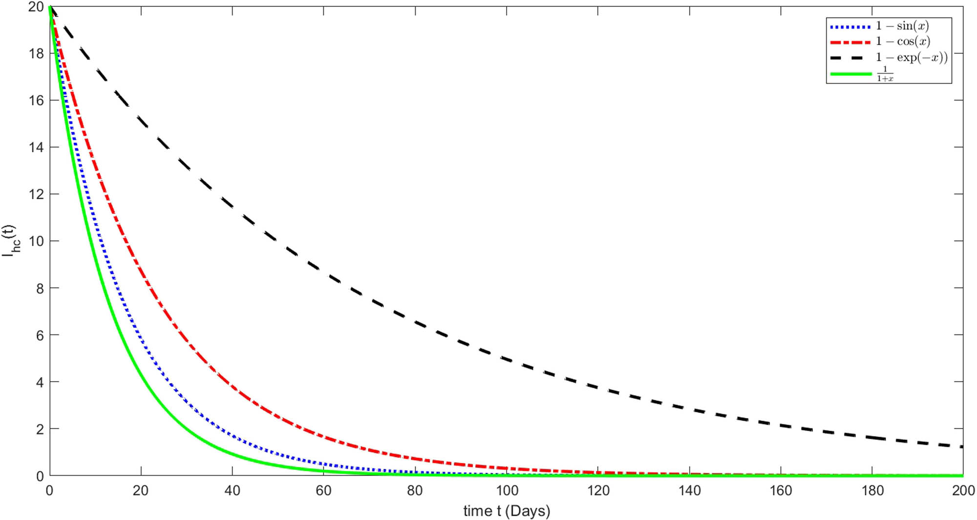
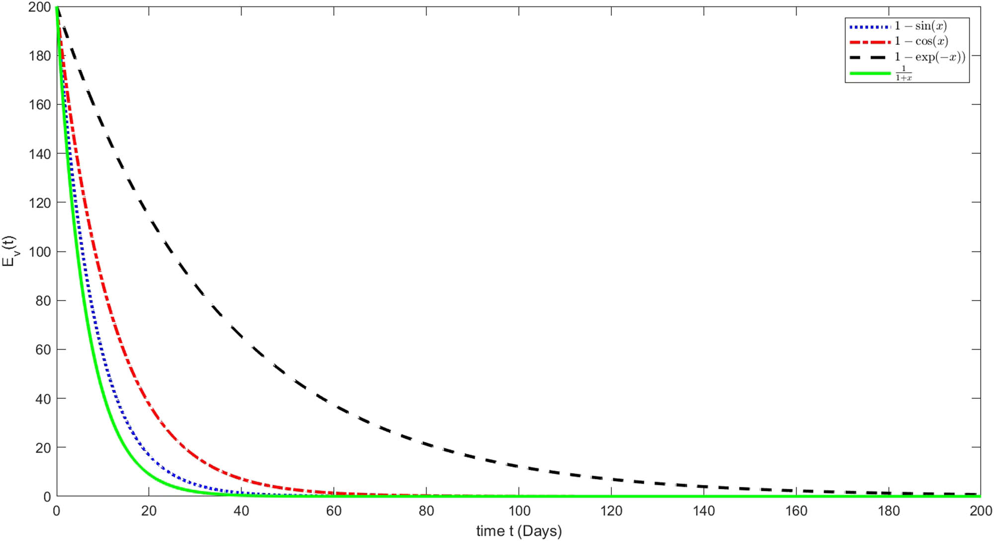
Now, to solve the fractional variable-order LF model numerically, we use the parameter values and initial conditions given in [18], which are as follows:

S h = 1,000 , E h = 100 , I h a = 50 , I h c = 20 , S v = 1,200 , E v = 200 , I v = 300 , Φ h = 0.005802 , μ v = − 0.0008157 , k = 0.000695 , μ h = − 0.2026 , β = 0.0008122 , n = 0.001189 , α h = 0.0007031 , α v = 0.005487 , Φ v = 0.005585 , Ψ = 0.002413 , and ϑ = − 0.1646 . Keeping the mentioned values in the numerical scheme established in (38), we simulate our results graphically in the following Figures 1, 2, 3, 4, 5, 6, 7.

$Figure 1 Graphical presentation of approximate solution of S h {S}_{h} using different variable-orders.$

Figure 1

Graphical presentation of approximate solution of S h using different variable-orders.

$Figure 2 Graphical presentation of approximate solution of E h {E}_{h} using different variable-orders.$

Figure 2

Graphical presentation of approximate solution of E h using different variable-orders.

$Figure 3 Graphical presentation of approximate solution of I h c {I}_{hc} using different variable-orders.$

Figure 3

Graphical presentation of approximate solution of I h c using different variable-orders.

$Figure 4 Graphical presentation of approximate solution of I h a {I}_{ha} using different variable-orders.$

Figure 4

Graphical presentation of approximate solution of I h a using different variable-orders.

$Figure 5 Graphical presentation of approximate solution of E v {E}_{v} using different variable-orders.$

Figure 5

Graphical presentation of approximate solution of E v using different variable-orders.

$Figure 6 Graphical presentation of approximate solution of I v {I}_{v} using different variable-orders.$

Figure 6

Graphical presentation of approximate solution of I v using different variable-orders.

$Figure 7 Graphical presentation of approximate solution of S v {S}_{v} using different variable-orders.$

Figure 7

Graphical presentation of approximate solution of S v using different variable-orders.

We have presented the approximate solutions for different compartments of the proposed model graphically using various values of fractional-order ϖ ( x ) in Figures 1–7. Furthermore, an extension of the Euler method was implemented to establish a numerical scheme aimed at visually presenting the various classes within the model under consideration. Graphical representations of the numerical solution were provided by exploring four distinct variable-order values, specifically ϖ ( x ) = 1 − sin ( x ) , 1 − cos ( x ) , 1 − exp ( − x ) , 1 1 + x , x ∈ [ 0 , T ] in Figures 1–7, respectively. The graphical presentation makes it evident that there is a dynamic decay in susceptible exposed classes, accompanied by noticeable growth in the compartments S h , E h , I h c , I h a , S v , I v , and E v .

5 Conclusion

As earlier, the subject of variable-order fractional calculus deals with differential and integral operators with variable-orders. The concerned derivatives and integrals play significant role in describing various viscoelastic properties more comprehensively as compared to constant fractional-order derivatives. On the other hand, the ABC derivatives with variable-order provide a wide range of applications, because mentioned operators have nonsingular and nonlocal nature and many process with crossover behaviors can be explained very well. Therefore, we have applied fixed point theory to establish the qualitative aspects regarding the existence and uniqueness of solutions for a variable-order dynamical model of LF. In the stability analysis of the LF model (14), Ulam–Hyers stability was deduced by using tools of nonlinear functional analysis. Moreover, a numerical scheme was deduced by using Euler’s method for the considered model. Upon the applications of our numerical scheme, we presented the results graphically using various continuous functions for variable-order. The respective dynamics of various compartments has been interpreted, and the decay and growth phenomenon of various compartments has been shown graphically. In the future, the variable-order ABC, and other differential operators will be applied to investigate other infectious diseases model and chemical evolution process.

Acknowledgments

This work was supported and funded by the Deanship of Scientific Research at Imam Mohammad Ibn Saud Islamic University (IMSIU) (grant number IMSIU-RG23124).

Funding information: This work was supported and funded by the Deanship of Scientific Research at Imam Mohammad Ibn Saud Islamic University (IMSIU) (grant number IMSIU-RG23124).
Author contributions: All authors have accepted responsibility for the entire content of this manuscript and approved its submission.
Conflict of interest: The authors state no conflict of interest.
Data availability statement: All data generated or analysed during this study are included in this published article.

References

[1] Munkhammar J. Riemann-Liouville fractional derivatives and the Taylor-Riemann series. vol. 2004; 2004. p. 1–18. Search in Google Scholar

[2] Atangana A. Mathematical model of survival of fractional calculus, critics and their impact: How singular is our world?. Adv Differ Equ. 2021;2021(1):1–59. 10.1186/s13662-021-03494-7Search in Google Scholar

[3] Shah K, Abdalla B, Abdeljawad T, Alqudah MA. A fractal-fractional order model to study multiple sclerosis: a chronic disease. Fractals. 2024;32(8):2440010. 10.1142/S0218348X24400103Search in Google Scholar

[4] Caputo M. Linear models of dissipation whose Q is almost frequency independent-II. Geophys J Int. 1967;13(5):529–39. 10.1111/j.1365-246X.1967.tb02303.xSearch in Google Scholar

[5] Al-Refai M, Pal K. New aspects of Caputo-Fabrizio fractional derivative. Progr Fract Differ Appl. 2019;5:157–66. 10.18576/pfda/050206Search in Google Scholar

[6] Ghanbari B, Atangana A. A new application of fractional Atangana-Baleanu derivatives: designing ABC-fractional masks in image processing. Phys A Stat Mechanics Appl. 2020;542:123516. 10.1016/j.physa.2019.123516Search in Google Scholar

[7] Zölzer U, Amatriain X, Arfib D, Bonada J, De Poli G, Dutilleux P, et al. DAFX-Digital audio effects. New York: John Wiley & Sons; 2002. Search in Google Scholar

[8] Stone CM, Lindsay SW, Chitnis N. How effective is integrated vector management against malaria and lymphatic filariasis where the diseases are transmitted by the same vector?. PLoS Neglected Tropical Diseases. 2014;8(12):e3393. 10.1371/journal.pntd.0003393Search in Google Scholar PubMed PubMed Central

[9] Ottesen EA, Duke BO, Karam M, Behbehani K. Strategies and tools for the control/elimination of lymphatic filariasis. Bulletin World Health Organization. 1997;75(6):491. Search in Google Scholar

[10] Weerasinghe CR, De Silva NR, Michael E. Maternal filarial-infection status and its consequences on pregnancy and the newborn, in ragama, Srilanka. Ann Tropical Med Parasitol. 2005;99(8):813–6. 10.1179/136485905X65198Search in Google Scholar PubMed

[11] Erickson SM, Thomsen EK, Keven JB, Vincent N, Koimbu G, Siba PM, et al. Mosquito-parasite interactions can shape filariasis transmission dynamics and impact elimination programs. PLoS Neglected Tropical Diseases. 2013;7(9):e2433. 10.1371/journal.pntd.0002433Search in Google Scholar PubMed PubMed Central

[12] Lindsay SW, Denham DA. The ability oi Aedes aegypti mosquitoes to survive and transmit infective larvae of Brugia pahangi over successive blood meals. J Helminthol. 1986;60(3):159–68. 10.1017/S0022149X00026031Search in Google Scholar

[13] Pichon G. Limitation and facilitation in the vectors and other aspects of the dynamics of fi filarial transmission: the need for vector control against Anopheles-transmitted fi filariasis. Ann Tropical Medicine Parasitol. 2002;96(2):S143–52. 10.1179/000349802125002509Search in Google Scholar PubMed

[14] Thirthar AA. A mathematical modeling of a plant-herbivore community with additional effects of food on the environment. Iraqi J Sci. 2023:3551–66. 10.24996/ijs.2023.64.7.34Search in Google Scholar

[15] Thirthar AA, Abboubakar H, Khan A, Abdeljawad T. Mathematical modeling of the COVID-19 epidemic with fear impact. AIMS Math. 2023;8(3):6447–65. 10.3934/math.2023326Search in Google Scholar

[16] Thirthar AA, Naji RK, Bozkurt F, Yousef A. Modeling and analysis of an SI1I2R epidemic model with nonlinear incidence and general recovery functions of I1. Chaos Solitons Fractals. 2021;145:110746. 10.1016/j.chaos.2021.110746Search in Google Scholar

[17] Yousef A, Thirthar AA, Alaoui AL, Panja P, Abdeljawad T. The hunting cooperation of a predator under two prey’s competition and fear-effect in the prey-predator fractional-order model. AIMS Math. 2022;7(4):5463–79. 10.3934/math.2022303Search in Google Scholar

[18] Alshehri A, Shah Z, Jan R. Mathematical study of the dynamics of lymphatic filariasis infection via fractional-calculus. Europ Phys J Plus. 2023;138(3):1–5. 10.1140/epjp/s13360-023-03881-xSearch in Google Scholar PubMed PubMed Central

[19] Coronel-Escamilla A, Gómez-Aguilar JF, Torres L, Escobar-Jiménez RF. A numerical solution for a variable-order reaction–diffusion model by using fractional derivatives with non-local and non-singular kernel. Phys A Stat Mechanics Appl. 2018;491:406–24. 10.1016/j.physa.2017.09.014Search in Google Scholar

[20] Khader MM, Al-Dayel I. Highly accurate technique for studying some chaotic models described by ABC-fractional differential equations of variable-order. Int J Modern Phys C. 2021;32(02):2150018. 10.1142/S0129183121500182Search in Google Scholar

[21] Saxena H. On literature and tools in fractional calculus and applications to mathematical modeling. Int Res. 2021;3(12):1014–9. Search in Google Scholar

[22] Shabani A, Refahi Sheikhani AH, Aminikhah H. Robust control for variable-order time fractional butterfly-shaped chaotic attractor system. J Appl Res Industr Eng. 2020;7(4):435–49. Search in Google Scholar

[23] Abdeljawad T. Fractional operators with generalized Mittag–Leffler kernels and their iterated differintegrals. Chaos Interdisciplinary J Nonlinear Sci. 2019;29(2):023102. 10.1063/1.5085726Search in Google Scholar PubMed

[24] Krasnoselskii MA. Some problems of nonlinear analysis. Amer Math Soc Transl. 1958;10(2):345–409. 10.1090/trans2/010/13Search in Google Scholar

[25] Shah K, Shah L, Ahmad S, Rassias JM, Li Y. Monotone iterative techniques together with Hyers–Ulam-Rassias stability. Math Methods Appl Sci. 2021;44(10):8197–214. 10.1002/mma.5825Search in Google Scholar

[26] Zine H, Lotfi EM, Torres DF, Yousfi N. Tayloras formula for generalized weighted fractional derivatives with nonsingular kernels. Axioms. 2022;11(5):231. 10.3390/axioms11050231Search in Google Scholar

Received: 2023-11-30

Revised: 2024-01-12

Accepted: 2024-02-24

Published Online: 2024-03-20

This work is licensed under the Creative Commons Attribution 4.0 International License.

Articles in the same Issue

https://doi.org/10.1515/phys-2023-0206

Keywords for this article

variable-order differentiation; disease dynamical model; numerical results; existence theory

Creative Commons

BY 4.0